Are Trait–Outcome Associations Caused by Scales Or Particular Items? Example Analysis of Personality Facets and Bmi

Abstract

In personality research, trait–outcome associations are often studied by correlating scale sum scores with an outcome. For example, an association between the NEO Impulsiveness scale and body mass index (BMI) is often interpreted to pertain to underlying trait Impulsiveness. We propose that this expectation can be corroborated by testing for Spearman's theorem of indifference of indicator. Namely, an underlying trait–outcome association should not depend on the specific items (i.e. indicators) used to measure the trait. To test this theorem, we outline an indicator exclusion procedure and demonstrate its viability using a simulation design. We then apply this procedure to test personality–BMI associations for indifference of indicator in a large population–based sample of adult Estonians (N = 2581) using self–ratings and informant ratings obtained with the NEO Personality Inventory–3. Our results show that the N5: Impulsiveness–BMI association mostly depends on two eating–related items, suggesting that the trait associated with BMI may be narrower than the trait the N5: Impulsiveness scale is supposed to measure. Associations between BMI, E3: Assertiveness and C2: Order seem to pertain to the trait. In sum, testing for indifference of indicator provides a potentially useful method to clarify trait–outcome relationships. R scripts are provided that implement the indicator exclusion procedure. Copyright © 2015 European Association of Personality Psychology

Keywords

indifference of indicator Spearman reflective Impulsiveness single item sum score

Introduction

A common method to understand human behaviour is relating various outcomes of interest to personality traits (Ozer & Benet–Martínez, 2006; Roberts, Kuncel, Shiner, Caspi, & Goldberg, 2007). In such analyses, a trait is often operationalised as sum scores of a personality scale consisting of individual items. These individual items of a scale have been chosen to best represent and quantify an ostensibly underlying latent trait—the true personality attribute. Correlations of the scale sum scores with outcomes of interest are then interpreted as pertaining to the underlying trait. However, we argue that such interpretations may sometimes merit more careful consideration, particularly if traits are indeed conceptualised as latent variables.

In latent variable framework, the true variance of a personality trait is manifested in the common variance of scale's items (further described later). If so, to the extent that a correlation between a scale's sum score and an outcome reflects the correlation of the outcome with an underlying trait, the association should be independent of how the underlying trait is measured. In particular, the association should not depend on which items happen to be sampled for the measurement of the trait. Otherwise, the association would not pertain to the underlying trait, but to the specific characteristics reflected in the particular items driving the observed correlation. This may sound like a trivial assumption, but it is often neglected in practice.

For example, the N5: Impulsiveness facet of the NEO Personality Inventory (NEO–PI–R) has been related to body mass index (BMI) in several studies (Sutin, Costa et al., 2013; Sutin, Ferrucci, Zonderman, & Terracciano, 2011; Sutin et al., 2015; Terracciano et al., 2009). However, not all N5: Impulsiveness items relate to BMI. Terracciano et al. (2009) specify that

the Impulsiveness scale effect [on BMI] was due to two items specific to the eating domain (‘When I am having my favorite food, I tend to eat too much’ and ‘I sometimes eat myself sick’) (p. 685).

Although this may seem to provide little evidence for trait Impulsiveness being associated with BMI, follow–up studies have still concluded that Impulsiveness relates to BMI without testing the crucial role of the two aforementioned items behind this association (Sutin, Costa, et al., 2013; Sutin et al., 2011, 2015; see Iacovino, Powers, & Oltmanns, 2014, for a notable exception).

It should be noted that the same logic has already been applied in the context of the Big Five domains and their facets. In particular, there is ample evidence that different facets of the same Big Five domain scales correlate with outcomes in different ways (e.g. Costa & McCrae, 1995; Judge, Rodell, Klinger, Simon, & Crawford, 2013). Therefore, facets reflecting the same trait should relate to outcomes in similar ways if the associations pertain to the underlying domain–level trait. If they do not, then the associations pertain to facet(s) and not to the domain–level trait. This logic is commonly accepted as can be seen in Sutin et al. (2011): Although they demonstrate that BMI relates to trait Neuroticism, they appropriately interpret the effect being driven by the N5: Impulsiveness facet. We propose that the same logic should be extended to indicators of single traits or facets, that is, to single items.

There is increasing evidence that the personality trait hierarchy may be meaningfully extended below facets. A recent analysis of cross–rater agreement across broad domains, facets, and single items concluded that there was a significant amount of descriptive variance left in NEO–PI–3 items that raters agreed on, once the effects of broad domains and facets had been removed (Mõttus, McCrae, Allik, & Realo, 2014). Similarly, another paper attempted to build unidimensional confirmatory factor analysis models of NEO–PI–3 facets; to achieve reasonable fit indices, almost all facets required allow additional residual correlations between items (S2 in Mõttus et al., 2015), demonstrating additional covariance—and thereby ‘signal’—below the facets. McCrae (2014) suggested that trait–like characteristics below the level of facets should be called nuances. As these nuances have not been documented yet, we reserve our analysis to items. Similar to nuances, single items might reflect different small trait–like features.

The benefit of understanding what causes a scale–outcome association is schematically shown in Figure 1. When there is a domain–level association with an outcome, then all the sub–indicators should be correlated with the outcome as well (Figure 1A). When the association pertains to the facet instead of the domain (Figure 1B), then there might be a weaker domain–level correlation. However, it is more precise to claim that the facet is causing the trait–outcome association, not the broad domain. Similarly, if there is a strong true association between single item (or nuance) and an outcome, a diluted effect might be visible at facet or even at domain level. However, it would be more precise to attribute the association to the nuance.

Figure 1

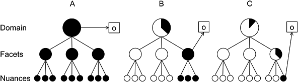
Trait–outcome associations at different levels of personality measurement. Filled circle = trait's association with an outcome that is indicator indifferent. Semi–filled circle = trait's association with an outcome that depends on a certain indicator. Empty circle = no association between trait and outcome. (A) Outcome relates to the domain–level trait. Therefore, the outcome also relates to all domain's indicators (i.e. facets), and also to all indicators of facets (i.e. items, also interpretable as nuances (McCrae, 2014)). (B) Outcome relates to the facet–level trait. The outcome could also correlate with the domain–level trait sum score. However, because the outcome only correlates with a single indicator of the domain, the outcome pertains only to the facet level as such. (C) Outcome relates to a single nuance. The association might be visible also at domain– and facet–level sum scores. However, in both cases, no other indicators relate to the outcome. Therefore, the association pertains to the nuance level.

Indifference of indicator: Theoretical background

The logic outlined earlier originates from Spearman's (1927) theorem called indifference of indicator (ION¹). He introduced ION in the context of measuring general intelligence (g):

for the purpose of indicating the amount of g possessed by a person, any test will do just as well as any other, provided only that its correlation with g is equally high (Spearman, 1927, p. 197).

In intelligence research, this theorem has enjoyed notable popularity (reviewed in Horn & McArdle, 2007) and has received strong empirical support (Johnson, Bouchard, Krueger, McGue, & Gottesman, 2004; Johnson, te Nijenhuis, & Bouchard, 2008). We propose that it could equally be applied in personality research. In particular, we articulate some conditions that must be fulfilled for a trait–outcome association to be indifferent of its indicators. We also propose a statistical procedure that tests whether a trait–outcome association is indicator indifferent. We discuss ION in the context of single items being indicators for a particular trait, but the same logic also applies, in principle, when facets are considered indicators of a broader latent domain.

Here, we take the assumption that personality traits are of reflective type, whereby the trait is a latent common cause of its indicators (e.g. items; Bollen & Lennox, 1991; Borsboom, Mellenbergh, & van Heerden, 2003). Although we acknowledge that there may be other views as to the nature of personality traits and embrace them, assuming traits to be reflective seems to be the most common trait interpretation (Borsboom, 2006; DeYoung, 2014; McCrae, 2014). According to this interpretation, the true variance of a trait is manifested in the common variance of its indicators. The common variance can be explicitly modelled, as in case of latent trait modelling, or assumed to emerge via aggregation, as in case of classical test theory applications. The indicators are ‘noisy’, and the degree to which they reflect the underlying latent trait can be expressed in terms of factor loadings or item–total correlations.

Consequently, if an outcome correlates with a trait, none of the trait's indicators (i.e. items) should correlate with the outcome more than the aggregate trait score. This is because the associations between single indicators and the outcome are indirect, mediated by the underlying trait. Single indicator–outcome correlations should then equal the products of the trait–outcome correlation and the factor loadings of the respective indicators. Therefore, the single indicator–outcome correlations should be proportional to their factor loadings, if it is only the latent trait that correlates with the outcome. However, this might not always be the case, as seen in the N5: Impulsiveness–BMI association addressed earlier. It seems that personality scales have not always been explicitly designed to be unidimensional (cf. Gerbing & Anderson, 1988; Gorsuch, 1997). Therefore, the items in a scale might have other sources of covariance than the trait they have been intended to measure. When such a scale is related to the outcome, it might not be the main trait but these other sources of covariance that cause the correlation between a scale and an outcome. In the case of N5: Impulsiveness, it seems that only eating–related items and not generic impulsivity items are associated with BMI. The question then is this: How can we test if an outcome relates to the trait itself or only to a certain subset of its indicators?

Methods for detecting indifference of indicator

A natural test of ION would be to measure a purported trait with multiple scales that sample different indicators of the trait and have roughly similar reliabilities or determinacies: If ION holds, their correlations with the outcome should be similar (Mõttus, Luciano, Starr, Pollard, & Deary, 2013). However, researchers can rarely afford to measure traits with multiple scales.

One may then estimate the presence of ION by correlating the outcome of interest to single items. This is a very straightforward procedure but appears rarely employed in practice. If most items of a scale correlate with the outcome and the correlations are in the same direction, this may be consistent with the presence of ION; preferably, no single item–outcome correlation should exceed the scale–outcome correlation, as was discussed earlier. However, this method does not provide a formal test for deciding, whether some items violate the principle of ION. For example, some variability across items in their outcome correlations is expected owing to differential factor loadings or measurement noise.

To obtain a more formal test of ION, one could employ the ‘method of correlated vectors’ (Jensen, 1998). According to this method, there should be a positive correlation between the factor loadings and outcome correlations of trait indicators. Indicators deviating from the regression line can be considered to violate ION. However, this method has been criticised on several grounds. For example, it appears to be severely biased in favour of observed associations pertaining to the underlying trait (Lubke, Dolan, & Kelderman, 2001) and also sensitive to the selection of trait indicators (Ashton & Lee, 2005).

Therefore, a procedure devoted to testing ION is needed. We propose a simple indicator exclusion approach that provides an opportunity to statistically test whether a scale–outcome relationship meets the ION assumption and, if it does not, which items are causing the lack of ION. Namely, stemming from the principles of ION, it should not matter which items happen to be used to capture the trait. Therefore, one can systematically exclude any single item from a scale and observe the resulting changes in trait–outcome correlations. The correlations between original trait–outcome and reduced–trait outcome trait should not differ much from each other if it is the underlying trait that is related to the outcome. However, these correlations are likely to vary more if only certain items of a scale relate to the outcome. For instance, in the example of N5: Impulsiveness, if it is trait Impulsiveness that relates to BMI, the scale–outcome correlation should not change much, when the eating–related items are removed from the scale. However, if such removal causes the scale–outcome correlation to change or vanish altogether, this implies that the scale's association with BMI is to some extent or entirely specific to certain items.

The detailed procedure is as follows. For each item, correlation between the scale's sum scores and outcome is calculated such that the particular item is excluded from the sum scores.² Each of the obtained correlations will then be compared with the original scale–outcome correlation (sum score of all items). This comparison can be conducted with William's test for two dependent correlations that share one variable (Steiger, 1980). William's test characterises difference between correlations with a p–value—a small p–value indicates that the tested difference between correlations is unlikely to have happened by chance and could be considered a real difference. Thus, each item will receive a p–value characterising the ‘significance’ of difference between correlations—here called ‘significance of indicator exclusion’ (SONE²).

The items are then ordered according to the SONE. If the lowest SONE is above a certain p–criterion (defined later), the trait–outcome relationship can be considered indicator indifferent. Conversely, if there is an item with a SONE below a conventional criterion, partial or complete lack of ION is likely due to that particular item. Therefore, the item with the lowest SONE should be excluded from the scale to establish an indicator–indifferent trait–outcome relationship. The whole procedure is then repeated on the remaining set of items to determine if any additional items are compromising ION. The procedure stops if no more items obtain a SONE below the criterion. As a result, the list of excluded items represents items that have a correlation with the outcome independent of the scale's ostensible underlying trait.

As always, there is a question of an optimal criterion p–value. The significance criterion has to be a trade–off between Type I and Type II errors, given sample size. In smaller samples, the power to detect correlation difference is smaller, and therefore, a more lenient criterion is needed (which obviously increases Type I error rate). In large samples, the procedure is likely to flag very small changes in correlation as significant, even if it does signal only trivial lack of ION. To establish an optimal significance criterion for a given sample size, a simulation was conducted. The simulation modelled scale–outcome associations that either had or did not have ION. An optimal cut–off criterion was selected that minimised the likelihood of excluding items if the association was indicator indifferent and maximised the likelihood of excluding items if the association was lacking ION.

Aims of the paper

The current paper seeks to outline the method and the usefulness of testing trait–outcome associations for ION. Study 1 used simulations to demonstrate and test the viability of the proposed indicator exclusion method and establish appropriate p–value criteria. In Study 2, the procedure was applied to empirical data by means of replicating BMI–personality trait associations (Terracciano et al., 2009) in a large population–based sample of adult Estonians. Scales that were significantly correlated with BMI were tested for ION. The BMI–personality relationship was chosen as some papers have explicitly tested if Impulsiveness–BMI association depends on a few items (Iacovino et al., 2014; Terracciano et al., 2009) of the N5: Impulsiveness scale, whereas other papers have not (Sutin, Costa, et al., 2013; Sutin et al., 2011, 2015). The BMI–personality dataset includes both self–reports and informant reports. Given that informant ratings are considered as reliable as self–ratings of personality (Kolar, Funder, & Colvin, 1996), we assume that any robust association will replicate across both rating types. This could be taken as a case of constructive replication (Lykken, 1968).

Study 1: Simulation Study

The goal of the simulation study was to show that ION could be tested with the indicator exclusion approach. The procedure was tested on simulated scales and outcomes, whose relations were or were not indifferent of indicator. We expected that the procedure would correctly highlight items that caused lack of ION between scales and outcomes. The secondary goal of the simulation study was to provide relevant significance criteria for Study 2.

Simulation methods

A trait scale and outcome were simulated according to two sets of scenarios (Figure 2). First, consistent with ION, scores of a single normally distributed trait (t) were simulated (N = 1000, μ = 0, σ = 1). This trait was allowed to contribute to an outcome (o) with a standardised regression weight β, such that o = β * t + ε_t, where ε_t was a normally distributed random error term (μ = 0, σ = 1). We tested three different β values 0.15, 0.25 and 0.35. Main focus is on β = 0.25 as such seems to be the effect size of trait N5: Impulsiveness–BMI association in Study 2. The simulated trait was manifested in a scale consisting of eight items. The items had factor loadings λ ranging from 0.4 to 0.7; arguably, these may be seen as rather desirable parameter values (e.g. Ford, MacCallum, & Tait, 1986). We chose to have eight items per scale, similar to the NEO–PI scales, so that the results of Study 1 could be applied in Study 2. This scale is referred to as ‘8 + 0’, indicating that scale does not have any items referring to a secondary trait.

Figure 2

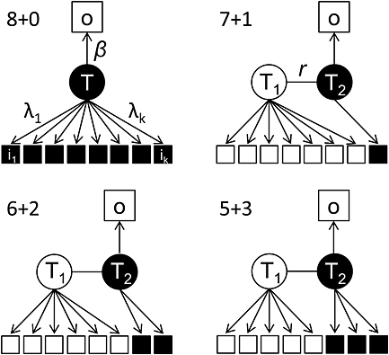
Diagrams of the different scales modelled. In 8 + 0 scenario, the scale–outcome association is indicator indifferent. In other scenarios, the scale–outcome association pertains to a subset of items reflecting a separate trait (T₂). Rectangles are observed items or outcomes, and circles denote latent variables. Shapes filled with black denote outcome–related traits and indicators, and white shapes are not related to an outcome. Model parameters are shown once, although they apply in several scenarios. β = trait–outcome association; λ = factor loading; i = item; k = number of items in a scale, here k = 8; o = outcome; r = correlation between traits; T = trait; T₁ = trait not related to outcome; T₂ = trait related to outcome.

A second set of scenarios reflected lack of ION owing to the lack of unidimensionality in the scale. Instead of a single underlying trait, a composite scale consisting of two underlying correlated traits (T₁ and T₂) was created. Here, T₁ represented the main trait that the scale was purported to measure, whereas T₂ represented a trait related to but distinct from T₁. Crucially, only T₂ was allowed to contribute to the outcome o, which mimics the situation where only a subset of a scale drives the correlation with an outcome. We tested three association strengths: β = 0.15, 0.25 or 0.35. Otherwise, the same procedure as earlier was followed. The correlation between T₁ and T₂ was set at 0.3, reflecting rather typical inter–facet correlation of personality questionnaires (Ostendorf & Angleitner, 1994). Three versions of an eight–item scale lacking ION were simulated, in which seven to five items were manifestations of T₁, and, respectively, three to one items were manifestations of T₂. Otherwise, the same item generation procedure as earlier was used. These three scales lacking ION are referred to as ‘7 + 1’, ‘6 + 2’ and ‘5 + 3’.

All scenarios were simulated 10 000 times. Within a simulation, scale–outcome associations were analysed with the indicator exclusion procedure. In scale with ION (8 + 0), no item was excluded. However, we did record the lowest SONE value that was necessary for obtaining an optimal p–value (see succeeding texts).

A similar procedure was conducted with scales without ION (7 + 1, 6 + 2, 5 + 3). Besides calculating the lowest SONE value, we also designed the procedure to remove the item with the lowest SONE and then repeat itself, until no items were supposedly left in T₂. For instance, in the case of 7 + 1, we first calculated the lowest SONE, then excluded the respective item and calculated the lowest SONE again based on seven items (referred to as ‘7 + 0’). To estimate the accuracy of the procedure, we inspected whether the item excluded did in fact belong to T₂. A similar procedure was conducted on 6 + 2, where one item was excluded first (6 + 1) and another excluded thereafter, leaving a scenario where no more items should be removed (6 + 0).

As stated in the section on Methods for Detecting Indifference of Indicator, the optimal p–criterion should be low enough to minimise the likelihood of excluding items when ION in fact exists. Therefore, p–criterion has to be lower than the lowest SONE value in a scenario where no items should be removed from the scale (8 + 0, 7 + 0, 6 + 0, 5 + 0). At the same time, the criterion should be high enough to maximise the likelihood of excluding items if the association is lacking ION. Therefore, the p–criterion has to be higher than the lowest SONE value in scenarios lacking ION (7 + 1, 6 + 2 and 5 + 3, and also 6 + 1, 5 + 2 and 5 + 1).

For all SONE mean values, we also depicted 95% confidence intervals. All simulations were conducted on sample sizes 100, 250, 500, 750, 1000, 2500 and 5000 and with three different β values. Analyses were conducted in R environment (R Core Team, 2013), occasionally relying on ‘psych’ package (Revelle, 2014).

Results and Discussion

Table 1 shows how the item exclusion's accuracy depends on both the effect size in question and sample size. For larger effects (β = 0.35), violations of ION can be reasonably accurately (95%) detected in samples of 500 or more, whereas for β = 0.15, one would need a sample size of 2500 or more to achieve a comparable level of accuracy. Although the item exclusion procedure requires relatively large samples if expected effect sizes are small, it may be a promising method to detect items causing lack of ION.

Table 1

Percent of correctly excluded items across scenarios lacking ION

β	Scenario	Sample size
β	Scenario	100	250	500	750	1000	2500	5000
0.35	7 + 1	46.02	76.15	93.74	98.31	99.42	100	100
	6 + 2	61.08	86.15	97.12	99.41	99.89	100	100
	6 + 1	38.65	67.82	90.19	97.28	99.17	100	100
	5 + 3	67.83	86.82	96.31	99	99.75	100	100
	5 + 2	56.79	81.46	95.86	98.96	99.77	100	100
	5 + 1	37.13	62.82	87.84	96.08	98.74	99.98	100
0.25	7 + 1	30.65	53.44	77.8	89.09	94.67	99.94	100
	6 + 2	46.18	68.96	87.39	95.02	97.91	99.97	100
	6 + 1	28.69	47.29	70.38	84.29	91.89	99.84	100
	5 + 3	55.4	73.61	88.42	94.02	97.06	99.89	100
	5 + 2	44.81	64.58	82.92	92.5	96.08	99.96	100
	5 + 1	27.56	44	66.18	80.84	89.66	99.66	100
0.15	7 + 1	19.68	31.3	45.89	57.61	67.77	93.43	99.35
	6 + 2	32.72	45.23	61.05	72.94	80.25	97.21	99.87
	6 + 1	19.2	27.45	39.6	50.04	60.06	90.5	99
	5 + 3	44.71	54.22	67.7	75.68	81.75	96.6	99.65
	5 + 2	34.3	42.8	57.29	66.82	74.54	95.65	99.69
	5 + 1	20.37	26.21	36.82	47.4	56.87	87.56	98.61

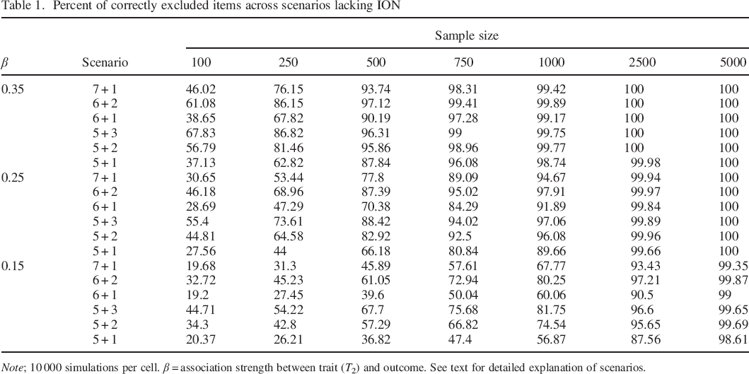
Note; 10 000 simulations per cell. β = association strength between trait (T₂) and outcome. See text for detailed explanation of scenarios.

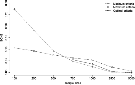
However, in real data, we do not know a priori how many items need to be removed. Therefore, p–criteria are needed for one to be able to decide how many and which items to exclude. To define the maximum and minimum criteria, the average SONE values were calculated across simulations for all sample sizes. The results for β = 0.25 are depicted in Figure 3. It can be seen that mean SONE was greater for scales with ION (solid lines in Figure 3B–D) than for scales without ION (dashed lines in Figure 3B–D) for all sample sizes. This suggests that an optimal p–value can be found that lies between those two extremes. Further, once the samples became 1000 or more, the confidence intervals for the scales that lack ION (dashed lines in Figure 3B–D) became smaller, suggesting that lack of ION could be more clearly detected in larger samples. Similar figures β = 0.15 and β = 0.35 can be seen in the Supporting Information (Figures S1 and S2).

Figure 3

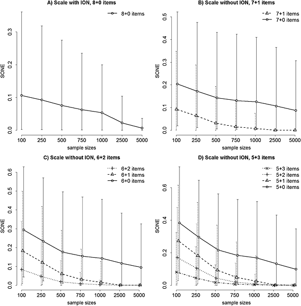
Mean minimum ‘significance of indicator exclusion’ (SONE) values across different simulation conditions and different sample sizes. (A) The scale was designed to have an indicator–indifferent (ION) relationship with an outcome. (B–D) The scale–outcome relationship was not indicator indifferent, such that most items correlated with the main trait (T₁), but the outcome related to a sub–trait (T₂) represented by one to three items only. The T₂–related items were then iteratively removed (e.g. 5 + 2 refers to a scale from which one item had been removed). Trait–outcome association (β) = 0.25.

To define the maximum values of the p–criteria, we first identified the lowest mean SONE across scenarios where no items had to be removed, which in case of β = 0.25 corresponded to the lowest solid line across Figure 3 (i.e. Figure 3A). Thereafter, to define the minimum values for the p–criteria, we identified the highest SONE values when a trait was lacking ION, which corresponded to the highest dashed line across Figure 3 (i.e. 1 + 5 scenario in Figure 3D). These two scenarios have been plotted again in Figure 4.

Figure 4

Detecting optimal p–criteria. Minimum criteria: highest ‘significance of indicator exclusion’ (SONE) values that excluded items causing lack of indifference of indicator (scenario 5 + 1 from Figure 3D). Maximum criteria: lowest SONE values that did not exclude items that belonged to a trait related to outcome (scenario 8 + 0 from Figure 3A). Optimal criteria: geometric mean between minimum and maximum. Trait–outcome association (β) = 0.25.

Apparently, in smaller samples, it was impossible to find an optimal p–value, as minimum criteria were larger than maximum criteria (Figure 4). In case of β = 0.25, 750 was the minimum sample size from which onwards it was possible to obtain p–values (Figure 4). A likely reason is that with smaller sample sizes, it is very hard to reliably exclude the correct item in a 5 + 1 scenario—the uncertainty of this scenario is also illustrated by relatively wide confidence intervals in Figure 3(D) and with lowest percent of correctly excluded items in Table 1 . Where it was possible to find and optimal p–value, this value was determined by the geometric mean between maximum and minimum. Optimal p–values for different effect sizes and scenarios are provided in Table 2. Here is an example with a sample size of 2500 and β = 0.25: If removal of an item causes the scale–outcome correlation to change with a significance below 0.0037, then this item is causing violation in ION and has a separate relationship with the outcome.

Table 2

Optimal p–values for different trait–outcome associations and sample sizes

β	Sample size
β	100	250	500	750	1000	2500	5000
0.35	–	–	0.039	0.018	8.6 * 10⁻³	1.7 * 10⁻⁴	1.2 * 10⁻⁷
0.25	–	–	–	0.055	0.036	3.7 * 10⁻³	9.0 * 10⁻⁵
0.15	–	–	–		–	0.041	9.4 * 10⁻³

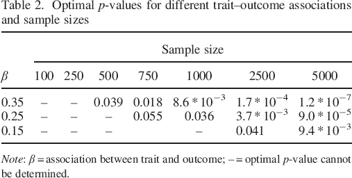
Note: β = association between trait and outcome; – = optimal p–value cannot be determined.

Study 2: Personality–BMI Relationships

Next, we sought to apply the tools outlined in the simulation analysis to study the presence or absence of ION in personality scale–BMI associations. We first screened for personality traits that related to BMI in both self–report and informant report. This also enabled us to verify whether ION testing would replicate.

Methods

Participants

Participants were drawn from the Estonian Genome Center, University of Tartu (EGCUT). The EGCUT was launched as an initiative of the Estonian Government in 2001 to create a database of health, genealogical and genome data representing 5% of the Estonian population (Leitsalu et al., 2014). EGCUT participants were randomly selected from individuals visiting general practitioners (GPs) and hospitals, recruited by GPs and hospital physicians. All participants gave informed consent. In addition to donating blood samples and answering a medical questionnaire, participants were asked to complete the self–report version of a comprehensive personality test and find a knowledgeable informant who could complete the same questionnaire about them.

In total, the sample used in the present study included 2581 people (of whom 1398 were women) with a mean age of 44.0 years (SD = 17.3, ranging from 18 to 90 years) and a mean BMI of 26.08 (SD = 4.9, ranging from 15.9 to 54.1). Participants’ weight and height were measured when they were recruited. Percent overweight (BMI > 25) in this sample is 52.9%, which matches a survey–based prevalence estimation of 49%, based on 5000 Estonians (Tekkel & Veideman, 2013). However, another estimate that objectively weighed 495 participants representing the population suggested that prevalence of overweight status might reach 67% (Eglit, Ringmets, & Lember, 2013). Of the 2581 participants, 8.2% people had elementary education, 24.5% had secondary school education, 27.9% had secondary specialised education and 39.4% had a higher education degree. Of the informants, 52% were spouses or partners, 15% friends, 15% parents, 6% children or grandchildren, 6% siblings, 3% acquaintances and 3% other relatives. The informants were 72% female, and the mean age of informants was 42.4 years (SD = 16.1, ranging from 11 to 89 years). Overall, 5.6% of informants had elementary education, 25% had secondary education, 27.1% had secondary specialised education and 42.2% had a higher educational degree.

Measures

The NEO Personality Inventory–3 (NEO–PI–3; McCrae & Costa, 2010) is a slightly modified version of the NEO PI–R questionnaire (Costa & McCrae, 1992) that was translated into Estonian by Kallasmaa and colleagues (Kallasmaa, Allik, Realo, & McCrae, 2000). Like the original NEO PI–R, the NEO–PI–3 has 240 items, which measure 30 personality traits grouped into the five–factor model domains. The NEO–PI–3 has excellent psychometric properties in a wide range of countries, including Estonia (De Fruyt, De Bolle, McCrae, Terracciano, & Costa, 2009). Participants themselves completed the self–report form of the NEO–PI–3. Informants completed the observer report form. In line with typical findings (Connolly, Kavanagh, & Viswesvaran, 2007), the correlations between the respective scale scores based on self–reports and informant reports were 0.53, 0.66, 0.61, 0.47 and 0.53 for Neuroticism, Extraversion, Openness, Agreeableness and Conscientiousness, respectively, and ranged from 0.39 to 0.62 (median = 0.46) for the 30 facet scales. For single items, the self–report–informant report correlations ranged from 0.13 to 0.56 (median = 0.30). All reported correlations were significant at p < 0.01.

Analytic strategy

Body mass index was log–transformed owing to its skewed distribution and residualised for the effects of age, gender and education, as these variables might have confounded personality–obesity relationships (Armon, Melamed, Shirom, Shapira, & Berliner, 2013; Brummett et al., 2006; Ogden et al., 2006; Rolls, Fedoroff, & Guthrie, 1991; Sutin, Costa et al., 2013; Tekkel & Veideman, 2013). First, a correlation analysis of BMI and NEO–PI–3 domain and facet scales was performed as a replication of earlier studies (Sutin et al., 2011; Terracciano et al., 2009). Only scales significantly (p < 0.01) correlating with BMI in both self–reports and informant reports were taken further for the ION testing procedure. For ION testing, the optimal p–criterion was chosen based on the previously described simulation results, considering our sample size and assumed trait–outcome association (β), which was set close to the highest single item–outcome correlation. We preferred single item correlations because if a scale violated ION, and then the sum score–outcome correlation could be misleadingly low (Figure 1). In the indicator exclusion procedure, indicators causing violation in ION were excluded iteratively until no SONE value was below the criteria. The results were plotted in a single item–outcome correlation plot, with excluded items highlighted (Figure 5, ‘single indicator–outcome correlation’). To further demonstrate that the excluded items might have their own relationship with the BMI, the scale–BMI relationship was graphed with and without the excluded items (Figure 5, ‘Scale–outcome correlation’). Some scale–BMI correlations were too small to be properly tested for ION; in these cases, only the single item–outcome correlations were plotted for preliminary assessment of ION (Figure 6). Barplots were plotted using ‘gplots’ package (Warnes et al., 2014).

Figure 5

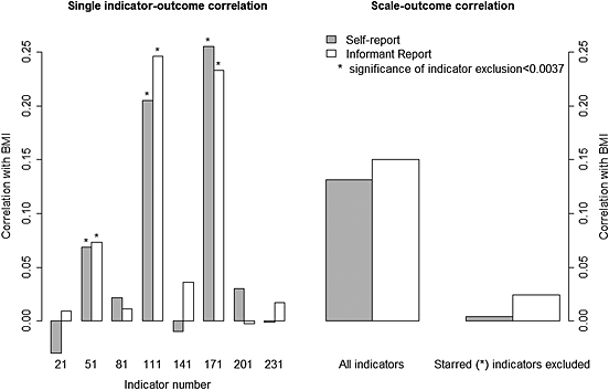
Testing relationship between body mass index (BMI), and N5: Impulsiveness for indifference of the indicator with indicator exclusion procedure.

Figure 6

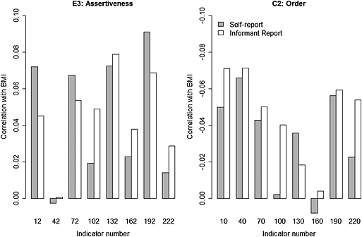
Single item–outcome associations between body mass index (BMI), E3: Assertiveness and C2: Order.

Results

Correlations between BMI and personality scales

Table 3 lists the generally weak correlation coefficients between BMI and personality scales in both self–ratings and informant ratings. Three facets correlated with BMI in both self–report and informant report and were thus selected for further analysis: BMI related positively to N5: Impulsiveness and E3: Assertiveness and negatively to C2: Order.

Table 3

Residualised correlation coefficients between personality traits and BMI, across self–ratings and informant ratings

Domain/facet	Self	Informant
Domain/facet	r _p	r _p
Neuroticism	0.03	0.04
Extraversion	0.04	0.03
Openness	0.00	0.02
Agreeableness	0.00	−0.01
Conscientiousness	−0.04	−0.05
N1: Anxiety	0.01	0.03
N2: Angry Hostility	0.02	−0.01
N3: Depression	0.01	0.03
N4: Self–consciousness	0.03	0.01
N5: Impulsiveness	0.13	0.15
N6: Vulnerability	−0.04	−0.02
E1: Warmth	0.04	0.06
E2: Gregariousness	0.00	0.02
E3: Assertiveness	0.07	0.06
E4: Activity	−0.01	−0.02
E5: Excitement–Seeking	0.00	0.00
E6: Positive Emotions	0.07	0.04
O1: Fantasy	0.04	0.03
O2: Aesthetics	0.01	−0.01
O3: Feelings	0.00	0.03
O4: Actions	−0.02	0.01
O5: Ideas	0.00	−0.01
O6: Values	−0.03	0.01
A1: Trust	−0.02	−0.01
A2: Straightforwardness	−0.03	−0.04
A3: Altruism	0.01	0.02
A4: Compliance	−0.03	0.01
A5: Modesty	0.02	0.00
A6: Tender–mindedness	0.04	−0.02
C1: Competence	0.02	0.00
C2: Order	−0.06	−0.07
C3: Dutifulness	−0.03	−0.02
C4: Achievement Striving	−0.04	−0.05
C5: Self–Discipline	−0.02	−0.06
C6: Deliberation	−0.02	−0.01

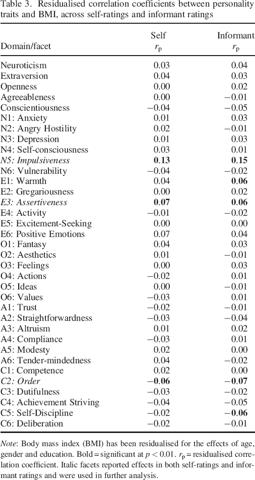
Note: Body mass index (BMI) has been residualised for the effects of age, gender and education. Bold = significant at p < 0.01. r_p = residualised correlation coefficient. Italic facets reported effects in both self–ratings and informant ratings and were used in further analysis.

Testing scale–BMI associations for ION

The optimal p–criterion for N5: Impulsiveness was 0.0037, as some items approached a correlation of 0.25 with BMI (Table 2, Figure 5). The N5: Impulsiveness failed to meet ION (Figure 5). In particular, indicator exclusion procedure suggested that scale's relationship with BMI depended on two eating–related items⁴ (#111—‘I tend to eat too much of my favourite food’ and #171—‘Sometimes I am not able to control my appetite’), as well as a more general impulse control item (#51—‘It is hard for me to control my impulses’).

The effects of other scales were too small for properly testing for ION. Simulations with β = 0.10 and n = 2500 had revealed that percentage of correctly excluded items could range from 60% to 85% and that optimal p–criterion could not be determined. However, for a preliminary assessment, we plotted the single item–outcome correlations. Figure 6 suggests that, in contrast to N5: Impulsiveness, the associations of E3: Assertiveness and C2: Order scores with BMI were more likely to pertain to the core traits of the scales as over half of the items related to the outcome in a roughly equal level. At the same time, there were small inconsistencies as some items had very low correlation—future studies with higher power can formally test these associations for ION.

Discussion

Testing personality–BMI relationships revealed that the well–documented correlation between BMI and Impulsiveness depended on a subset of items, mostly those relating to eating. The associations therefore fail to meet the assumption of ION. The effects of E3: Assertiveness and C2: Order were more likely to be indicator indifferent, but we were unable to formally test these associations owing to small effect sizes. All these effects manifested in both self–reports and informant reports, supporting the robustness of the findings.

There could be two explanations for the lack of ION in case of N5: Impulsiveness–BMI association. First, the two eating–related items could reflect eating–related impulsivity, a construct that has been suggested to be more BMI relevant than domain–general impulse control across various measures (Houben, Nederkoorn, & Jansen, 2013; Rasmussen, Lawyer, & Reilly, 2010; Tsukayama, Duckworth, & Kim, 2012; also Vainik, Dagher, Dubé, & Fellows, 2013). For instance, the three BMI–related items from Impulsiveness relate strongly to other eating–related scales (Vainik, Neseliler, Konstabel, Fellows, & Dagher, 2015). Another interpretation could be that items asking about overeating are logically so close to BMI as to make any meaningful conclusion difficult. Namely, people might observe first that they are overweight and then conclude that they are unable to control themselves. For instance, N5: Impulsiveness is known to change in parallel with weight status (Sutin, Costa et al., 2013). Whichever stance is taken, either of these interpretations is more precise than claiming that trait Impulsiveness is the underlying attribute relating to BMI. Based on these results, there would be no point saying it is impulsiveness as some sort of underlying trait that correlates with BMI, and this is an important finding in its own right.

The sum score of N5: Impulsiveness has been related to several other interesting outcomes, including BMI change, eating behaviours and disorders, leptin levels, white blood cell counts, drug and alcohol consumption, gambling and brain activity, such as dopamine secretion and reward responsiveness (Bagby et al., 2007; Elfhag & Morey, 2008; Jen, Saunders, Ornstein, Kamali, & McInnis, 2013; Oswald et al., 2007; Ruiz, Pincus, & Dickinson, 2003; Sutin, Costa et al., 2013; Sutin, Evans, & Zonderman, 2013; Sutin, Zonderman et al., 2013; Sutin et al., 2011, 2012; Villafuerte et al., 2012). It would be interesting to reanalyse these effects for ION to understand if these outcomes pertain to trait Impulsiveness as the underlying attribute, or something more specific (cf. Iacovino et al., 2014; Terracciano et al., 2009).

The effects of E3: Assertiveness and C2: Order on BMI are very small, but they have been repeatedly found across several studies (Sutin et al., 2011; Terracciano et al., 2009). The effect of Order suggests that more organised persons have lower risk for obesity. A potential mechanism could be consistency in eating patterns—having similar meals across eating episodes has been shown to relate positively to successful weight maintenance and other health indices (Gorin, Phelan, Wing, & Hill, 2003; Pachucki, 2012; Wing & Phelan, 2005; see Vainik, Dubé, Lu, & Fellows, 2015, for further discussion). The effect of assertiveness seems to be instrument specific; studies with other personality instruments suggest instead that lack of assertiveness relates to maladaptive eating behaviours (Elfhag, 2005; Elfhag & Erlanson–Albertsson, 2006). This, obviously, points to potential lack of ION, which could be tested by linking items from multiple assertiveness scales to BMI scale.

General Discussion

The current paper has outlined a procedure to test if a trait–outcome association pertains to the whole scale or to its particular items. Guided by Spearman's (1927) theorem of ION, we suggest that all indicators of an underlying trait should similarly relate to the outcome. To apply this theorem in a personality context, we designed an indicator exclusion procedure that tests whether exclusion of an item significantly influences scale–outcome correlation.

Testing for ION is likely to be widely applicable, given that most personality trait–outcome research has so far been exclusively based on linking outcomes with aggregate scores. The point we want to emphasise is that the test entails win–win situations. In cases where the observable trait–outcome associations appear indicator indifferent, the findings may appear even more robust. Otherwise, testing for ION may result in a more detailed description of the personality characteristics relating to focal outcomes. Therefore, while the sum–score approach can be used, supplementing it with ION testing provides greater confidence in or a better understanding of the observed effects.

Are some personality scales more likely to lack ION with outcomes? There is no clear answer, as various personality tests have been built using very different psychometric standards (Borsboom, 2006). Some scales have been constructed using rigorous standards (Gerbing & Anderson, 1988), which has tended to result in unidimensional scales. Unidimensional scales may be more likely to have indicator–indifferent relationship with an outcome, as the scales have been designed to reflect a single trait. In contrast, a scale–outcome association is more likely to lack ION if a scale has been constructed using other popular psychometric approaches that do not guarantee unidimensionality, such as reliance on Cronbach alpha (e.g. Dunn, Baguley, & Brunsden, 2014; Green, Lissitz, & Mulaik, 1977) and principal component analysis (e.g. Gorsuch, 1997). Such scales are more likely to incorporate multiple underlying traits, of which only one or some may relate to a particular outcome.

The indicator exclusion procedure provides a statistical method to test whether removal of an indicator causes the trait–outcome correlation to significantly change. This is a very straightforward test of ION, both conceptually and methodologically. The scripts to estimate a p–criterion and run the analysis in the R environment are available at http://www.ut.ee/uku.vainik/ion/. An even simpler approach is to correlate single items with the outcome, which provides preliminary hints as to which items are related to the trait–outcome relationship.

Regarding limitations, it is important to note that all these methods are based on correlation and hence are likely to have similar assumptions to data and to the sample size (e.g. Schönbrodt & Perugini, 2013). Further, the effectiveness of ION depends on the sample size and the effect size in question. Hopefully, future optimisations of ION testing can reduce the requirements of sample size. In Study 2, we were able to test our main association of interest—N5: Impulsiveness–BMI. However, smaller trait–BMI associations remain to be tested in larger studies. For instance, one could employ the 1958 National Child Development Study that has over 9000 persons (TNS BMRB, 2014). At the same time, larger effect sizes can be well studied in smaller samples (Table 2). The R script published alongside this article can used to test beforehand, which samples are sufficient for given effect size.

There is good reason to expect that other outcomes than BMI could also have item–specific variance in NEO–PI. As highlighted in the Introduction, a few recent studies propose that there is considerable meaningful variance left in NEO–PI below facet level (McCrae, 2014; Mõttus et al., 2014; Mõttus et al., 2015). Interpreting item or nuance–level variance might provide similar benefits, as interpreting facets has provided over domains (Briley & Tucker–Drob, 2012; Costa & McCrae, 1995; Judge et al., 2013). The conventional wisdom may be that single items are infused with (random) measurement error and should not be used for substantive research; aggregates may reduce (random) measurement error and therefore better suited for being linked with other variables. This assumption may need a re–assessment. In this study, we observed that often single items predicted BMI better or at least with the same magnitude than the aggregate scores they were part of. In fact, this was true for all of the three facet scales considered in more detail. This may suggest that single items are worth being considered as substantive variables in their own right rather than mere measurement devices.

In conclusion, we have proposed a method that clarifies if trait–outcome associations are caused by scales or particular items. The study illustrates that Spearman's theorem of ION is well suited for better understanding personality trait–outcome relationships. We outlined the principles of testing indicator indifference and demonstrated the indicator exclusion procedure in a simulation study. We then applied the procedure to clarify the relationship between personality facets and BMI using a large sample with diverse demographic backgrounds and detailed personality data from self–reports and informant reports. We hope that testing for ION will lead to a more precise understanding of personality trait–outcome relationships.

Supporting info item

Supporting info item, per2009-sup-0001-supplementary - Are Trait–Outcome Associations Caused by Scales Or Particular Items? Example Analysis of Personality Facets and Bmi

Supporting info item, per2009-sup-0001-supplementary for Are Trait–Outcome Associations Caused by Scales Or Particular Items? Example Analysis of Personality Facets and Bmi by Vainik Uku, Mõttus René, Allik Jüri, Esko Tõnu and Realo Anu in European Journal of Personality

Footnotes

Acknowledgements

We would like to thank Delaney Michaell Skerret, Kenn Konstabel, Lesley Fellows, Maarika Paaver, Tom Booth and anonymous reviewers for their valuable comments on earlier versions of the paper, as well as Andres Metspalu for his support.

The Estonian Genome Center of the University of Tartu was financed by two FP7 grants (201413, 245536). It also received targeted financing from the Estonian Government (SF0180142s08), from the University of Tartu within the framework of the Center of Translational Genomics and from the European Union through the European Regional Development Fund within the framework of the Centre of Excellence in Genomics. This study was also supported by research funding from the University of Tartu (SP1GVARENG) and by an institutional research funding (IUT2–13) from the Estonian Ministry of Education and Science (IUT2–13). Anu Realo was supported by a grant from the Netherlands Institute for Advanced Study (NIAS) during the preparation of this article.

Notes

References

Armon

, Melamed

, Shirom

, Shapira

, & Berliner

(2013). Personality traits and body weight measures: Concurrent and across–time associations. European Journal of Personality, 27, 398–408. doi: 10.1002/per.1902

Ashton

M. C.

, & Lee

(2005). Problems with the method of correlated vectors. Intelligence, 33, 431–444. doi: 10.1016/j.intell.2004.12.004

Bagby

R. M.

, Vachon

D. D.

, Bulmash

E. L.

, Toneatto

, Quilty

L. C.

, & Costa

P. T.

(2007). Pathological gambling and the five–factor model of personality. Personality and Individual Differences, 43, 873–880. doi: 10.1016/j.paid.2007.02.011

Bollen

, & Lennox

(1991). Conventional wisdom on measurement: A structural equation perspective. Psychological Bulletin, 110, 305–314. doi: 10.1037/0033-2909.110.2.305

Borsboom

(2006). The attack of the psychometricians. Psychometrika, 71, 425–440. doi: 10.1007/s11336-006-1447-6

Borsboom

, Mellenbergh

G. J.

, & van Heerden

(2003). The theoretical status of latent variables. Psychological Review, 110, 203–219. doi: 10.1037/0033-295X.110.2.203

Briley

D. A.

, & Tucker–Drob

E. M.

(2012). Broad bandwidth or high fidelity? Evidence from the structure of genetic and environmental effects on the facets of the five factor model. Behavior Genetics, 42, 743–763. doi: 10.1007/s10519-012-9548-8

Brummett

B. H.

, Babyak

M. A.

, Williams

R. B.

, Barefoot

J. C.

, Costa

P. T.

, & Siegler

I. C.

(2006). NEO personality domains and gender predict levels and trends in body mass index over 14 years during midlife. Journal of Research in Personality, 40, 222–236.

Connolly

J. J.

, Kavanagh

E. J.

, & Viswesvaran

(2007). The convergent validity between self and observer ratings of personality: A meta–analytic review. International Journal of Selection and Assessment, 15, 110–117. doi: 10.1111/j.1468-2389.2007.00371.x

10.

Costa

P. T.

Jr , & McCrae

R. R.

(1995). Domains and facets: Hierarchical personality assessment using the revised NEO personality inventory. Journal of Personality Assessment, 64, 21–50. doi: 10.1207/s15327752jpa6401_2

11.

Costa

P. T.

, & McCrae

R. R.

(1992). Revised NEO Personality Inventory (NEO–PI–R) and NEO Five–Factor Inventory (NEOFFI)—Professional manual. Odessa, FL: Psychological Assessment Resources, Inc.

12.

De Fruyt

, De Bolle

, McCrae

R. R.

, Terracciano

, & Costa

P. T.

(2009). Assessing the universal structure of personality in early adolescence: The NEO–PI–R and NEO–PI–3 in 24 cultures. Assessment, 16, 301–311. doi: 10.1177/1073191109333760

13.

DeYoung

C. G.

(2014). Cybernetic Big Five theory. Journal of Research in Personality. doi: 10.1016/j.jrp.2014.07.004

14.

Dunn

T. J.

, Baguley

, & Brunsden

(2014). From alpha to omega: A practical solution to the pervasive problem of internal consistency estimation. British Journal of Psychology, 105, 399–412. doi: 10.1111/bjop.12046

15.

Eglit

, Ringmets

, & Lember

(2013). Obesity, high–molecular–weight (HMW) adiponectin, and metabolic risk factors: Prevalence and gender–specific associations in Estonia. PLoS ONE, 8, e73273. doi: 10.1371/journal.pone.0073273

16.

Elfhag

(2005). Personality correlates of obese eating behaviour: Swedish universities Scales of Personality and the Three Factor Eating Questionnaire. Eating and Weight Disorders, 10, 210–215.

17.

Elfhag

, & Erlanson–Albertsson

(2006). Sweet and fat taste preference in obesity have different associations with personality and eating behavior. Physiology & Behavior, 88, 61–66. doi: 10.1016/j.physbeh.2006.03.006

18.

Elfhag

, & Morey

L. C.

(2008). Personality traits and eating behavior in the obese: Poor self–control in emotional and external eating but personality assets in restrained eating. Eating Behaviors, 9, 285–293. doi: 10.1016/j.eatbeh.2007.10.003

19.

Ford

J. K.

, MacCallum

R. C.

, & Tait

(1986). The application of exploratory factor analysis in applied psychology: A critical review and analysis. Personnel Psychology, 39, 291–314. doi: 10.1111/j.1744-6570.1986.tb00583.x

20.

Gerbing

D. W.

, & Anderson

J. C.

(1988). An updated paradigm for scale development incorporating unidimensionality and its assessment. Journal of Marketing Research, 25, 186–192. doi: 10.2307/3172650

21.

Gorin

A. A.

, Phelan

, Wing

R. R.

, & Hill

J. O.

(2003). Promoting long–term weight control: Does dieting consistency matter? International Journal of Obesity, 28, 278–281. doi: 10.1038/sj.ijo.0802550

22.

Gorsuch

R. L.

(1997). Exploratory factor analysis: Its role in item analysis. Journal of Personality Assessment, 68, 532–560. doi: 10.1207/s15327752jpa6803_5

23.

Green

S. B.

, Lissitz

R. W.

, & Mulaik

S. A.

(1977). Limitations of coefficient alpha as an index of test unidimensionality. Educational and Psychological Measurement, 37, 827–838. doi: 10.1177/001316447703700403

24.

Horn

J. L.

, & McArdle

J. J.

(2007). Understanding human intelligence since Spearman. In Cudeck

& MacCallum

R. C.

(Eds.), Factor analysis at 100: Historical developments and future directions (pp. 205–247). Mahwah, NJ, US: Lawrence Erlbaum Associates Publishers.

25.

Houben

, Nederkoorn

, & Jansen

(2013). Eating on impulse: The relation between overweight and food–specific inhibitory control. Obesity. doi: 10.1002/oby.20670

26.

Iacovino

J. M.

, Powers

A. D.

, & Oltmanns

T. F.

(2014). Impulsivity mediates the association between borderline personality pathology and body mass index. Personality and Individual Differences, 56, 100–104. doi: 10.1016/j.paid.2013.08.028

27.

Jen

, Saunders

E. F.

, Ornstein

R. M.

, Kamali

, & McInnis

M. G.

(2013). Impulsivity, anxiety, and alcohol misuse in bipolar disorder comorbid with eating disorders. International Journal of Bipolar Disorders, 1, 1–9.

28.

Jensen

A. R.

(1998). The g factor: The science of mental ability. Westport, Conn: Praeger.

29.

Johnson

, Bouchard

T. J.

Jr. , Krueger

R. F.

, McGue

, & Gottesman

I. I.

(2004). Just one g: Consistent results from three test batteries. Intelligence, 32, 95–107. doi: 10.1016/S0160-2896(03)00062-X

30.

Johnson

, Te Nijenhuis

, & Bouchard

T. J. J.

(2008). Still just 1 g: Consistent results from five test batteries. Intelligence, 36, 81–95. doi: 10.1016/j.intell.2007.06.001

31.

Judge

T. A.

, Rodell

J. B.

, Klinger

R. L.

, Simon

L. S.

, & Crawford

E. R.

(2013). Hierarchical representations of the five–factor model of personality in predicting job performance: Integrating three organizing frameworks with two theoretical perspectives. The Journal of Applied Psychology, 98, 875–925. doi; 10.1037/a0033901

32.

Kallasmaa

, Allik

, Realo

, & McCrae

R. R.

(2000). The Estonian version of the NEO–PI–R: An examination of universal and culture–specific aspects of the five–factor model. European Journal of Personality, 14, 265–278. doi: 10.1002/1099-0984(200005/06)14:3<265:AID-PER376>3.0.CO;2-B

33.

Kolar

D. W.

, Funder

D. C.

, & Colvin

C. R.

(1996). Comparing the accuracy of personality judgments by the self and knowledgeable others. Journal of Personality, 64, 311–337. doi: 10.1111/j.1467-6494.1996.tb00513.x

34.

Leitsalu

, Haller

, Esko

, Tammesoo

M.–L.

, Alavere

, Snieder

, … Metspalu

(2014). Cohort profile: Estonian Biobank of the Estonian Genome Center, University of Tartu. International Journal of Epidemiology, dyt268. doi: 10.1093/ije/dyt268

35.

Lubke

G. H.

, Dolan

C. V.

, & Kelderman

(2001). Investigating group differences on cognitive tests using Spearman's hypothesis: An evaluation of Jensen's method. Multivariate Behavioral Research, 36, 299–324.

36.

Lykken

D. T.

(1968). Statistical significance in psychological research. Psychological Bulletin, 70, 151–159.

37.

McCrae

R. R.

(2014). A more nuanced view of reliability specificity in the trait hierarchy. Personality and Social Psychology Review. doi: 10.1177/1088868314541857

38.

McCrae

R. R.

, & Costa

P. T.

Jr. (2010). NEO Inventories professional manual. Odessa, FL: Psychological Assessment Resources.

39.

Mõttus

, Luciano

, Starr

J. M.

, Pollard

M. C.

, & Deary

I. J.

(2013). Personality traits and inflammation in men and women in their early 70s: The Lothian Birth Cohort 1936 Study of Healthy Aging. Psychosomatic Medicine January 2013, 75, 11–19. doi: 10.1097/PSY.0b013e31827576cc

40.

Mõttus

, McCrae

R. R.

, Allik

, & Realo

(2014). Cross–rater agreement on common and specific variance of personality scales and items. Journal of Research in Personality, 52, 47–54. doi: 10.1016/j.jrp.2014.07.005

41.

Mõttus

, Realo

, Allik

, Esko

, Metspalu

, & Johnson

(2015). Within–trait heterogeneity in age group differences in personality domains and facets: Implications for the development and coherence of personality traits. PLoS ONE, 10, e0119667. doi: 10.1371/journal.pone.0119667

42.

Ogden

C. L.

, Carroll

M. D.

, Curtin

L. R.

, McDowell

M. A.

, Tabak

C. J.

, & Flegal

K. M.

(2006). Prevalence of overweight and obesity in the United States, 1999–2004. JAMA, the Journal of the American Medical Association, 295, 1549–1555. doi: 10.1001/jama.295.13.1549

43.

Ostendorf

, & Angleitner

(1994). A comparison of different instruments proposed to measure the Big Five. European Review of Applied Psychology/Revue Européenne de Psychologie Appliquée, 44, 45–53.

44.

Oswald

L. M.

, Wong

D. F.

, Zhou

, Kumar

, Brasic

, Alexander

, … Wand

G. S.

(2007). Impulsivity and chronic stress are associated with amphetamine–induced striatal dopamine release. NeuroImage, 36, 153–166. doi: 10.1016/j.neuroimage.2007.01.055

45.

Ozer

D. J.

, & Benet–Martínez

(2006). Personality and the prediction of consequential outcomes. Annual Review of Psychology, 57, 401–421. doi: 10.1146/annurev.psych.57.102904.190127

46.

Pachucki

M. A.

(2012). Food pattern analysis over time: Unhealthful eating trajectories predict obesity. International Journal of Obesity, 36, 686–694. doi: 10.1038/ijo.2011.133

47.

Rasmussen

E. B.

, Lawyer

S. R.

, & Reilly

(2010). Percent body fat is related to delay and probability discounting for food in humans. Behavioural Processes, 83, 23–30. doi: 10.1016/j.beproc.2009.09.001

48.

R Core Team. (2013). R: A language and environment for statistical computing. R Foundation for Statistical Computing Vienna, Austria. Retrieved July 27, 2015 from http://www.R–project.org/

49.

Revelle

(2014). Psych: Procedures for personality and psychological research. Northwestern University, Evanston. R Package Version, 1(1).

50.

Roberts

B. W.

, Kuncel

N. R.

, Shiner

, Caspi

, & Goldberg

L. R.

(2007). The power of personality: The comparative validity of personality traits, socioeconomic status, and cognitive ability for predicting important life outcomes. Perspectives on Psychological Science, 2, 313–345. Retrieved from http://doi.org/10.1111/j.1745-6916.2007.00047.x

51.

Rolls

B. J.

, Fedoroff

I. C.

, & Guthrie

J. F.

(1991). Gender differences in eating behavior and body weight regulation. Health Psychology, 10, 133–142. doi: 10.1037/0278-6133.10.2.133

52.

Ruiz

M. A.

, Pincus

A. L.

, & Dickinson

K. A.

(2003). NEO PI–R predictors of alcohol use and alcohol–related problems. Journal of Personality Assessment, 81, 226–236. doi: 10.1207/S15327752JPA8103_05

53.

Schönbrodt

F. D.

, & Perugini

(2013). At what sample size do correlations stabilize? Journal of Research in Personality, 47, 609–612. doi: 10.1016/j.jrp.2013.05.009

54.

Spearman

(1927). The abilities of man. London: Macmillan And Company, Limited. Retrieved July 25, 2015 from http://archive.org/details/abilitiesofman031969mbp

55.

Steiger

J. H.

(1980). Tests for comparing elements of a correlation matrix. Psychological Bulletin, 87, 245–251. Retrieved from http://doi.org/10.1037/0033-2909.87.2.245

56.

Sutin

A. R.

, Costa

P. T.

Jr , Chan

, Milaneschi

, Eaton

W. W.

, Zonderman

A. B.

, … Terracciano

(2013). I Know not to, but I can't help it: Weight gain and changes in impulsivity–related personality traits. Psychological Science, 24, 1323–1328. doi: 10.1177/0956797612469212

57.

Sutin

A. R.

, Evans

M. K.

, & Zonderman

A. B.

(2013). Personality traits and illicit substances: The moderating role of poverty. Drug and Alcohol Dependence, 131, 247–251. doi: 10.1016/j.drugalcdep.2012.10.020

58.

Sutin

A. R.

, Ferrucci

, Zonderman

A. B.

, & Terracciano

(2011). Personality and obesity across the adult life span. Journal of Personality and Social Psychology, 101, 579–592.

59.

Sutin

A. R.

, Milaneschi

, Cannas

, Ferrucci

, Uda

, Schlessinger

, … Terracciano

(2012). Impulsivity–related traits are associated with higher white blood cell counts. Journal of Behavioral Medicine, 35, 616–623. doi: 10.1007/s10865-011-9390-0

60.

Sutin

A. R.

, Rogers

D. L.

, Mercado

, Weimer

, Rodriguez

C. C.

, Gonzalez

, … Terracciano

(2015). The association between personality traits and body mass index varies with nativity among individuals of Mexican origin. Appetite. doi: 10.1016/j.appet.2015.02.036

61.

Sutin

A. R.

, Zonderman

A. B.

, Uda

, Deiana

, Taub

D. D.

, Longo

D. L.

, … Terracciano

(2013). Personality traits and leptin. Psychosomatic Medicine, 75, 505–509. doi: 10.1097/PSY.0b013e3182919ff4

62.

Tekkel

, & Veideman

(2013). Eesti täiskasvanud rahvastiku tervisekäitumise uuring, 2012 [Health behavior among Estonian adult population, 2012]. Tallinn: NIHD. Retrieved July 27, 2015 from https://intra.tai.ee/images/prints/documents/136479842690_TKU_2012.pdf

63.

Terracciano

, Sutin

A. R.

, McCrae

R. R.

, Deiana

, Ferrucci

, Schlessinger

, … Costa

P. T.

(2009). Facets of personality linked to underweight and overweight. Psychosomatic Medicine, 71, 682–689. doi: 10.1097/PSY.0b013e3181a2925b

64.

TNS BMRB. (2014). Technical Report of the 1958 National Child Development Study: Age 55 survey (2013/2014). Retrieved July 27, 2015 from http://www.cls.ioe.ac.uk/shared/get–file.ashx?id=1942&itemtype=document

65.

Tsukayama

, Duckworth

A. L.

, & Kim

(2012). Resisting everything except temptation: Evidence and an explanation for domain–specific impulsivity. European Journal of Personality, 26, 318–334. doi: 10.1002/per.841

66.

Vainik

, Dagher

, Dubé

, & Fellows

L. K.

(2013). Neurobehavioural correlates of body mass index and eating behaviours in adults: A systematic review. Neuroscience & Biobehavioral Reviews, 37, 279–299. doi: 10.1016/j.neubiorev.2012.11.008

67.

Vainik

, Dubé

, Lu

, & Fellows

L. K.

(2015). Personality and situation predictors of consistent eating patterns. Submitted for Publication.

68.

Vainik

, Neseliler

, Konstabel

, Fellows

L. K.

, & Dagher

(2015). Eating traits questionnaires as a continuum of a single concept. Uncontrolled eating. Appetite, 90, 229–239. doi: 10.1016/j.appet.2015.03.004

69.

Villafuerte

, Heitzeg

M. M.

, Foley

, Wendy Yau

W.–Y.

, Majczenko

, Zubieta

J.–K.

, … Burmeister

(2012). Impulsiveness and insula activation during reward anticipation are associated with genetic variants in GABRA2 in a family sample enriched for alcoholism. Molecular Psychiatry, 17, 511–519. doi: 10.1038/mp.2011.33

70.

Warnes

G. R.

, Bolker

, Bonebakker

, Gentleman

, Liaw

W. H. A.

, Lumley

, … Venables

(2014). gplots: Various R programming tools for plotting data (version 2.14.2). Retrieved July 27, 2015 from http://cran.r–project.org/web/packages/gplots/index.html

71.

Wing

R. R.

, & Phelan

(2005). Long–term weight loss maintenance. The American Journal of Clinical Nutrition, 82, 222S–225S.

Supplementary Material

Please find the following supplemental material available below.

For Open Access articles published under a Creative Commons License, all supplemental material carries the same license as the article it is associated with.

For non-Open Access articles published, all supplemental material carries a non-exclusive license, and permission requests for re-use of supplemental material or any part of supplemental material shall be sent directly to the copyright owner as specified in the copyright notice associated with the article.

0.00 MB

0.68 MB