Comparing Job Applicants to Non–Applicants Using An Item–Level Bifactor Model on the Hexaco Personality Inventory

Social desirability

In broad terms, social desirability is both an item–level property and a person–level characteristic (McCrae & Costa, 1983; Wiggins, 1968). As an item–level property, social desirability represents the degree to which agreement with an item indicates social desirability. Item–level social desirability can be measured directly by getting people to explicitly rate social desirability. It can also be obtained from instructed faking designs by taking item means or differences between means in an honest and instructed faking condition. Indirect measures of item–level social desirability include the item mean in a standard low–stakes testing context, on the assumption that groups generally exhibit socially desirable tendencies. Also, the item loading on the first unrotated factor may index social desirability, although this is conditional on there being enough evaluative items in the questionnaire and participants exhibiting enough individual differences in socially desirable responding.

As a person–level characteristic, social desirability can be defined as a context–dependent latent tendency to respond to personality items in socially desirable ways. Importantly, such a definition is agnostic to whether this tendency reflects a substantive meta–trait or a response bias. Social desirability has historically been measured using stand–alone response scales (for a review, see Uziel, 2010). However, because such scales have been found to be contaminated by substantive variance (De Vries et al., 2014), it may be preferable to extract person–level social desirability directly from responses to substantive items. Direct measures of person–level social desirability can be calculated by converting a person's item–level responses to a set of item–level social desirability values and then summing these values. Any of the previously mentioned methods of estimating item–level social desirability can be used (Dunlop, Telford, & Morrison, 2012; Hofstee, 2003; Konstabel et al., 2006).

In particular, scores on the first unrotated factor may be a measure of socially desirable responding. A factor score is the sum of items weighted by their factor loadings. The validity of this approach depends on whether such loadings index item–level social desirability. Although this may often be the case, it needs to be checked for a given measure and sample. In some cases, the first factor may be a mixture of substantive traits (e.g. Big Five and HEXACO) and social desirability (De Vries, 2011). It may also be that model–based approaches are better able to disentangle substantive traits from a tendency to react to item–level social desirability. One approach to partitioning substantive and social desirability variance is the bifactor model. However, before discussing the bifactor model, we briefly review hierarchical theories of trait personality.

The structure of trait personality

Personality is typically conceptualized hierarchically with broad traits (e.g. Big Five and HEXACO Six) decomposed into several narrow traits (Anglim & Grant, 2014; Anglim & Grant, 2016; Ashton et al., 2009; Chang, Connelly, & Geeza, 2012; Costa & McCrae, 1992; Davies, Connelly, Ones, & Birkland, 2015), which in turn are decomposed into nuances or specific tendencies (Mõttus, Kandler, Bleidorn, Riemann, & McCrae, 2016; Mõttus, McCrae, Allik, & Realo, 2014). Whereas broad traits have traditionally been conceptualized as orthogonal, several researchers have proposed that one or two higher order factors exist in the aforementioned models such as the Big Five (Anusic et al., 2009; Digman, 1997; Musek, 2007; Veselka et al., 2009). The belief that factors are uncorrelated may have stemmed from the traditional use of orthogonal factor rotations that constrain factors to be uncorrelated. However, simple correlations of observed scale scores show that the Big Five have moderate intercorrelations (Digman, 1997; Musek, 2007). For instance, a meta–analysis by Van der Linden et al. (2010) obtained a mean absolute correlation between the Big Five of .23. Latent variable models of these correlations have been used to justify one– and two–factor higher order models. The single higher order factor has been labelled the general factor of personality (GFP). Importantly, the GFP is typically modelled as a latent factor that causes the covariation between broad traits and is represented by the desirable poles of the Big Five (i.e. high scores on all scales after reversing neuroticism).

Paralleling debates on social desirability measures (De Vries et al., 2014; Uziel, 2010), researchers have debated whether the GFP represents a substantive trait or a response bias (Davies et al., 2015). Musek (2007) suggested that the global factor reflects the ideal score on each personality construct compared against a societal ideal. Bäckström et al. (2009) showed that after rephrasing items to be more neutral, loadings on the global factor were reduced from an average of 0.56 to 0.09. Ashton et al. (2009) suggested that higher order structure spuriously arises in questionnaires that incorporate ‘blended’ facets. Another approach is to use self–other correlations to assess whether higher order factors reflect substance or bias. While some research shows that the GFP correlates across self– and other– ratings (Anusic et al., 2009; DeYoung, 2006), correlations depend greatly on the modelling approach (Chang et al., 2012; Danay & Ziegler, 2011). In particular, correlations depend on whether and how social desirability and substantive traits are disentangled.

We note that research on higher order models of personality has modelled item aggregates including domain scores (Anusic et al., 2009; DeYoung et al., 2002; Digman, 1997; Musek, 2007), item parcels (Bäckström, 2007; Bäckström et al., 2009; Şimşek, 2012) and facet scores (Ziegler & Buehner, 2009). We argue that this may mask item–level social desirability effects. Thus, we argue that items are caused both by substantive traits and a general evaluative factor. A model that may offer a way to separate substantive from evaluative variance is the bifactor model (for a general overview of bifactor modelling, see Chen, Hayes, Carver, Laurenceau, & Zhang, 2012; McAbee, Oswald, & Connelly, 2014). In particular, given that social desirability varies over items, even within a given trait, it is essential that such modelling is performed at the item–level, rather than the common approach of using item parcels. Only a few studies have used this bifactor approach at the item–level (i.e. Biderman et al., 2011; Chen et al., 2016; Klehe et al., 2012). Biderman et al. (2011) found that adding an evaluative factor to a standard oblique five–factor model substantially improved model fit and reduced the correlations between the latent Big Five factors to a point where they were close to zero. They concluded that theories of higher order personality factors may be merely a methodological artefact. This fundamentally important conclusion needs to be given greater consideration in the published literature on higher order factors. In contrast, other research, particularly in the cognitive ability literature, has noted that some movement of global variance from the higher order factor to the bifactor is an inevitable feature of the model (Murray & Johnson, 2013). Thus, further research is warranted to assess whether the bifactor model is able to adequately separate sources of variance associated with substantive traits and socially desirable responding.

Socially desirable responding in job applicants

One of the contexts in which socially desirable responding plays an important role is the job applicant context. The bifactor model may be an especially useful framework to understand the effects of a job applicant context on responses to personality questionnaires (Klehe et al., 2012). Personality questionnaires are frequently used in employee selection (Hambleton & Oakland, 2004; Oswald & Hough, 2008; Rothstein & Goffin, 2006), and research shows that job applicants can and do distort their responses (Birkeland, Manson, Kisamore, Brannick, & Smith, 2006; Ellingson, Smith, & Sackett, 2001; Ortner & Schmitt, 2014; Rothstein & Goffin, 2006). Experimental studies show that when participants are instructed to respond as an ideal applicant, they can substantially increase their scores on work–relevant traits (Hooper & Sackett, 2007; Viswesvaran & Ones, 1999). Furthermore, a meta–analysis by Birkeland et al. (2006) showed that job applicants scored higher on conscientiousness (d = 0.45) and emotional stability (d = 0.44) and slightly higher on agreeableness (d = 0.16), openness (d = 0.13), and extraversion (d = 0.11), when compared with non–applicants. In addition, research suggests that the applicant context may alter other statistical properties of personality questionnaires. For example, job applicants may show substantial reductions in scale variances (Hooper & Sackett, 2007).

Only a few studies have sought to jointly model social desirability in non–applicants and job applicants (Konstabel et al., 2006; Schmit & Ryan, 1993). Some research suggests that applicants often display larger average intercorrelations between broad traits, possibly caused by participants placing greater weight on the social desirability of an item than the trait content when responding to items (Ellingson et al., 2001; Paulhus, Bruce, & Trapnell, 1995; Schmit & Ryan, 1993; Zickar & Robbie, 1999). Ziegler and Buehner (2009) used a bifactor model to represent the covariance of facets of the NEO PI–R comparing responses in an honest and an instructed faking condition. They found that the general factor in the bifactor model was able to account for much of trait faking and elevated correlations in a selection context. Nonetheless, Ziegler, Danay, Schölmerich, and Bühner (2010) recommended that future studies use a real–world applicant sample to better understand the nature and effects of facet–level response biases.

Hexaco Personality

In addition to evaluating the generality of the bifactor model to represent socially desirable responding, a secondary aim of the present study was to provide the first empirical estimates of the effect of the job applicant context on scale means and other test properties on the HEXACO model of personality. Large–scale lexical studies have consistently shown that the six–factor HEXACO personality model (i.e. an acronym for honesty–humility, emotionality, extraversion, agreeableness, conscientiousness, and openness to experience) provides a robust and cross–culturally replicable representation of the trait domain (Ashton et al., 2004; De Raad et al., 2014; Saucier, 2009). Furthermore, the HEXACO model, through its incorporation of an additional honesty–humility dimension and its reconfiguration of Big Five agreeableness and emotional stability (see Lee & Ashton, 2004) provides incremental prediction in important outcome variables that are less well captured by the Big Five model (Ashton & Lee, 2008; Ashton et al., 2014; De Vries, Tybur, Pollet, & Van Vugt, 2016b). In particular, the ability of the honesty–humility factor to incrementally predict counterproductive work behaviour is particularly appealing for employers (De Vries & Van Gelder, 2015; Lee, Ashton, & De Vries, 2005; Louw, Dunlop, Yeo, & Griffin, 2016; Marcus, Lee, & Ashton, 2007; Oh, Lee, Ashton, & De Vries, 2011; Zettler & Hilbig, 2010).

While the HEXACO model is becoming increasingly popular in I/O psychology (Hough & Connelly, 2013), as far as we are aware, there is no published study that has compared job applicants with non–applicants on the HEXACO model of personality. Only a few studies have used the HEXACO model to examine faking in lab settings (i.e. Dunlop et al., 2012; Grieve & De Groot, 2011; MacCann, 2013). For example, MacCann (2013) had 185 university students complete the 100–item HEXACO–PI–R under both standard instructions and with instructions to respond in such a way as to maximize chances of getting a desired job, counterbalanced for order. MacCann (2013) obtained increases in the fake good condition of around one standard deviation for extraversion, conscientiousness, and agreeableness, increases of about half a standard deviation for honesty–humility and openness to experience and a reduction of about half a standard deviation for emotionality. Despite the utility of the aforementioned lab–based research, currently, there appears to be no published research comparing responses of job applicants with non–applicants on the HEXACO–PI–R.

The current study

The present study aimed to assess the effectiveness of an item–level bifactor model of social desirability in (a) providing an alternative explanation to current theories of higher order factors of personality and (b) explain social desirability in both job applicant and non–applicant contexts. As a secondary aim, the paper assessed differences in means and other test properties on the HEXACO–PI–R between applicants and non–applicants and contributes to models of full hierarchical measures of personality where items measure facets that are nested in broad domains.

To achieve these aims, this study used a large age– and gender–matched sample of job applicants and non–applicants who completed the 200–item version of the HEXACO–PI–R. To assess assumptions of the bifactor model, correlational analyses were conducted to assess the convergence of item–level measures of social desirability. The item–level bifactor model was then compared with a baseline correlated factor model. Both models were fit jointly in the applicant and non–applicant samples, and full group invariance testing was performed. In particular, these analyses sought to assess the degree to which including the general evaluative factor of the bifactor model (a) provided an improved representation of social desirability effects and (b) explained differences between applicants and non–applicants on substantive traits. If (a) the loadings on the evaluative factor aligned with external measures of social desirability, (b) bifactor model fits were much better than baseline models, and (c) the bifactor model better captured within–factor variation in social desirability, this would support the claim that higher order factors may be an artefact of an item–level evaluative process. Similarly, if differences between applicants and non–applicants on substantive traits were substantially reduced when using a bifactor model, this would support the claim that a general model of social desirability can explain both the more implicit forms of social desirability that operate in non–applicant settings as well as the response distortion commonly seen in job applicants.

Main analyses were supplemented with additional data. Specifically, a subset of applicants and non–applicants completed a follow–up personality test in a pure research context. These analyses showed that differences between applicants and non–applicants largely disappeared at follow–up when personality was measured in a research context. Second, externally derived item–level social desirability estimates were obtained from an instructed faking design. They showed that the direction of item–level changes seen in the applicant context were consistent with those seen in an instructed faking design; they also reinforced the claim that the evaluative factor in the bifactor model indexed social desirability. Thus, the differences between applicants and non–applicants could be attributed to the applicant context and were consistent with presenting a more favourable impression in an applicant setting.

Participants and procedure

Personality measurement

Personality was measured using the 200–item HEXACO–PI–R. The inventory provides a measure of personality consisting of six domains and 25 facet scales (Ashton & Lee, 2007). Each domain is composed of four facets, and the questionnaire also includes the interstitial facet altruism. Each facet is measured by 8 items and includes a mix of positively and negatively worded items. Items were rated on a 5–point Likert–type response scale: 1 = strongly disagree, 2 = disagree, 3 = neutral (neither agree nor disagree), 4 = agree, 5 = strongly agree. Domain and facet scales were scored as the mean of constituent items after relevant item reversal. The instructed faking data used the 100–item version of the HEXACO–PI–R. The 100 items are a subset of the 200 items, where each facet is measured by four items instead of eight. For some model testing, we also examined model fits for the 60–item version of the HEXACO–PI–R. The items for this measure are also a subset of the 200–item version. The main difference with the 60–item version is that it only provides domain scores and not facet scores.

Item characteristics

Analyses are presented examining the degree to which potential item–level indicators of social desirability converge. Such indicators were calculated using both the main dataset and the instructed faking dataset.

Data analytic approach

Analyses were performed using r and made extensive use of the psych (Revelle, 2017) and lavaan (Rosseel, 2012) packages. The principal aim of analyses was to critically evaluate the ability of the bifactor model to explain socially desirable responding in applicant and non–applicant samples. Thus, we first examined differences in domains and facet means between applicants and non–applicants to provide an initial index of response bias in the applicant sample. We then assessed some interpretative assumptions of the bifactor model, namely, that loadings on the first unrotated component for applicants and non–applicant as well as applicant–non–applicant differences all index social desirability. Thus, correlations were obtained on these item–level characteristics in both the main dataset and in the instructed faking dataset.

Item–level confirmatory factor analytic models were examined using lavaan (Rosseel, 2012) comparing a baseline correlated factor model with a bifactor model that included an evaluative factor (for a general overview of bifactor modelling, see Chen et al., 2012; McAbee et al., 2014). Specifically, we compared a baseline model with a bifactor model of both the six domains of the HEXACO–60 and the hierarchical domain–facet structure of the HEXACO–200. The baseline model for the 60–item model was a standard correlated factor model where each item loaded on one of six latent factors and latent factors were allowed to correlation. The baseline model for HEXACO–200 allowed items to load on one latent variable corresponding to their theorized facet. The item that had the largest positive correlation with the facet or domain scale score had its loading constrained to one in the non–applicant condition. Latent variables representing the facets each loaded onto one higher order latent variable corresponding to the six domains of the HEXACO model, except for the interstitial trait of altruism that had a loading constrained to be equal across emotionality, honesty–humility, and agreeableness consistent with its theorized cross–loadings (Ashton, De Vries, & Lee, 2017). Domain–level latent variables were allowed to correlate. The bifactor model was the same as the baseline model except that all items loaded on an additional latent variable representing a global evaluative factor. A general schematic of the bifactor models is provided in Figure 1.

OPEN IN VIEWER

Figure 1

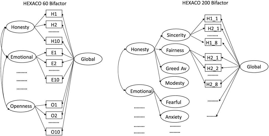
Partial illustration of bifactor model diagrams for HEXACO 60 and HEXACO 200. Note that all latent factors representing HEXACO domains were allowed to correlate. Baseline model was the same as the former except that the global factor was not included. The small number of within–domain/facet residuals are not shown in this diagram. A complete model specification reproducible in lavaan is provided in the online OSF repository.

A measurement invariance analysis was performed to examine the effect of progressively constraining parameters. An initial model without constraints (configural) was followed by progressive constraints on item loadings (weak), item intercepts (strong), item residuals (strict), latent factor variances (StrictVar) and latent factor covariances (StrictCov). In addition, a small number of within–domain (for the HEXACO–60 analysis) and within–facet (for the HEXACO–200 analysis) item residuals were allowed to correlate. To determine which correlated item residuals to include, single factor CFAs were estimated for each facet separately. Modification indices were obtained for all possible correlated residuals, and correlated residuals were included if their modification index was more than five MADs (median absolute deviation) above the median.

Sensitivity analyses presented in the online supplement showed that substantive inferences about changes in fit based on group–parameter constraints and inclusion of the global bifactor were robust to choices in model specification [i.e. maximum likelihood vs mean–adjusted and variance–adjusted weighted least squares (WLSMV) estimators, inclusion of correlated residuals, and using a subset of items or using all items]. The main conclusion was that WLSMV substantially increases absolute CFI values (i.e. .094 larger on average) but has minimal effect on RMSEA and SRMR. Because we focus on the comparative fit of the models, and because convergence failed for the WLSMV estimator for some models, we report the results of the maximum likelihood estimator. We also considered including an acquiescence factor; however, participants did not show any systematic tendency to agree. The mean on the 1 to 5 scale over all items and all participants was 2.98, which is very close to the scale midpoint of 3.

Initial analyses

Differences in means between applicants and non–applicants

Table 1 presents means and standard deviations on HEXACO domain and facet scores for applicants and non–applicants, as well as effect sizes (Cohen's d using pooled standard deviation) and tests of significant differences (two–tail independent groups t–tests). At the domain–level, applicants scored substantially higher on honesty–humility (d = 0.86), extraversion (d = 0.73), agreeableness (d = 1.06), and conscientiousness (d = 0.77). Although differences on emotionality (d = −0.14) and openness (d = 0.09) were statistically significant, these differences were small. At the facet–level, differences between applicants and non–applicants broadly aligned with respective domains with some noteworthy within–domain variation. In particular, among facets of emotionality, applicants scored lower on anxiety (d = −0.51) and higher on sentimentality (d = 0.24). More subtle examples of within–domain variation can be seen for openness where applicants scored higher on inquisitiveness (d = 0.21) and lower on unconventionality (d = −0.22). The average absolute standardized difference was 0.61 for domains and 0.50 for facets. In addition, detailed analyses presented in the online supplement suggest that reliability, factor structure, proportion of variance explained by the first component, and average absolute correlations were similar between applicants and non–applicants.

OPEN IN VIEWER

Table 1

Means, standard deviations and effect size (Cohen's d) of domain and facet scores for applicants and non–applicants

	Non–applicant		Applicant
Trait	M	SD	M	SD	d	Sig
Honesty–humility	3.66	0.44	4.01	0.37	0.86	***
Emotionality	3.02	0.43	2.97	0.35	−0.14	***
Extraversion	3.75	0.48	4.05	0.35	0.73	***
Agreeableness	3.17	0.45	3.60	0.36	1.06	***
Conscientiousness	3.69	0.43	3.99	0.35	0.77	***
Openness	3.54	0.48	3.58	0.41	0.09	**
H1: Sincerity	3.61	0.55	3.87	0.46	0.50	***
H2: Fairness	4.10	0.62	4.55	0.39	0.86	***
H3: Greed–avoidance	3.33	0.65	3.68	0.59	0.55	***
H4: Modesty	3.61	0.56	3.96	0.48	0.67	***
E1: Fearfulness	2.66	0.63	2.59	0.55	−0.11	**
E2: Anxiety	3.05	0.67	2.73	0.55	−0.51	***
E3: Dependence	2.88	0.60	2.93	0.50	0.09	*
E4: Sentimentality	3.50	0.56	3.62	0.46	0.24	***
X1: Social self–esteem	4.13	0.52	4.45	0.38	0.70	***
X2: Social boldness	3.59	0.65	3.85	0.49	0.44	***
X3: Sociability	3.43	0.65	3.77	0.49	0.59	***
X4: Liveliness	3.83	0.59	4.14	0.42	0.60	***
A1: Forgiveness	2.98	0.66	3.51	0.51	0.89	***
A2: Gentleness	3.10	0.55	3.46	0.47	0.70	***
A3: Flexibility	3.18	0.52	3.59	0.44	0.85	***
A4: Patience	3.40	0.61	3.84	0.48	0.79	***
C1: Organization	3.72	0.71	4.05	0.55	0.53	***
C2: Diligence	3.86	0.55	4.12	0.39	0.55	***
C3: Perfectionism	3.55	0.55	3.76	0.49	0.39	***
C4: Prudence	3.64	0.55	4.04	0.41	0.83	***
O1: Aesthetic appreciation	3.53	0.69	3.60	0.60	0.12	***
O2: Inquisitiveness	3.70	0.65	3.84	0.58	0.21	***
O3: Creativity	3.49	0.60	3.55	0.52	0.11	**
O4: Unconventionality	3.42	0.54	3.32	0.42	−0.22	***
I: Altruism	4.02	0.50	4.21	0.39	0.44	***

*

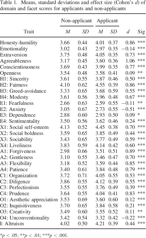
p < .05;

**

p < .01;

***

p < .001.

Item–level indicators of social desirability

An assumption of interpretation when applying a bifactor model to applicants and non–applicants is that loadings on the first unrotated factor (in both applicants and non–applicants) and item–level differences between applicants and non–applicants all reflect social desirability. Furthermore, item–level indicators in the instructed faking dataset provide a direct measure of social desirability. Descriptive statistics and intercorrelations for these item–level indicators are presented in Table 2 (see Table S1 in the online supplement for corresponding analysis of absolute indicators of item–level social desirability). Because correlations of item characteristics are almost identical for the 200–item and 100–item version of the HEXACO–PI–R, we focus discussion on 100–item version that allows for comparison with the instructed faking dataset. Importantly, loadings in the applicant and non–applicant samples were almost identical (i.e. r = .98), and correlations between loadings and standardized mean differences were very large (i.e. r = .86 and r = .89). These indicators from the current study correlated highly with direct measures of social desirability from the instructed faking study (i.e. applicant mean and standardized mean difference). Thus, results suggest that applicant loadings, non–applicant loadings and differences between applicants and non–applicants in the current study are all indexing item–level social desirability.

OPEN IN VIEWER

Table 2

Correlations between directed item–level indicators of social desirability

Item characteristic	M	SD	1	2	3	4	5	6	7	8	9
Current study
1. Non–applicant loading	−0.06	0.32		.98	.82	.90	.87
2. Applicant loading	−0.04	0.31	.98		.85	.93	.90
3. Non–applicant mean	2.98	0.68	.81	.84		.96	.68
4. Applicant mean	2.92	0.92	.90	.93	.96		.85
5. Standardized mean difference	−0.08	0.38	.86	.89	.68	.85
Instructed faking study
6. Non–applicant loading	−0.04	0.33	.94	.94	.75	.86	.89
7. Applicant loading	−0.01	0.42	.95	.95	.78	.88	.86	.94
8. Non–applicant mean	3.09	0.52	.55	.62	.87	.80	.50	.52	.54
9. Applicant mean	3.06	0.85	.86	.91	.94	.96	.78	.84	.89	.85
10. Standardized mean difference	−0.06	0.23	.89	.90	.73	.82	.80	.88	.94	.45	.84

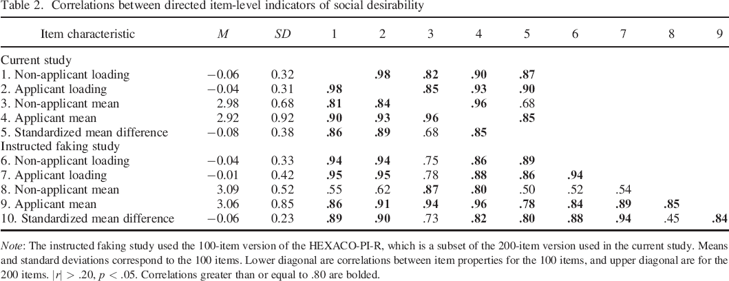
Note: The instructed faking study used the 100–item version of the HEXACO–PI–R, which is a subset of the 200–item version used in the current study. Means and standard deviations correspond to the 100 items. Lower diagonal are correlations between item properties for the 100 items, and upper diagonal are for the 200 items. |r| > .20, p < .05. Correlations greater than or equal to .80 are bolded.

Bifactor models

Table 3 present the model fit statistics and important parameters for the invariance test of the baseline and bifactor models for the 200–item HEXACO–PI–R. Models were also estimated for the 60–item HEXACO–PI–R (Table S4) and the relative pattern of fit statistics for invariance constraints was similar to the 200–item version. In terms of the invariance tests, constraining item loadings and item intercepts led to only minor reductions in fit (e.g. reduction in CFI of around .01). In contrast, constraining item residuals led to a dramatic reduction in fit, the implications of which are discussed in the next section. Constraining latent factor variances and covariances to be equal resulted in only small reductions in fit. Overall, the bifactor model resulted in a substantial improvement in model fit relative to the baseline model (i.e. increase in CFI of around .05).

OPEN IN VIEWER

Table 3

Model fit statistics for invariance tests on baseline and Bifactor models applied to HEXACO 200 item version of the HEXACO–PI–R

	Fit statistics					Parameters
Model	χ2	df	CFI	RMSEA	SRMR	RN	RA	MAD	DC	DG
Baseline
Configural	97680	39021	.728	.031	.069	.38	.38
Weak (L)	98624	39217	.725	.031	.070	.36	.39
Strong (LI)	102221	39386	.709	.031	.070	.37	.40	0.66	0.88
Strict (LIR)	110962	39586	.669	.033	.072	.38	.39	0.68	0.89
StrictVar (LIRV)	113305	39617	.659	.034	.090	.32	.55	0.57	0.75
StrictCov (LIRVC)	113718	39632	.657	.034	.079	.38	.38	0.58	0.76
StrongVar (LIV)	103605	39417	.703	.032	.086	.32	.54	0.57	0.75
StrongCov (LIVC)	103977	39432	.701	.032	.076	.39	.39	0.59	0.77
Bifactor
Configural	85640	38621	.782	.027	.053	.16	.19
Weak (L)	87407	39016	.776	.028	.056	.13	.20
Strong (LI)	89428	39184	.767	.028	.057	.13	.20	0.26	0.30	1.31
Strict (LIR)	98484	39384	.726	.031	.059	.13	.20	0.27	0.32	1.30
StrictVar (LIRV)	100734	39416	.716	.031	.071	.12	.27	0.25	0.29	1.10
StrictCov (LIRVC)	100991	39431	.715	.031	.068	.16	.16	0.25	0.29	1.10
StrongVar (LIV)	90844	39216	.761	.029	.067	.12	.25	0.23	0.26	1.12
StrongCov (LIVC)	91048	39231	.760	.029	.064	.16	.16	0.23	0.26	1.12

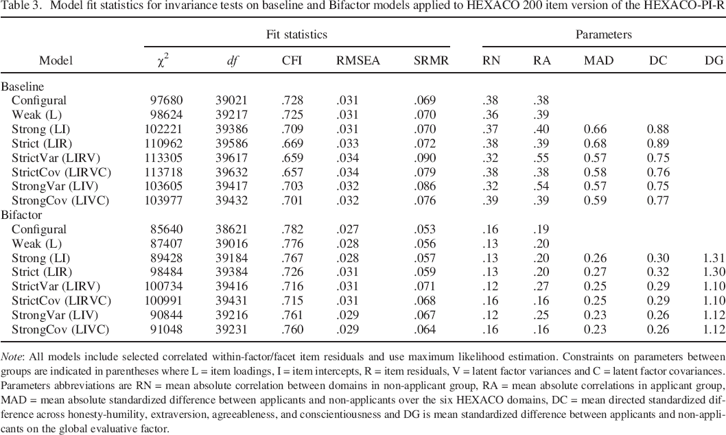
Note: All models include selected correlated within–factor/facet item residuals and use maximum likelihood estimation. Constraints on parameters between groups are indicated in parentheses where L = item loadings, I = item intercepts, R = item residuals, V = latent factor variances and C = latent factor covariances. Parameters abbreviations are RN = mean absolute correlation between domains in non–applicant group, RA = mean absolute correlations in applicant group, MAD = mean absolute standardized difference between applicants and non–applicants over the six HEXACO domains, DC = mean directed standardized difference across honesty–humility, extraversion, agreeableness, and conscientiousness and DG is mean standardized difference between applicants and non–applicants on the global evaluative factor.

For parameter interpretation, we focus on the strong models where item–level intercepts and factor loadings were constrained to be equal between groups. Specifically, we examined the degree to which applicant response distortion was captured by the global factor in the bifactor model. First, we note that loadings on the global factor in the bifactor model were highly correlated with other item–level indicators of social desirability. Specifically, bifactor loadings correlated .95 with applicant loadings, .88 with applicant mean, .90 with applicant–non–applicant Cohen's d and .86 with Cohen's d in the instructed faking study. Second, averaging over the four scales that showed the largest differences between applicants and non–applicants (i.e. honesty–humility, extraversion, agreeableness, and conscientiousness), the mean standardized difference for these four latent factors was 0.88 (baseline) and 0.30 (bifactor). Thus, averaged across these four domains, the effect of the applicant context on latent scale mean differences was substantially reduced, although not removed entirely, in the bifactor model compared with the baseline model. Consistent with the global factor absorbing much of domain–level differences, applicants scored 1.31 standard deviations higher on the latent global factor in the bifactor model.

Further analyses examined the degree to which the inclusion of the evaluative factor explained correlations between the six HEXACO domains. Table 4 presents the correlations between domain scores in the applicant and non–applicant samples using observed scores and latent domain scores from the strong models (i.e. item loadings and intercepts constrained to be equal). Both the baseline model and the observed score correlations show a clear pattern of correlations consistent with a socially desirable global factor of personality. ¹ In contrast, the pattern of correlations in the bifactor model was substantially altered. In particular, the average absolute correlation between the six latent variables representing the six HEXACO domains went from .37 (baseline) to .13 (bifactor) for non–applicants and from .40 (baseline) to .20 (bifactor) for applicants. Furthermore, the pattern of correlations between substantive factors in the bifactor model showed little alignment with a global factor (Table 4). Thus, the bifactor model essentially provides an alternative representation of the common item–level variance.

OPEN IN VIEWER

Table 4

Bivariate correlations among the HEXACO domain scores for applicants (upper diagonal) and non–applicants (lower diagonal)

Measure	H	E	X	A	C	O	Mean abs r
Observed Scores
Honesty–humility		.06	.09	.37	.21	.07
Emotionality	−.03		−.25	−.18	−.07	−.11
Extraversion	.15	−.24		.39	.41	.33
Agreeableness	.34	−.21	.34		.35	.24
Conscientiousness	.28	−.16	.31	.19		.16
Openness	.13	−.13	.30	.16	.11

Mean abs r							.21 1 / .22 2
Baseline Latent Factors
Honesty–humility		−.12	.38	.55	.57	.20
Emotionality	−.17		−.45	−.47	−.30	−.13
Extraversion	.34	−.47		.61	.70	.38
Agreeableness	.50	−.48	.52		.58	.33
Conscientiousness	.51	−.40	.57	.40		.26
Openness	.27	−.15	.34	.23	.21

Mean abs r							.37 1 / .40 2
Bifactor Latent Factors
Honesty–humility		.34	−.36	.22	−.02	−.03
Emotionality	.29		.10	.04	.22	.13
Extraversion	−.34	.16		.32	.33	.28
Agreeableness	.17	.04	.16		.32	.19
Conscientiousness	−.05	.10	.11	.01		.08
Openness	.08	.14	.22	.06	.02
Mean abs r							.13 1 / .20 2

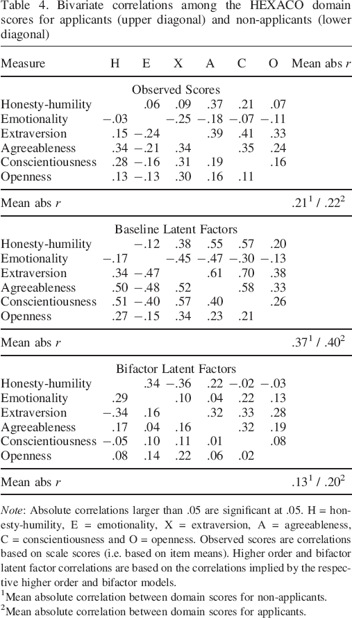
Note: Absolute correlations larger than .05 are significant at .05. H = honesty–humility, E = emotionality, X = extraversion, A = agreeableness, C = conscientiousness and O = openness. Observed scores are correlations based on scale scores (i.e. based on item means). Higher order and bifactor latent factor correlations are based on the correlations implied by the respective higher order and bifactor models.

1

Mean absolute correlation between domain scores for non–applicants.

2

Mean absolute correlation between domain scores for applicants.

Overall, the bifactor model appeared to achieve superior model fit by being better at representing differences in item–level social desirability within traits. While the general orientation of item–level social desirability tended to be fairly consistent within factors (e.g. most positively worded conscientiousness items are socially desirable, and most negative worded conscientiousness items are socially undesirable), the degree of social desirability did vary. For instance, for 93% of items, the loading on the global factor was in the same direction as the loading on the broad trait (after reversing emotionality). However, illustrating the variability in degree of item social desirability loadings, whereas loadings on the bifactor had a mean of .27, the standard deviation was .16. Thus, the bifactor model may achieve superior fit by being better able to represent within–factor and within–facet variation in social desirability.

Model invariance testing indicated that constraining item–level residuals to be equal for applicants and non–applicants led to a substantial reduction in model fit (Table 3; strong vs strict model fits). One explanation for this finding is that elevated levels of social desirability result in a movement to an ideal response rather than a systematic increase. Several analyses indicated that applicant responses showed less variation than non–applicant responses. The mean of the square root of item–level error variances in the 200–item strong models was examined. The ratio of applicant to non–applicant values was 0.885 for the baseline model and 0.882 for the bifactor model. Similarly, the mean ratio of applicant to non–applicant item standard deviations was 0.83. Naturally, smaller item standard deviations translated into smaller scale score standard deviations. Averaged over the 25 facets, applicant standard deviations were significantly smaller (p < .01, for all facets, using Levene's test); on average applicant standard deviations were only 0.80 of non–applicant standard deviations (SD = 0.07, range: 0.63 to 0.91). Because standard deviations tend to decrease as means gets closer to scale endpoints, we calculated a relative standard deviation for each facet for applicants and non–applicants by dividing the obtained standard deviation by the maximum possible standard deviation given the mean (Mestdagh et al., 2016). For function details, see the relative SD function in the online repository. The greater proximity of facet means to scale endpoints in the applicant context only explained around a fifth of the observed reduction in standard deviation. Specifically using relative standard deviations, the mean ratio of applicant to non–applicant standard deviations was still only 0.85 (SD = 0.05, range: 0.77 to 0.95). Further analysis on the actual model parameters suggested that the variation in the latent variables was also smaller. Specifically, looking at the strong bifactor HEXACO–200 model, the ratio of standard deviations on the latent global factor (applicants/non–applicants) was 0.74 and for the latent domain factors was 0.84. Thus, reduced variability in latent social desirability was even greater than for the substantive traits.

Social desirability and higher order structure

The results broadly converge with other research suggesting that correlations between higher order factors are caused by item–level social desirability effects (Bäckström et al., 2009; Ziegler & Buehner, 2009). First, inclusion of the evaluative factor in the bifactor model substantially reduced correlations between broad traits, and the correlations that remained were not reflective of the GFP (i.e. social effectiveness or social desirability). Importantly, the bifactor model provided a substantial improvement in fit over the baseline model. Furthermore, loadings on the evaluative factor were almost synonymous with other indicators of social desirability. For example, loadings on the evaluative factor in the bifactor model and loadings on the first component for both non–applicants and applicants correlated highly with direct measures of item social desirability such as differences between applicants and non–applicants.

Consistent with the work of Biderman and colleagues (Biderman et al., 2011; Chen et al., 2016), the GFP as higher order factor can be understood as the result of an item–level process. A contribution of the present study is to present ample evidence that this factor corresponds to social desirability. In particular, the focus on GFP as a higher order factor has been perpetuated by analyses performed on scale scores rather than items. Of course, some discussion of the GFP has been fuzzy about the distinction between whether the GFP is an item–level process or a higher order construct. And some researchers have extracted the first unrotated factor using item–level data and labelled this the GFP (Musek, 2007). However, assuming these loadings are indexing social desirability, it seems more appropriate to describe such a factor as social desirability. Future research might consider constraining the loadings of the evaluative factor, so they correspond to externally derived estimates of item social desirability. This would further remove the ambiguity of whether a general factor is a pure or a contaminated measure of social desirability.

We also note that for many measures of personality, including the HEXACO–PI–R, there is strong alignment between the social desirability of the factor and the social desirability of items within that factor. For example, most conscientiousness items are written in a socially desirable way. As such, we would expect greater differences between a higher order and a bifactor model for questionnaires with greater within–factor variation in item social desirability. It is also interesting to consider how this social desirability factor might be influencing questionnaire development and construct definition. In particular, aligning substantive traits with social desirability may yield stronger factor loadings and scale reliabilities, at the expense of reduced predictive validity due to non–orthogonal factors. In particular, future research could examine whether the superiority of the bifactor model over a standard correlated factor model is increased when using questionnaires with either more subtle items or with items that are deliberately designed to have varying levels of social desirability within a given factor.

Although the present research reinforces the importance of modelling social desirability at the item–level, it does not resolve the ongoing debate about whether it reflects substance or bias (Chen et al., 2016; McCrae & Costa, 1983). Chen et al. (2016), who also employed an item–level bifactor approach, labelled the general factor, the ‘M’ factor, to reflect the ambiguity over whether it reflects method or meaning. They presented initial evidence that the evaluative factor correlates across self and other ratings. This parallels findings in the literature on social desirability scales (McCrae & Costa, 1983). It would also be strange if this major source of variance in measures of personality did not index at least some substantive variance. Changes in the applicant context show that levels of social desirability can be temporarily altered by context, but it is likely that a reasonable percentage of social desirability in non–applicant contexts reflects substance rather than bias. While Chen et al. (2016) provide some initial estimates, it would be useful for future research using large samples to re–examine the issue of self–other agreement using the item–level bifactor approach.

Response distortion in job applicants

We agree with Klehe et al. (2012) that the bifactor model can explain a diverse range of underlying processes that give rise to various degrees of socially desirable responding. For example, qualitative studies using talk–aloud protocols (Robie, Brown, & Beaty, 2007; Ziegler, 2011) and within–person studies looking at difference scores between applicants and non–applicants (Griffith, Chmielowski, & Yoshita, 2007) suggest that job applicants can be broadly classified into honest responders, slight fakers and extreme fakers. Slight fakers tweak their honest responses to be more socially desirable, whereas extreme fakers respond mostly in terms of social desirability. The assumption of the bifactor model is that despite diverse cognitive processes influencing responses to items, the effect of these different processes will largely be explained by a person's score on the socially desirability factor.

The bifactor model implies that a unitary concept of social desirability is sufficient. This is inconsistent with many multifaceted theories of social desirability. For instance, Paulhus (1986) has distinguished between implicit (i.e. self–deception) and explicit (i.e. impression management) processes of response distortion. Other researchers have examined whether applicants tailor responses to job requirements, which implicitly assumes that the meaning of social desirability varies between work and general contexts and between different jobs (Dunlop et al., 2012). The present research does not preclude the existence of multifactorial models of social desirability; it merely suggests that the main effect can be explained by a single factor. Supporting this claim, Dunlop et al. (2012) had participants’ rate item social desirability across four different job contexts (i.e. nurse, used car sales person, fire fighter and general job). While they did find a few significant job by scale point interactions, in a re–analysis, we calculated that over the items, the average main effect of scale point explained 45% of variance while the job by scale point interaction only explained 6% and this is without corrections for the larger degrees of freedom associated with the interaction (i.e. 12) than the main effect (i.e. 4). Thus, although more research is needed, perhaps 90% or more of social desirability effects generalize across jobs. That said, it may be more parsimonious and clear to constrain loadings on the evaluative factor in the bifactor model to correspond to direct measures of social desirability.

The bifactor model may also explain differences in effect sizes across scales and across studies when comparing applicants and non–applicants (Birkeland et al., 2006). From this perspective, scale–level effect sizes result from the combined effect of item–level social desirability characteristics and the distribution of contextually influenced person–level social desirability. At the item–level, scales differ substantially in how much their constituent items are socially desirable. At the person–level, a wide range of factors influence how much a given applicant sample decides to distort their responses. The bifactor model allows for some mechanisms such as objective or subtle items (Bäckström et al., 2009) to influence item–level social desirability, and contextual factors such as warnings and the job market to influence person–level social desirability (McFarland & Ryan, 2006). Future research could seek to obtain a large number of datasets from the published literature to examine the applicability of such a parsimonious model.

The bifactor model also provides a means of revisiting discussion about the effectiveness of corrections for social desirability (McCrae & Costa, 1983; Uziel, 2010). The general conclusion of research looking at correcting for social desirability is that it removes at least as much substance as it does bias, and that it does not increase, and may even decrease, self–other correlations and predictive validity (McCrae & Costa, 1983). In general, the evaluative factor in the bifactor model correlates very highly with other methods for estimating social desirability. As such, it is likely to have similar limitations and corrections using the bifactor model are unlikely to immediately solve the issue of correcting for response distortion. In general, more work is needed using bifactor models to better understand the issue of substance versus bias. In particular, large studies that examine self–other correlations and predictive validity will be useful. Future research could also study questionnaires where each trait includes items with a greater variance in social desirability in order to reduce the collinearity between broad traits and social desirability. Finally, within–person studies of applicant and non–applicant responses and further modelling of quadratic social desirability effects should help in separating bias and substance components in social desirability.

Interestingly, consistent with past research (Hooper & Sackett, 2007), the standard deviation of scales at both domain and facet–level was around 20% lower in the applicant sample. We propose several explanations for this. First, results showed that around a quarter of this reduction can be attributed to floor and ceiling effects related to the mean in applicant samples moving toward scale end points. Second, in line with De Vries, Realo, and Allik (2016), we argue that socially desirable responding is fundamentally an item–level process. Items for a given facet vary in their social desirability, which in turn may lead to dampening or even counteracting effects at the facet–level when some items are formulated neutrally or even opposite to each other with respect to social desirability. This effect is amplified at the domain–level, where even greater diversity in item–level social desirability should be observed because both facets and items within facets may differ in the extent to which socially desirable responding becomes activated. Third, it seems likely that faking is positively skewed such that applicants who are in actuality lower on a socially desirable item or trait are likely to increase their score more than an applicant who is in actuality already close to the socially desirable ideal. This differential degree of socially desirable responding results in a compression of scores around the ideal and a smaller standard deviation. Finally, the effect of social desirability may plateau or decline before as response options move from ‘agree’ to ‘strongly agree’ (Dunlop et al., 2012). In such instances, socially desirable responding may involve moving to an optimal point rather than a fixed increase. Of all these effects, we think that the relatively greater increase by those who normally score low on social desirability is the major cause of the observed reduction in standard deviation. Further modelling work should seek to integrate quadratic models of social desirability into item–level bifactor models. While the bifactor suggests that variance on the evaluative factor was reduced in the applicant sample, this may be an artefact of quadratic social desirability.

Hexaco Personality Inventory in Employee Selection

The present study is also particularly relevant to employers wishing to use the HEXACO–PI–R in a selection context. Research has generally reinforced the value of the HEXACO model of personality in predicting workplace outcomes (Ashton et al., 2014; Ashton & Lee, 2008; De Vries et al., 2016). The present study shows that the pattern of response distortion on the HEXACO–PI–R differs from what is typically seen in Big Five meta–analytic literature (Birkeland et al., 2006). Specifically, response distortion was greater on HEXACO agreeableness and lower on HEXACO emotionality than their Big Five analogues. The high levels of response distortion on agreeableness may be due to the elements of anger and aggression that constitutes its negative pole. The lower levels of response distortion on HEXACO emotionality, as compared with Big Five neuroticism, may be due to the reduced emphasis on negative emotions such as stress and anger and the increased emphasis on more neutral traits such as dependence and sentimentality. The substantial response distortion seen on honesty–humility may be explained by its emphasis on integrity and professional ethics. This becomes even clearer when we consider that low scores on honesty–humility indicates deceptiveness, arrogance and greed, as evident by it being almost identical to the general trait underlying the dark triad (Lee & Ashton, 2014).

In addition, applicant response distortion on the HEXACO–PI–R (often in the range, d = 0.7 to 1.1) was larger than seen in meta–analyses of applicant behaviour (Birkeland et al., 2006). There are several possible explanations for this. First, the HEXACO–PI–R is a 200–item questionnaire. Such lengthy questionnaires allow for more reliable measurement and therefore greater response bias. Second, the questionnaire was designed as a general measure of personality where participants are assumed to be co–operative. It uses a normative response format rather than an ipsative response format (Heggestad, Morrison, Reeve, & McCloy, 2006), and it does not explicitly attempt to use evaluatively neutral items (Bäckström et al., 2009). In both these respects (reliability and transparency), the HEXACO–PI–R shares similarities with the NEO PI–R, and studies using the NEO PI–R comparing applicants and non–applicants have obtained similar levels of response distortion to the present study (i.e. in the range of one standard deviation, Marshall, De Fruyt, Rolland, & Bagby, 2005).

Interestingly, other structural features of the HEXACO–PI–R, including factor loadings, scale reliabilities, and indicators of the importance of the global factor such as average absolute domain correlations, were fairly similar across applicant and non–applicant samples. There are several explanations for how substantial response distortion can co–exist with limited change to other test properties. Much of this can be explained in terms of response biases being an item–level process that is in some respects a fixed effect that operates at the item–level and is proportional to the gap between actual and ideal, such that applicants who would honestly respond with low social desirability show greater response distortion in applicant settings and those that are already close to the ideal show much less response distortion.

Facet–level models

The present study also contributes to attempts to model complex hierarchical measures of personality. This is important given that almost all large sample studies using appropriate data analytic approaches (Anglim & Grant, 2014) find that regression models with narrow traits provide modest but meaningful incremental prediction of important outcomes (Anglim & Grant, 2016; Anglim, Knowles, Dunlop, & Marty, 2017; Ashton, 1998; Christiansen & Robie, 2011; De Vries, De Vries, & Born, 2011; Dudley, Orvis, Lebiecki, & Cortina, 2006; Hogan & Roberts, 1996). Nonetheless, only a few past studies have explicitly examined job applicant response distortion at the facet–level (Marshall et al., 2005). Consistent with Ziegler et al. (2010), we found that mean differences at the facet–level showed substantial variability within some domains. The study also provides a demonstration of how item–level models can be applied to model the full hierarchical measures at the item–level. Item parcelling (Bandalos, 2002; Little, Cunningham, Shahar, & Widaman, 2002) simplifies analysis, makes it easier to satisfy common rules of thumb for fit measures and provides a quick way to get a basic estimate of a latent variable. However, if researchers are interested in the fundamental structure of personality, it is essential that latent variable modelling is performed at the item–level. This is especially important where the effect of factors such as social desirability operates differentially over items.

We obtained similar results whether fitting models to the HEXACO–60 at the domain–level or the full hierarchical structure of the HEXACO–200. In general, specifying full hierarchical models introduces several challenges, which may explain the paucity of research. They require bigger samples to estimate. They take longer to specify accurately. They take longer to estimate (some of our models took around 30 minutes to estimate). They are more likely to encounter convergence issues, and when problems arise, they are harder to diagnose. However, none of these challenges are justification for not performing analysis at the item–level. Hopefully, with the rise of open science and the emphasis on data sharing, more researchers in personality will choose to share item–level data and not just scale–level data.

Limitations and future research

A major challenge when comparing applicants and non–applicant is determining whether the differences reflect the effect of the applicant context or underlying substantive differences. In the present study, we used matching on age and gender to increase underlying similarities. We were also able to verify using follow–up data in an ‘honest’ research setting that differences between groups largely disappeared. We also showed that differences were in the direction implied by item–level social desirability. More generally, the large observed differences (i.e. around one standard deviation) are likely to dwarf any small remaining substantive differences, and the large sample sizes meant that uncertainty in effect estimation was small.

Second, building on the work of Biderman and colleagues (Biderman et al., 2011; Chen et al., 2016), the present study highlights a wide range of potential follow–up studies that could apply item–level bifactor models. Research examining convergence of GFP estimates across different personality questionnaires could be re–examined using an item–level approach (Hopwood, Wright, & Donnellan, 2011; Van der Linden, Tsaousis, & Petrides, 2012). Because social desirability mainly acts at the item level, we would expect larger correlations when using an item–level approach, and even larger correlations where loadings are specified to align with item–level social desirability evaluations.

Third, there is a need for formal integrated mathematical models of applicant response distortion. In particular, it would be good to extend the bifactor model to appropriate within–person data where participants are measured in both applicant and non–applicant settings. Various simulation models have been developed to describe applicant response distortion at the scale–level (Komar, Brown, Komar, & Robie, 2008). However, item–level response distortion is likely to result in particular patterns of scale–level change, and there is a need to be able to estimate parameters of such models using within–person data. Ziegler, Maaß, Griffith, and Gammon (2015) present additional strategies for modelling response sets and latent classes in applicant settings that could complement the current bifactor approach.

Fourth, although analyses of directed item–level social desirability showed very strong convergence across indicators, these correlations were substantially weaker when examining absolute indicators (see online supplement). The method of correlating loadings with criteria is known in the intelligence literature as the method of correlated vectors. This method has received substantial criticism (Wicherts, 2017; Wicherts & Johnson, 2009). In particular, a range of sample characteristics such as item means and standard deviations can constrain observed loadings. In the case of directed social desirability, these effects appear to be minor relative to the general tendency for an item to be desirable or undesirable. However, future research could further refine understanding of how these methodological artefacts alter the precision of factor loadings in providing absolute indicators of item social desirability.

Finally, we also note the methodological literature grounded in intelligence research has provided advice on and critically discussed comparing bifactor and correlated factor models (Gignac, 2007, 2016; Murray & Johnson, 2013). For example Murray and Johnson (2013, p. 409) suggest that the ‘bi–factor model may simply be better at accommodating unmodelled complexity in test batteries’. We present several arguments to suggest that this is not the case in the present study. First, loadings on the evaluative factor in the bifactor model correlated highly with other item–level indicators of social desirability. Thus, the unmodelled complexity captured by the evaluative factor seems to be mainly social desirability, and that is what the model is intended to capture. Second, perhaps in contrast to the intelligence literature, item loadings on social desirability vary substantially within latent traits. This further explains the substantial improvement in fit achieved by the bifactor model over the correlated factor model. Finally, the bifactor model is theoretically grounded in a theory of how traditional traits and social desirability combine to influence item responses. Nonetheless, future work could further examine the statistical properties of the bifactor model in the context of personality measurement. Simulation studies using different data generating mechanisms could assist in clarifying the evidence provided by bifactor models.