Characteristics of advanced high-strength steels obtained by the compact strip production route

Introduction

Regulations imposed to reduce fuel consumption, and their corresponding effect on emission of green-house gases, in light and heavy-duty vehicles, have promoted the development of materials with enhanced mechanical properties that are used in the manufacture of structural components. Such improvement in fuel consumption will result as consequence in diminishing the weight and size of components manufactured with better and stronger materials [1,2]. The iron and steel industry has responded by offering advanced high-strength steels (AHSS), in which chemical composition and processing conditions are tailored to obtain various microstructures made of a wide range hard and soft components that are responsible for enhancing their strength [3,4].

AHSS are cast, hot-rolled, cooled in the run-out table and coiled [3,4]. Most of these steels are cast in conventional moulds where the surface freezes rapidly, while the centre solidifies at a lower rate. Such differences in cooling and solidification rates promote the enrichment of alloying elements towards the centre of the slab in what is known as central segregation, or macrosegregation, that cannot be removed from the final product due to the high temperatures and long times required to homogenise the steel by diffusion [5,6]. It has been reported that central segregation enhances the yield and ultimate strength of the steel, but affects in a negative way its formability, ductility and impact toughness [7-12].

An alternative to casting in conventional moulds is that of thin-slab casting in which the steel is poured into moulds that produce slabs that range from 50 to 90 mm in thickness, in contrast to conventional moulds that produce slabs of 250–350 mm. The faster solidification rate that takes place within thinner sections promotes microstructural refining and the reduction of the central line segregation [13-15]. A further advantage that the thin-slab casting technology offers is the reduction of size of the processing line by connecting the caster with continuous reheating furnaces and the rolling-mill [15-18]. The surface quality of the rolled strip is assured by the design of descaling practice that takes place before the stock enters the rolling mill [18].

The aim of this work is to study the behaviour of samples from two different AHSS produced by the thin-slab route; the microstructure was analysed by microscopical techniques, their mechanical behaviour was studied by means of tension tests conducted along three different directions in hot-rolled sheets. The stress–strain curves were fitted to different constitutive equations. This study was conducted as these steels are demanded by the automotive industry to reduce the weight and fuel consumption of vehicles without affecting safety uses.

Experimental procedure

The microstructure and mechanical properties of two AHSS, which will be identified in this work as A and B steels, were studied in their hot-rolling conditions. The chemical composition of both steels is shown in Table 1. The steel strips studied were in their hot-rolled condition and had a nominal thickness of 3.6 mm. Three tensile samples from both steels were cut and machined along the rolling, at 45° to it and transversal directions, which will be identified as 0°, 45° and 90° to the rolling direction. The dimensions of the tensile samples were of 12.7 mm in width and 50 mm in gauge length; the samples were tested following the ASTM E8/E8M standard [19].

OPEN IN VIEWER

Table 1

Chemical composition of the steels (% mass).

Steel	C	Mn	P	S	Cu	Ni	Si	Cr	Al	Ti	Mo	N
A	0.065	1.871	0.014	0.002	0.079	0.178	0.532	0.831	0.041	0.015	0.268	0.0074
B	0.056	1.123	0.008	0.002	0.085	0.035	0.257	0.067	0.053	0.141	0.042	0.0092

A commercial thermodynamic and kinetics computer program [20] was used to study the solidification kinetics and the continuous cooling transformation (CCT) diagram of the steel to deduce the feasibility of encountering different microstructural components expected to occur within the strips. Different computer models were used to evaluate the microstructural and thermal conditions within the steels as they were hot-rolled and cooled through the run-out table [16,17,21,22].

Samples from both steels were prepared for their microstructural observation by light optical and scanning electron microscopy (LOM and SEM, respectively). SEM observations were made in secondary and back-scattered electron (SE and BE, respectively) modes as well as selected energy-dispersive X-ray spectroscopy (EDX) analyses. Some samples were prepared for their observation by means of electron back-scattered diffraction (EBSD) to identify the various microstructural constituents [23].

Results

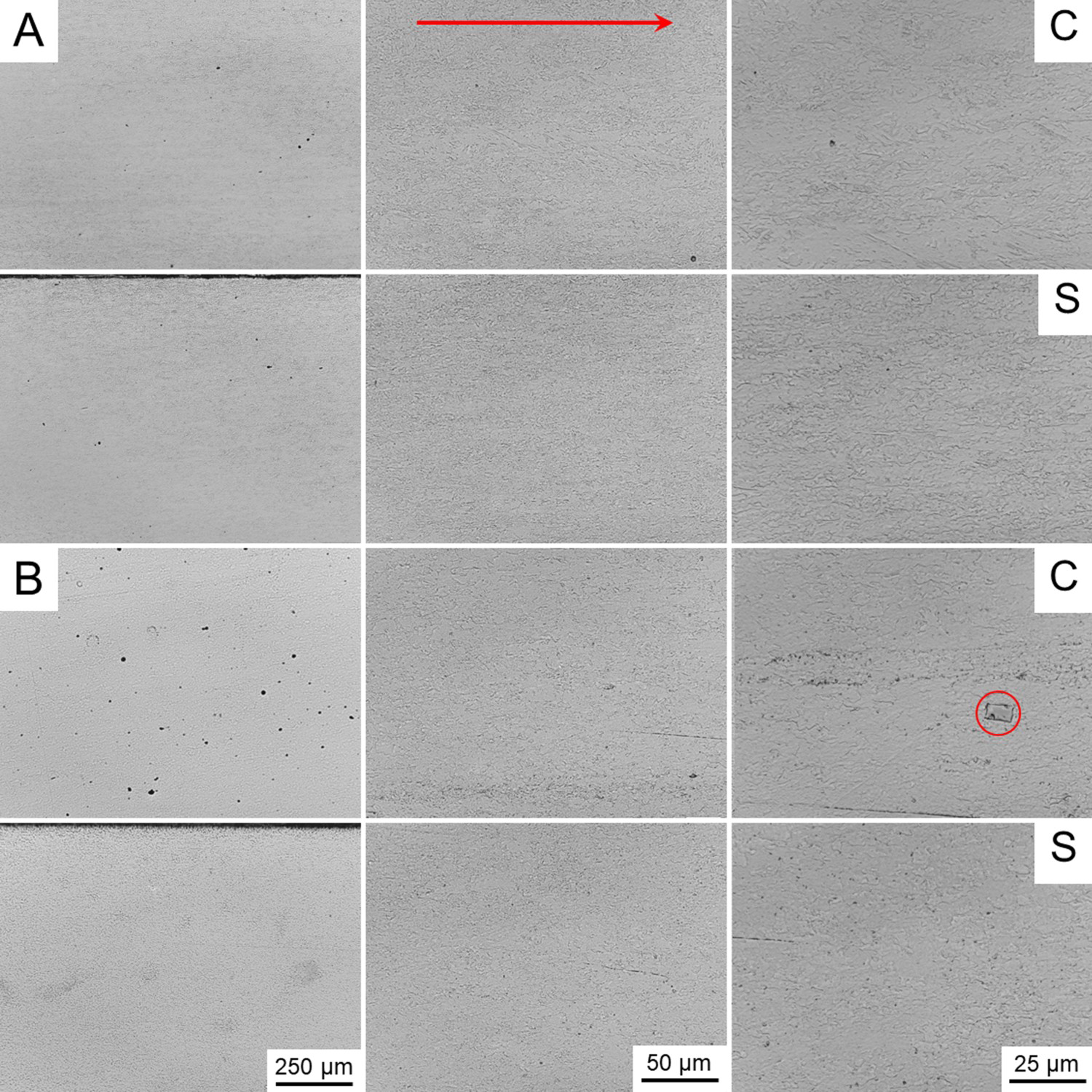
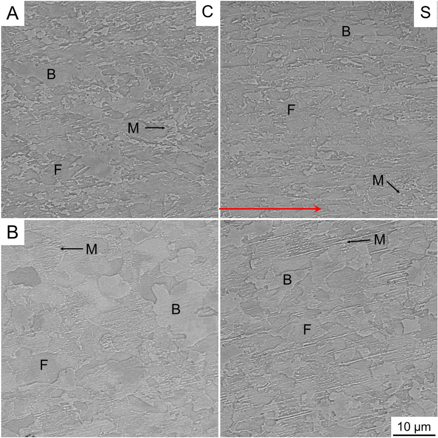
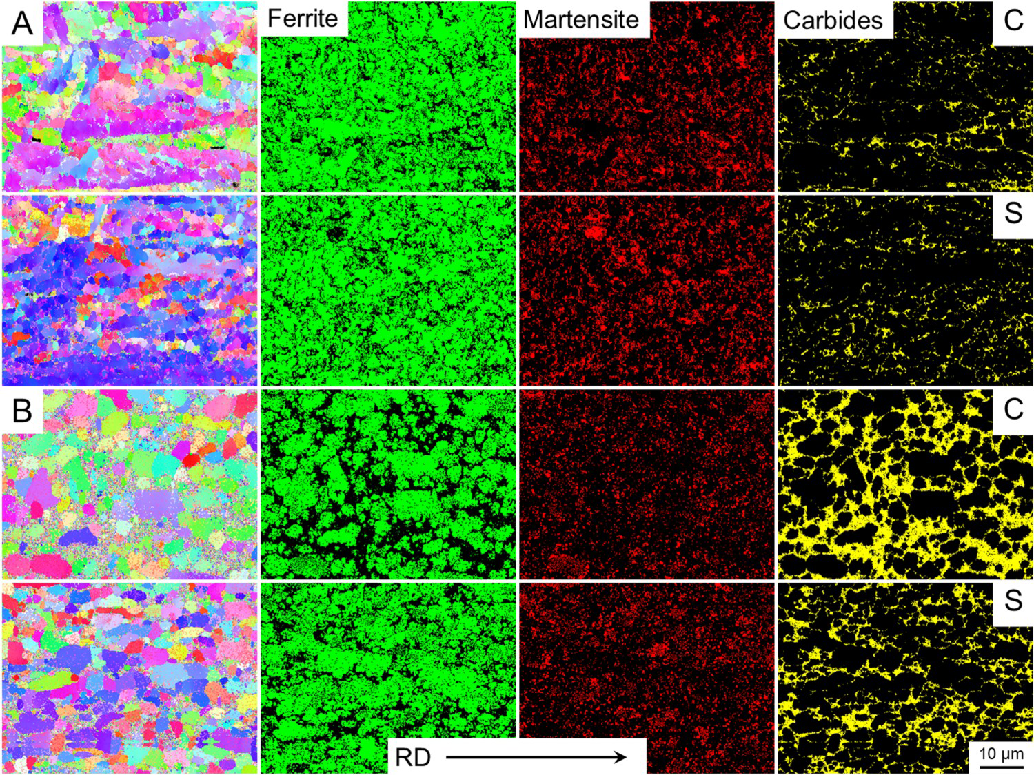
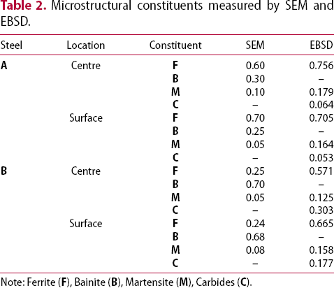
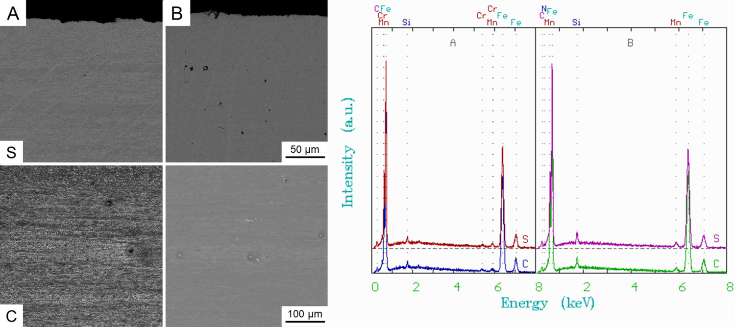
The chemical composition of the steels, Table 1, suggests that the strategy followed to achieve the required mechanical properties differs in either steel. The amount of carbon in either case is similar as both were cast in thin slab moulds and the peritectic composition is avoided [24,25]. Steel A has a higher content on alloying elements such as Mn, Si, Cr, Ni and Mo that will retard the transformation of austenite after hot rolling [3,4,26]; steel B is alloyed with Mn and Si, to retard the transformations, and contains higher amounts of N and Ti to strengthen by precipitation of TiN particles [12,27]. Figure 1 shows the microstructures observed by means of LOM of both steels towards the centre and surface of the strips at different magnifications. The rolling direction is indicated by the arrow. The microstructural finesse in both samples does not allow identifying different constituents, although a cuboid precipitate is pointed out towards the centre of strip B; EDX by SEM shows that such precipitates are made of TiN, as will be discussed later. Figure 2 shows SEM in SE micrographs for both steels in regions close to the centre and to the surface, the microstructural constituents that were identified were ferrite (F), bainite (B) and martensite (M), the rolling direction is indicated. Figure 3 shows images corresponding to the EBSD analyses of samples from steels A and B in locations close to the surface of the strip and at their centres, it was possible to identify the presence of martensite (M), carbides (C) and ferrite (F), but it was not possible to differentiate if this last component formed part of bainite or ferrite. The volume fractions of the different constituents are shown in Table 2. EDX area analyses were conducted towards the centre and close to the surface in both types of steels to discern about the tendency for central segregation. Figure 4 shows SE images from SEM of steels A and B close to the centre (C) and surface (S), the EDX spectra shown in this figure confirm the absence of such segregation.

OPEN IN VIEWER

Figure 1

LOM images of steels A and B at their centre (C) and close to the surface of the strip (S) at different magnifications. The rolling direction and a cuboid particle towards the centre of steel B are indicated.

OPEN IN VIEWER

Figure 2

SEM images of steels A and B at their centre (C) and close to the surface of the strip (S). The constituents indicated correspond to ferrite (F), bainite (B) and martensite (M); the rolling direction is indicated.

OPEN IN VIEWER

Figure 3

Images from steels A and B in regions close to the surface (S) and centre (C) of the strips. The analyses put in evidence the presence of ferrite, martensite and carbides. The rolling direction (RD) is indicated.

OPEN IN VIEWER

Table 2

Microstructural constituents measured by SEM and EBSD.

Steel	Location	Constituent	SEM	EBSD
A	Centre	F	0.60	0.756
		B	0.30	–
		M	0.10	0.179
		C	–	0.064
	Surface	F	0.70	0.705
		B	0.25	–
		M	0.05	0.164
		C	–	0.053
B	Centre	F	0.25	0.571
		B	0.70	–
		M	0.05	0.125
		C	–	0.303
	Surface	F	0.24	0.665
		B	0.68	–
		M	0.08	0.158
		C	–	0.177

Note: Ferrite (F), Bainite (B), Martensite (M), Carbides (C).

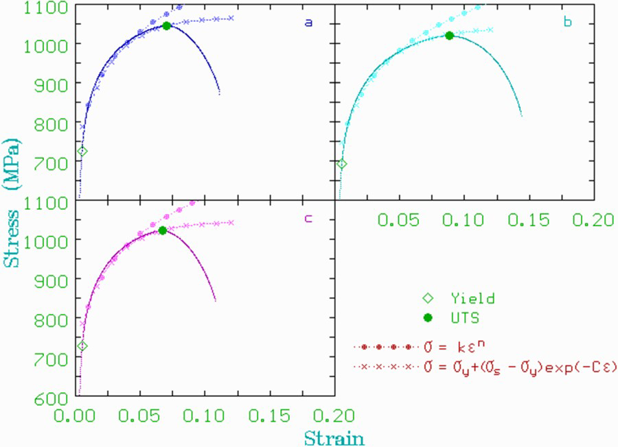
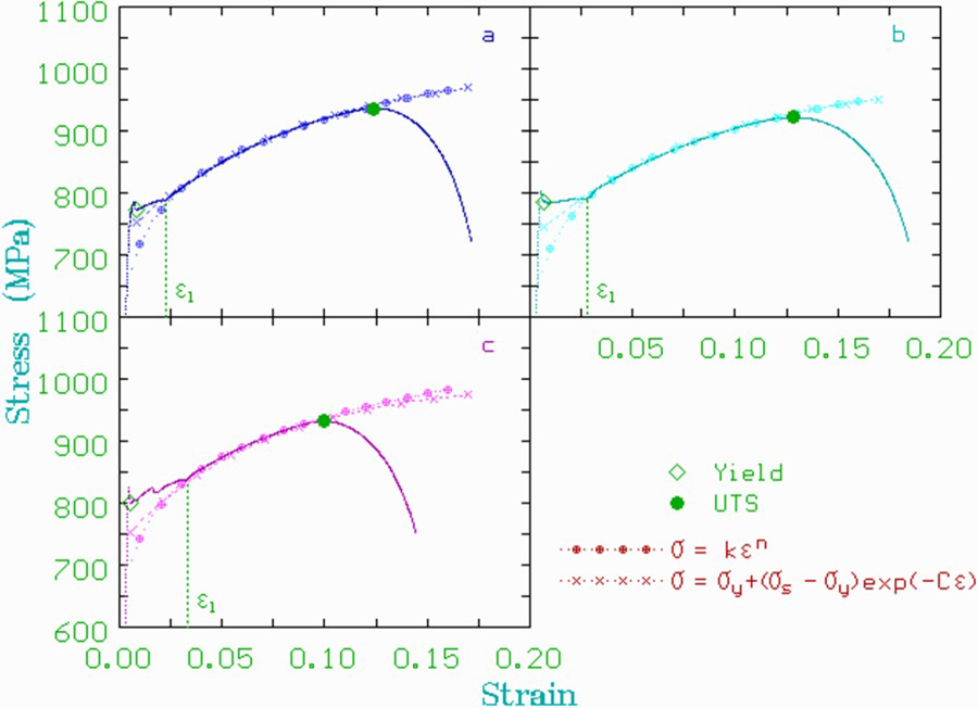
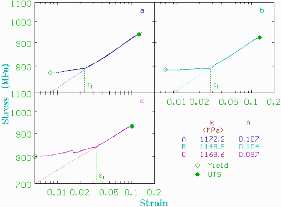
Three tensile samples for each condition were tested, but only one of each was deformed to fracture, as one of them was deformed up to the point of maximum load, which corresponds to the ultimate tensile strength (UTS), and the third specimen was deformed beyond that point but before breaking to analyse the deformation behaviour in the materials. The load-displacement data from the tests were converted into real stress–strain curves by assuming constancy of volume. Figures 5 and 6 shows the stress–strain curves (full lines) for the steels that were tested to fracture for steels A and B, respectively; the curves from samples cut along the three directions (0°, 45° and 90°) were plotted separately in a, b and c graphs, respectively. It should be mentioned that the shape of the stress–strain curves for steel A reflects that of multiphase AHSS, as they do not show an abrupt yield point phenomenon and exhibit a high strengthening rate after yielding, whereas the shape of steel B resembles that of a high-strength low alloy (HSLA) steel in the sense that they exhibit the yield point or Lüders phenomenon and a lower strengthening rate towards the early stages of plastic deformation [3,4].

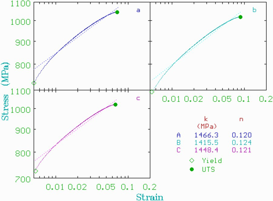
Each curve was fit to equations of the power type proposed by Hollomon [28]: (1) where σ is the stress, ε the strain, and n and k are the straining exponent and coefficient that are obtained by fitting the plastic deformation region, Figures 7 and 8. Each experimental curve was also fit to exponential relationship proposed by Voce [29]: (2) where σ_s is the saturation or steady state stress, σ_o the yield strength and C a coefficient determined from the experimental data. The dashed curves adjusted to Equations (1) and (2) are shown together with the experimental ones.

The values of strain and stress corresponding to the yield and UTS for each testing condition are indicated in their corresponding curve; two points are associated to yielding in steel B, Figure 5, due to the Lüders effect that is observed in the stress–strain curves, the first one corresponds to what is called the lower yield point, whereas the second one is plotted where proper homogeneous deformation starts (ε_l ); Lüders effect is associated in carbon steels to the interaction of interstitial atoms and dislocations and is known as strain aging [30,31]. Figures 5 and 6 show the straight lines that are obtained by fitting stress–strain data in a double logarithm plot to obtain the parameters of Equation (1). The strain domain for these adjustments was that from yielding to UTS in the case of steel A and from the start of homogeneous deformation (ε_l ) to UTS in the case of steel B.

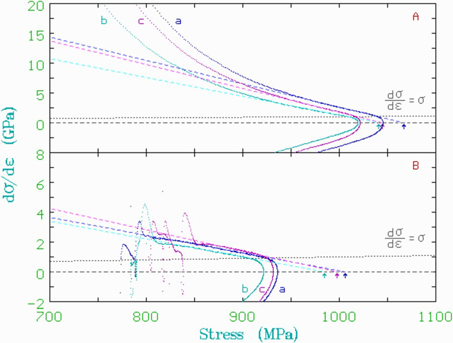
The value of the hardening rate (dσ/dε) is plotted as a function of the stress for each experimental condition, Figure 9. This relationship yields to curves that exhibit a continuous decrease in hardening rate as the stress increases; a straight line in the dσ/dε – σ relationship was adjusted as the curve approaches Considère's criterion expressed by dσ/dε = σ [31]. The slope of this straight line is equal to parameter C in Equation (2), the strength at which dσ/dε = 0 is the saturation stress σ_s , which is indicated by small arrows in Figure 9.

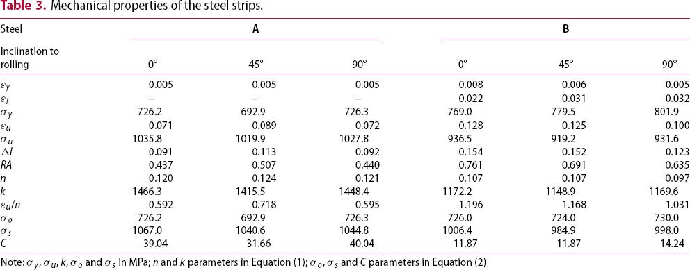
The values for yield stress (σ_y ), ultimate tensile strength (σ_u ), uniform elongation strain (ε_u ), strain to the end of Lüders effect (ε_l , only for steel B), elongation (Δl) and reduction in area (RA) to fracture, as well as those for n, k, σ_o , σ_s , and C are shown in Table 3. It should be mentioned that n and ε_u should be equal for a material that fulfils Hollomon's equation (1), in agreement with Considère's criterion [32].

Discussion

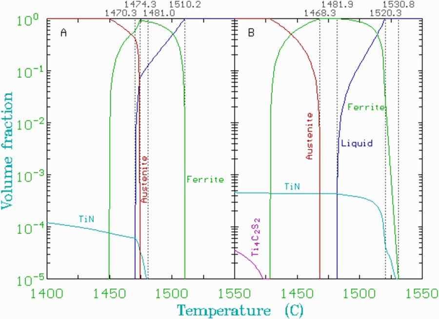
It was mentioned in the preceding section that the chemical composition in both steels differs to achieve the required characteristics, although the carbon content is kept well below that of the peritectic reaction [24,25], Table 1. Steel A contains higher amounts of Cr and Mo to enhance the transformation of austenite into bainite and martensite on cooling. Ti is added to Steel B to promote the formation of TiN; the amount of both elements is such that will promote precipitation of TiN in the melt before the formation of δ-ferrite. Figure 10 shows the transformations that would occur during solidification due to the chemistry of the steels. These transformations were predicted by a thermodynamic and kinetics-based software [20]; the simulation was ended at 1400°C. The critical temperatures for the reactions taking place during solidification are summarised in Table 4.

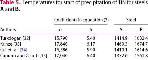
Start of precipitation of TiN was predicted at 1481.0 and 1530.8°C for steels A and B, respectively, which fall within the range computed from the solubility products given by equations of the type: (3) where the amounts of [N] and [Ti] are expressed in mass per cent, T is the absolute temperature and α and β are equilibrium coefficients. Table 5 shows the temperatures calculated from the chemical composition of the steel using the coefficients reported by different authors [33-36].

OPEN IN VIEWER

Figure 4

SE images of samples of steels A and B at their centre (C) and close to the surface (S) together with EDX area analyses that show the absence of central segregation.

OPEN IN VIEWER

Figure 5

Stress–strain curves from samples from steel A cut and tested at 0 (a), 45 (b) and 90° (c) with respect to the rolling direction (full lines); the dotted curves correspond to their fitting to equations (1) and (2).

OPEN IN VIEWER

Figure 6

Stress–strain curves from samples from steel B cut and tested at 0 (a), 45 (b) and 90° (c) with respect to the rolling direction (full lines); the dotted curves correspond to their fitting to equations (1) and (2). The end of Lüders strain is indicated as ε_l .

OPEN IN VIEWER

Figure 7

Double logarithm plot of the stress–strain values to obtain the n and k parameters of equation (1) for steel A.

OPEN IN VIEWER

Figure 8

Double logarithm plot of the stress–strain values to obtain the n and k parameters of equation (1) for steel B. The end of Lüders strain is indicated as ε_l .

OPEN IN VIEWER

Figure 9

Plot of the hardening rate (dσ/dε) as a function of stress for steels A and B. The straight line fitted to the experimental data allows for determining σ_s , and C.

OPEN IN VIEWER

Table 3

Mechanical properties of the steel strips.

Steel	A			B
Inclination to rolling	0°	45°	90°	0°	45°	90°
εy	0.005	0.005	0.005	0.008	0.006	0.005
εl	–	–	–	0.022	0.031	0.032
σy	726.2	692.9	726.3	769.0	779.5	801.9
εu	0.071	0.089	0.072	0.128	0.125	0.100
σu	1035.8	1019.9	1027.8	936.5	919.2	931.6
Δl	0.091	0.113	0.092	0.154	0.152	0.123
RA	0.437	0.507	0.440	0.761	0.691	0.635
n	0.120	0.124	0.121	0.107	0.107	0.097
k	1466.3	1415.5	1448.4	1172.2	1148.9	1169.6
εu /n	0.592	0.718	0.595	1.196	1.168	1.031
σo	726.2	692.9	726.3	726.0	724.0	730.0
σs	1067.0	1040.6	1044.8	1006.4	984.9	998.0
C	39.04	31.66	40.04	11.87	11.87	14.24

Note: σ_y , σ_u , k, σ_o and σ_s in MPa; n and k parameters in Equation (1); σ_o , σ_s and C parameters in Equation (2)

OPEN IN VIEWER

Figure 10

Solidification reactions for A and B steels as predicted by the thermodynamic and kinetics-based software.

OPEN IN VIEWER

Table 4

Solidification reactions taken place in the steels.

	A				B
Constituent	T (C)	Vf	T (C)	Vf	T (C)	Vf	T (C)	Vf
Liquid	1510.2	1	1470.3	0	1530.8	1	1482.4	0
δ ferrite	1510.2	0	1485.4	1	1520.3	0	1481.9	1
δ ferrite	1474.3	1	1427.1	0	1468.3	1	1428.8	0
Austenite	1474.3	0	1400.0	1	1468.3	0	1400.0	1
TiN	1481.0	0	1400.0	1.21·10−3	1530.8	0	1400.0	4.56·10−3

OPEN IN VIEWER

Table 5

Temperatures for start of precipitation of TiN for steels A and B.

	Coefficients in Equqation (3)		Steel
Authors	α	β	A	B
Turkdogan [32]	15,790	5.40	1414.9	1632.4
Kunze [33]	17,640	6.17	1469.3	1674.7
Cui et al. [34]	16,586	5.90	1410.1	1614.6
Capurro and Cicutti [35]	17,040	6.40	1372.6	1561.8

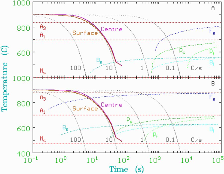
The transformation of the strips during the run-out table cooling was simulated with the aid of the software mentioned above [20] feeding their compositions. The software predicts the temperatures at which transformation to ferrite, pearlite and bainite start as a function of the cooling rate, identified as F_s , P_s and B_s , respectively, and at which the transformation to pearlite and bainite finish, P_f and B_f , respectively. The CCT diagrams for both compositions are shown in Figure 11. The critical temperatures (A₁ , A₃ and M_s ) are shown in this figure and in Table 5. The greater content in alloying elements in steel A promotes the shifts of curves corresponding to F_s , P_s , B_s , P_f and B_f to higher times and would result in delaying the occurrence of such microstructures. The CCT diagram was calculated using a finish rolling temperature of 900°C and an austenite grain size of 20 µm, which were the values predicted by modelling hot rolling of steel [16,21,22]. The cooling curves at the surface and centre of a 3.6 mm strip are shown in Figure 11. These curves were obtained from a heat transfer model developed to compute the temperature distribution within steel strips that are being cooled within a run-out table [17]; the cooling time in the run-out table was set as 30 s; coiling was predicted to occur at 593°C. These results confirm the microscopical observations shown in Figures 1–3 and in Table 2 in the sense that both steels will transform into a mixed microstructure made of ferrite, bainite and martensite; the highest alloying content of steel A will result in a higher amount of martensite in comparison with steel B, as it is presented in Table 2. No pearlite was found in the micrographs, and this may be due to the low carbon content of the steels (0.065 and 0.056, respectively, for steels A and B), Table 1.

OPEN IN VIEWER

Figure 11

Continuous cooling transformation for steels A and B and the computed temperatures at the centre and surface of the strip using the model described elsewhere [16].

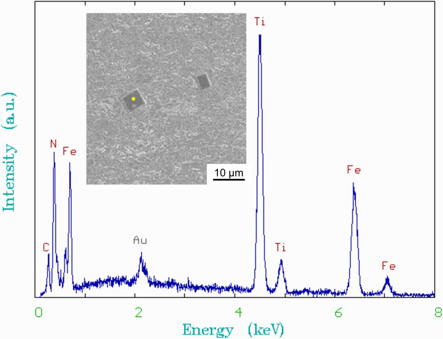
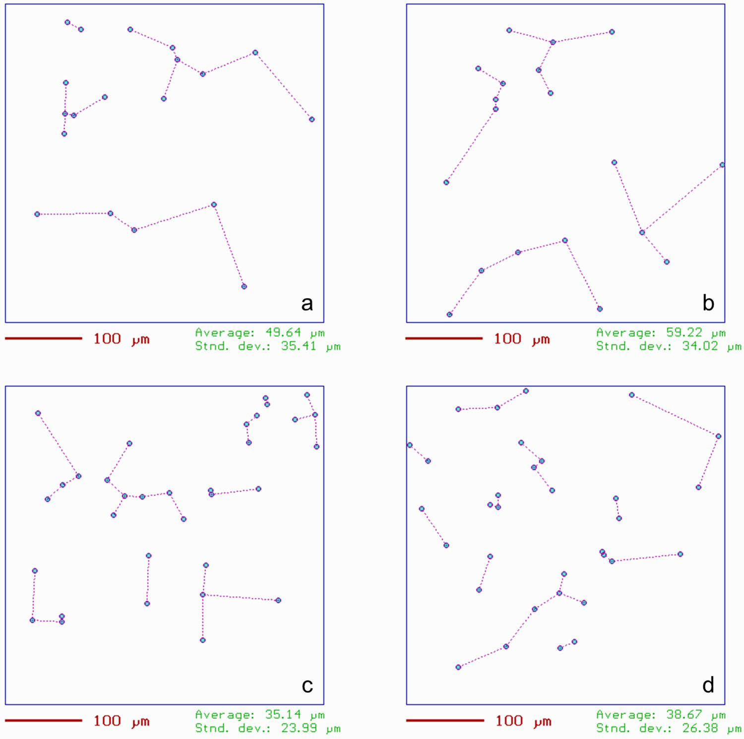
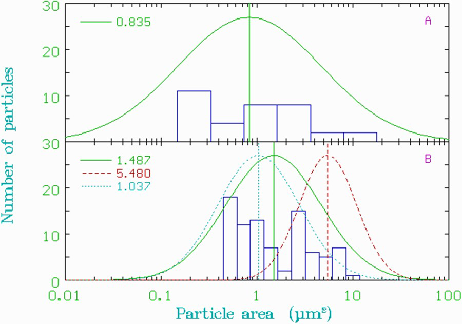
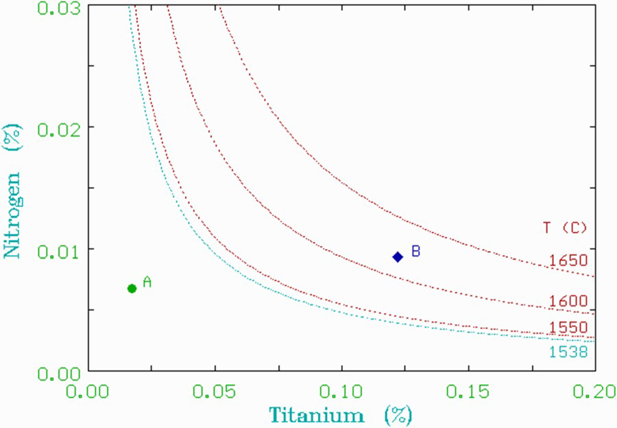
It was pointed out in Figure 1 the presence of a coarse particle towards the centre of steel B; EDX analyses conducted in such particles revealed that they are made of TiN, Figure 12. Extensive observations by SEM were carried out in both steels in locations close to their centres and surfaces to record the size of distribution of such particles. The distances between the TiN particles were analysed by recording their coordinates from SEM micrographs and calculating the distance between close neighbours following the procedure described elsewhere [37]. Figure 13 shows that the distance between precipitates is smaller in samples from steel B, as may be expected from the smaller volume fraction obtained from the solidification analyses, Table 5; it was observed that the distances between closer neighbours was smaller towards the centre of the strip, and this may be due to the lower solidification rates occurring towards the centre of the slab [35], which allow for the alloying elements to segregate. The size of the TiN precipitates was characterised by their area, and it was analysed their distribution assuming it to follow a log-normal scale. The results shown in Figure 14 indicate that the particles in steel A follow a single distribution, whereas those from steel B follow a bimodal distribution, therefore the average of the whole population and of the bigger and smaller distributions are shown; what is of interest is that the average area size of the precipitates in steel A is close to the size of the smaller population of steel B. Such behaviour may be explained by observing Figure 15, where the temperatures predicted for the precipitation of TiN particles using Equation (3) with the coefficients from Turkdogan [33] are shown as a function of the chemical composition of the steels. It can be appreciated that the chemical composition of steel B will allow for precipitation to take place while the steel is liquid and the particles will be able to grow, therefore the bigger size population. Precipitation of TiN will proceed in steel A at a lower temperature, as well as in steel B, therefore the similarity in size of the smaller precipitates, which are sought after to enhance the mechanical properties of the steels [12,27,35].

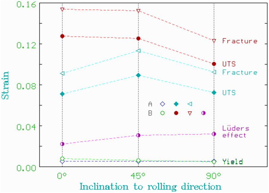
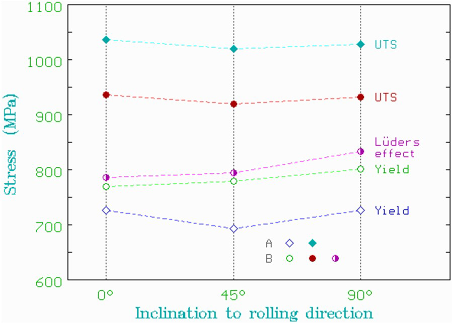
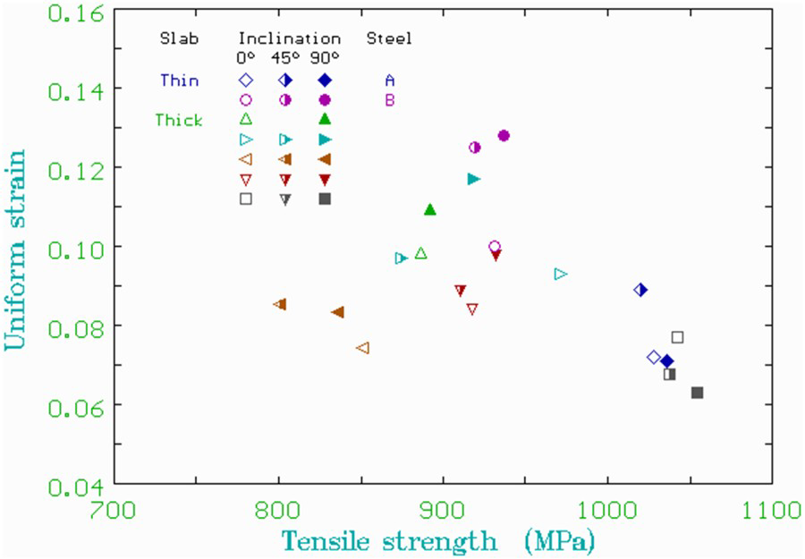
Figures 16 and 17 show, respectively, the properties associated to strain and stress, respectively, from the tensile tests in both steels. It is appreciated that steel A is more ductile when the sample is cut at 45° to the rolling direction, but this does not hold for steel B as the sample tested along the rolling direction results to be more ductile, Figure 16. The occurrence of a Lüders type effect taking place in steel B was stated when Figures 6 and 9 were first mentioned, and the contribution of such effect is significant in terms of the total strain that the material sustains, the strain involved in such effect may be detrimental to the total straining, as it is shown for the samples tested in the transverse direction to rolling (90°). Figure 17 shows that yielding occurs at a lower stress in steel A in comparison to the other material, but its strengthening to the UTS value is much higher. Figure 18 compares the values of the strain and stress to the point of maximum load of the steels studied in this work (A and B) with unpublished results of steel samples obtained from sheets obtained from conventional, thick, slabs, it can be appreciated that the data points follow a similar behaviour.

Figures 5 and 6 show the experimental stress–strain curves for both steels and their fitting to constitutive equations of the power and exponential type. Figure 5 shows that fitting the data to power relationship, Equation (1), does only agree within a short strain domain, whereas that to exponential type (2) agrees over the yielding to UTS straining domain. Moreover, Equation (2) has been justified in terms of the changes that take over dislocation arrangement as a result of the equilibrium between the dislocations being created to sustain the plastic deformation and their annihilation by restoration mechanisms [38-40] and has been used in analyses of plastic deformation in complex multiphase steels [41-43]. Use of power type of equation (1) has been criticised by their limitations in covering the full range of plastic strain and that they predict infinite strength [44]. In some cases, the stress–strain curve has been fitted into various segments, each with different values for parameters k and n [45,46]. Figure 6 shows that both types of equations fit with accuracy the experimental data once the Lüders strain has been surpassed. The proximity of the values of exponent n and that for the strain to the UTS in this steel confirm the fitting of this material to power type equations. In all cases, the fittings to either equation between the yield point and the end of Lüders strain are underestimated. The biggest divergence occurs in the case of Equation (2), as parameter σ_o is lower than the yield strength (σ_y ), Table 3. Such difference may point to the strengthening that results in steel B due to the amount of nitrogen and carbon in solution, rather than combined with titanium or other alloying elements.

Conclusions

The steels that were studied were designed to fulfil the requirements demanded by AHSS, as both are made of multiple microstructural constituents such as ferrite, bainite and martensite. Both steels were made by the thin slab casting and direct hot-rolling route and had limited amounts of carbon, the rate of solidification of the casting process suppresses the segregation at the centre of the slab. Steel A relied on the increase of alloying elements that would retard the transformation of the steel into ferrite while cooling in the run-out table; steel B has also alloyed with elements that contribute to retarding the transformation to ferrite, but with limited contents. The results obtained show a similar trend observed in samples obtained from conventional cast steels.

OPEN IN VIEWER

Figure 12

EDX spectrum of a TiN particle found towards the centre of strip B.

OPEN IN VIEWER

Figure 13

TiN precipitates in samples from steels A (a and b) and B (c and d) close to the centre (a and c) or surface (b and d) of the strips. The straight lines connect the closest neighbours.

OPEN IN VIEWER

Figure 14

Particle area distribution of TiN precipitates found in steels A and B.

OPEN IN VIEWER

Figure 15

Temperatures for the precipitation of TiN as a function of their contents as calculated with the coefficients proposed by Turkdogan [31]. The points corresponding to steels A and B are shown. The solidification temperature of 1538° for iron is indicated [23].

OPEN IN VIEWER

Figure 16

Changes in properties related to the strain in both steels in different testing directions.

OPEN IN VIEWER

Figure 17

Changes in properties related to the strength in both steels in different testing directions.

OPEN IN VIEWER

Figure 18

Comparison of the values of strain and stress to the point in maximum load obtained from samples obtained from casting in thin and thick slabs.

Both steels had added Ti and N to promote the precipitation of TiN particles to increase their strength, but the higher amounts of both in steel B may promote their precipitation in the liquid state before that that would take place during hot-rolling or even during cooling in the run-out table. As a result of this, TiN area size distribution in steel B shows to be bimodal.

The experimental stress–strain curves were fitted to equations of the power and exponential type. The exponential equation was found to reproduce the curves of steel A. The plastic behaviour of steel B was found to be well fitted by either type of curve, but the strength was underestimated by both equations in the Lüders band region.