Sulphide capacity prediction of CaO–SiO 2 –MgO–Al 2 O 3 slag system by using regularized extreme learning machine

Abstract

Desulphurization is essential in the steelmaking process for high-quality steel production, and sulphide capacity has proven to be an effective index to evaluate the desulphurization ability of molten slag or flux. Several analytical or empirical models have been proposed to calculate the sulphide capacity. However, these models usually show insufficient generalization ability when new variables/data are introduced, which limits their practical application. In this work, experimental data were collected from the literature and a regularized extreme learning machine (RELM) model was established to predict the sulphide capacity of the CaO–SiO₂–MgO–Al₂O₃ slag system. The results demonstrated that the proposed model is robust for the prediction of sulphide capacity under different conditions. The coefficient of determination (R ²), correlation coefficient (r), root-mean-square error (RMSE) of the optimal model reached 0.9763, 0.9881, 0.113, respectively, which outperform the results of the reported models.

1. Introduction

The demand for sulphur control is becoming increasingly stringent in molten steel to produce high-quality steel. A much more reliable slagging regime is also highly required in the desulphurization process due to the deteriorating ore quality [1–4]. The sulphide capacity (Cs) proposed by Richardson et al. [5], was a well-recognized index to evaluate the desulphurization ability of slag in the steelmaking and has attracted great attention to quantify the value of Cs under various conditions, such as temperature and basicity.

There are currently three strategies to calculate or predict the Cs in the literature. One is to develop empirical models and then obtain the correlation between Cs and other parameters, including composition of slag, optical basicity and processing temperature etc. [6]. Some typical models were proposed by Sosinsky et al. [7], Young et al. [8] and Zhang et al. [9]. The calculation results of these models are in good agreement with experimental results, but only within a limited range of composition and temperature. Once the values of these parameters exceeded the boundaries of the certain composition and temperature, the obtained calculate deviation with the high value resulted in the developed model fail for practical application. The second strategy based on the principle of Short Range Order (SRO) has been incorporated into some commercial software packages, such as FactSage© and ThermoSlag to calculate the Cs [10–12] under a large range of conditions. FactSage© is a multi-module software for thermodynamic simulation, which is well suited for calculating thermodynamic data with visualized diagram or figure, such as phase diagrams, phase equilibria, E-pH diagrams, heat balances, etc. However, the calculation process is complicated when the Cs is calculated [1]. ThermoSlag is a software developed based on KTH model for predicting the thermodynamics and thermophysical properties of slag. However, too many parameters need to be optimized in KTH model [9]. The third strategy is based on the burgeoning intelligent algorithm to establish the nonlinear correlation between Cs and other parameters, and this approach has gained a growing interest in metallurgical research field due to its features of simple operation and high precision. Recently, Derin et al. [13] predicted the sulphide capacity in the binary and multi-component melts system under various temperatures using a neural network approach. The calculated results matched well with the experimental results. Ma et al. [1] used an Artificial Neural Network (ANN) to predict the sulphide capacity and achieved promising performance by comparing with the known empirical models.

Another widely used algorithm is extreme learning machine (ELM), which has been proposed for training single hidden layer feedforward neural networks (SLFNs). The ELM has two main advantages [14,15]: (1) The connection weight between the input and the hidden layers and the threshold value of the hidden layers are randomly generated in the ELM algorithm, and the unique optimal solution is obtained quickly by setting the neuron number of the hidden layers. This arrangement can avoid the repeated adjustment of connection weight and threshold value in the conventional neural network. (2) The connection weight (β) between the hidden layer and the output layer can be determined by solving a system of equations. This solution could allow better generalization ability and higher calculation efficiency than that from the principle of the iterative algorithms, such as ANN. For instance, Chen et al. [16] applied the ELM model to predict the quality of continuous-casting billets, showing the prediction accuracy of ELM model is the highest by comparing with the back propagation (BP) neural network model and the BP neural network model improved by genetic algorithm. Guan et al. [17] used the intelligent algorithm combining ELM and the algorithm of image processing in image classification indicating superior to the conventional intelligent classification method by comparing label consistency, detail preservation, and computational speed. Zou et al. [18] applied the regularized extreme learning machine (RELM) model to predict the carbon segregation index of continuous-casting billets, showing the prediction accuracy of RELM model is the highest by comparing with the multiple linear regression model and the ELM model. However, to the best of our knowledge, few efforts have been made to use the ELM algorithm for the prediction of the Cs value.

In this work, an attempt has been made to develop a modified ELM to predict Cs in a popularly used desulphurization slag system under different conditions. According to experimental data that collected from the previous studies, the correlation was established between the input and output variables. The novel RELM model was concretely utilized to predict the Cs in CaO–SiO₂–MgO–Al₂O₃ slag system and its performance was evaluated by using different statistical evaluation indexes. It is expected to build a more reliable and efficient mathematical model to calculate the Cs so as to promote high-efficiency desulphurization in the steelmaking process.

2. Cs calculation using RELM model

2.1. Analysing of database and data

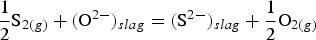
The principal equilibrium reaction in the process of desulphurization between slag and gas is expressed as follows:

(1)

The equilibrium constant (K) of Reaction (1) is displayed as: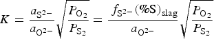 (2) where represents the activity of ionic sulphur in slag; is the activity of ionic oxygen in slag; denotes the activity coefficient of ionic sulphur in slag; (%S)_slag is the weight per cent of sulphur content in slag; the indicates the partial pressure of oxygen gas; the means the partial pressure of sulphur gas.

The mean sulphide capacity (Cs) works as a function of temperature and slag composition, and the definition of Cs is expressed by Richardson et al. [5] using Equation (3):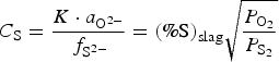 (3)

The experimental data came from the lab experiments and are summarized in Table 1. There are 298 groups of data in total and they are comparable, as the data were obtained based on the classical gas-slag equilibrium theories and techniques. Meanwhile, in the present study, the equilibrium times of the collected data were at least 4 h for the slag and gas mixture to reach theoretical equilibrium at the experimental temperature in order to assure consistent and comparable results [5,19–29]. In addition, these data were also used by other researchers to predict Cs using various models, such as ANN [1]. According to the definition of Cs, some variables that related to the Cs calculation were used as the input parameters, which were the chemical compositions of the CaO–SiO₂–MgO–Al₂O₃ slag system and other conditions, including (wt-%CaO), (wt-%SiO₂), (wt-%MgO), (wt-%Al₂O₃), (wt-%S)_slag, temperature, and . All the previous studies had measured and .
Table 1.
Experimental data used for the RELM prediction of Cs.

Slag System Number Ref.

CaO–Al₂O₃ 5 [5,21]

CaO–SiO₂–Al₂O₃ 71 [20,21,23,24,28]

CaO–MgO–Al₂O₃ 40 [21,24]

CaO–SiO₂–MgO–Al₂O₃ 182 [19,21–23,25–29]

A scatter diagram and a Pearson correlation coefficient were used to determine the relationship between these parameters. The scatter matrix visualization of the data sets was performed using the Pandas Module and the Matplotlib Module in the Python language calculating program, as shown in Figure 1. In Figure 1, the histograms on the diagonal of the figure show the data distribution of a single variable, and the scatter plots on the upper and lower triangles show the relationship between two variables. For instance, the left-most graph in the bottom row of Figure 1 shows the relationship between the temperature and the logarithm of Cs (LogCs). The value of temperature ranged from 1313 to 1928K. The range of the weight per cent for CaO, SiO₂, MgO, and Al₂O₃ was 6.77–68.02, 0–84.50, 0–23.10, and 7–61.72 wt-%, respectively. The range of the weight per cent for sulphur content in slag was from 2.94 × 10⁻⁴ to 2.70 wt-%. The value of ranged from 2.70 × 10⁻⁴ to 5.23 × 10⁻² and the value of Log C_S ranged from −5.74 to −1.71.
Figure 1.
Scatter plot matrix visualization of (wt-%CaO), (wt-%SiO₂), (wt-%MgO), (wt-%Al₂O₃), (wt-%S)_slag, temperature, and Log Cs.

Figure 2 shows the correlation between input variables and output variables that analysed using the Numpy Module and the Matplotlib Module of the Python program. In Figure 2, the radial distance represents the value of the correlation coefficient between Log C_S and temperature, (wt-%CaO), (wt-%SiO₂), (wt-%MgO), (wt-%Al₂O₃), (wt-%S)_slag, , respectively. The calculation principle of correlation was mainly based on the formula of the Pearson correlation coefficient in the statistics analysis, as shown in Equation (4). In Figure 2, the different impacts of input variables on Log C_S are shown in an order from strong to weak as: (wt-%SiO₂), (wt-%CaO), (wt-%Al₂O₃), (wt-%S)_slag, , temperature and (wt-%MgO). (4) where is the mean of variable x; is the mean of variable y; x_i is the ith value of variable x; y_i is the ith value of variable y.
Figure 2.
Correlation analysis results between input variables and output variables.

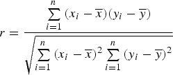
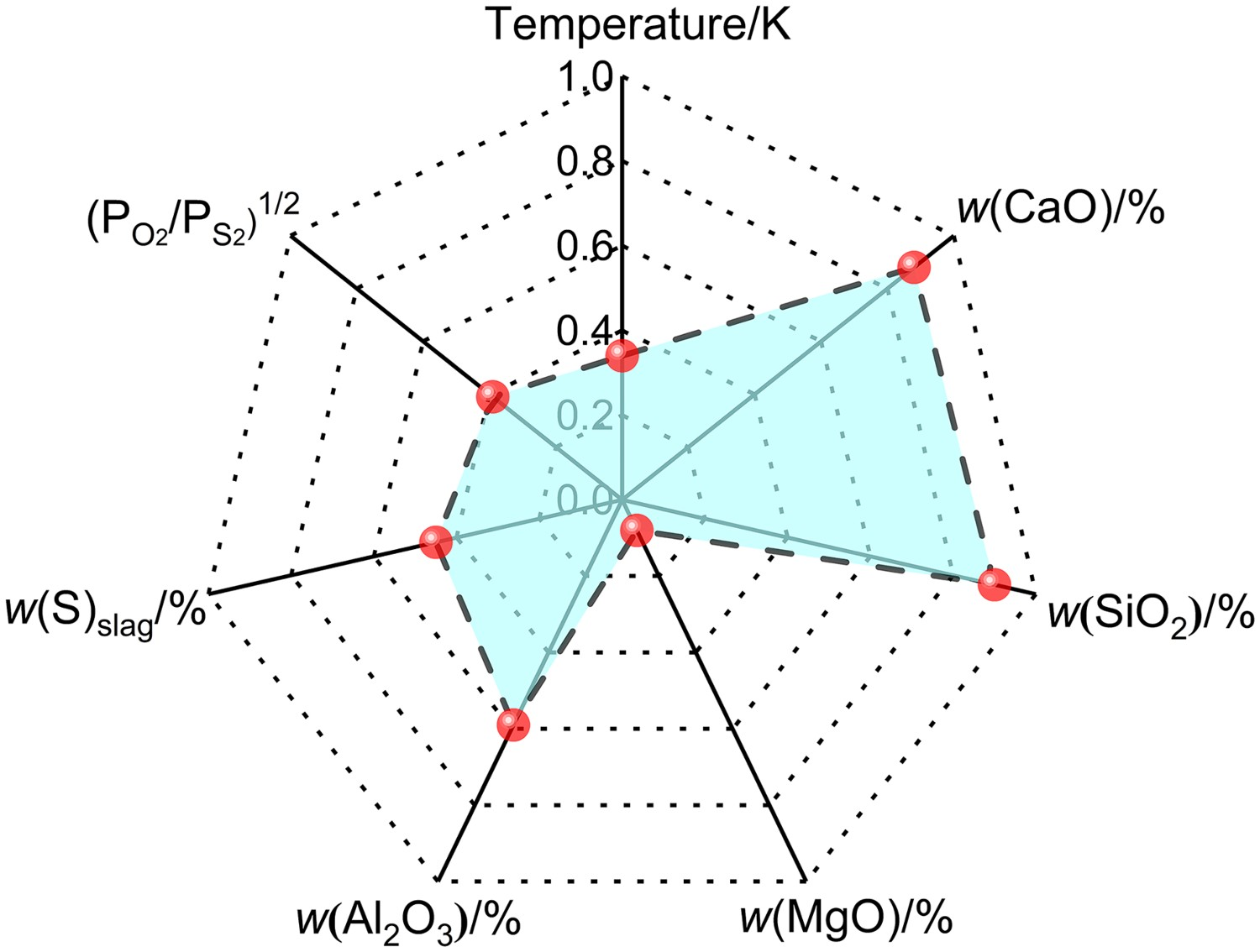
In the right-bottom of Figure 2, the value of Pearson correlation coefficient between the Cs and (wt-%MgO) was 0.08, indicating the Cs weakly correlated with the composition of (wt-%MgO) in this CaO–SiO₂–MgO–Al₂O₃ slag system. Subsequently, the significance of correlation coefficient was tested by using the Student’s t-Test, as shown in Eq. (5). When the P-value of significance probability is less than 0.05, it means that the correlation of variables is significant. When the P-value is less than 0.01, it means that the correlation of variables was very significant. When the P-value is greater than 0.05, it means that the correlation of variables is not significant [30].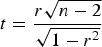 (5) where r is the correlation coefficient; n is the sample size of variable; n − 2 is the degree of freedom.

Table 2 shows the calculation results of correlation analysis based on the formula in Eq. (5). The P-value is less than 0.01 between Log C_S and temperature, (wt-%CaO), (wt-%SiO₂), (wt-%Al₂O₃), (wt-%S)_slag, , respectively. However, the P-value is 0.173 between Log C_S and (wt-%MgO). Taken together, these results indicated that the relationship between temperature, (wt-%CaO), (wt-%SiO₂), (wt-%Al₂O₃), (wt-%S)_slag, and Log C_S reach very significant correlation. However, there is no significant correlation between Log C_S and (wt-%MgO).
Table 2.
The calculation results of P-value between Log Cs and input parameters.

P-value T (wt-%CaO) (wt-%SiO₂) (wt-%MgO) (wt-%Al₂O₃) (wt-%S)_slag

Log Cs 0.000 0.000 0.000 0.173 0.000 0.000 0.000

2.2. Modelling in RELM

Slag System	Number	Ref.
CaO–Al₂O₃	5	[5,21]
CaO–SiO₂–Al₂O₃	71	[20,21,23,24,28]
CaO–MgO–Al₂O₃	40	[21,24]
CaO–SiO₂–MgO–Al₂O₃	182	[19,21–23,25–29]

P-value	T	(wt-%CaO)	(wt-%SiO₂)	(wt-%MgO)	(wt-%Al₂O₃)	(wt-%S)_slag
Log Cs	0.000	0.000	0.000	0.173	0.000	0.000	0.000

In the conventional neural network, the connection weight (β) between the hidden layer and the output layer is determined by using multiple iterations, which causes slow convergence rate of the network and even falls into local minimum easily. Therefore, Huang et al. [15,31] proposed a novel neural network – ELM, which exhibited fast computation speed compared with the traditional BP neural network.

Figure 3 shows the structure diagram of ELM networks with the three layers, including the input layer, the hidden layer and the output layer. Normally, the ELM model is constructed based on the least squares loss function in the statistics. In the ELM model, only the empirical risk is considered to minimize without the consideration of structural risk, which may lead to over-fitting of the model. In order to establish an excellent model, both empirical risk and structural risk should be considered in the ELM model. Therefore, for the sake of further improving the generalization ability of the conventional ELM, the regularization coefficient used for adjusting the proportion of empirical risk and structural risk was introduced to establish the RELM models [32].

Figure 3.

Structure diagram of ELM networks.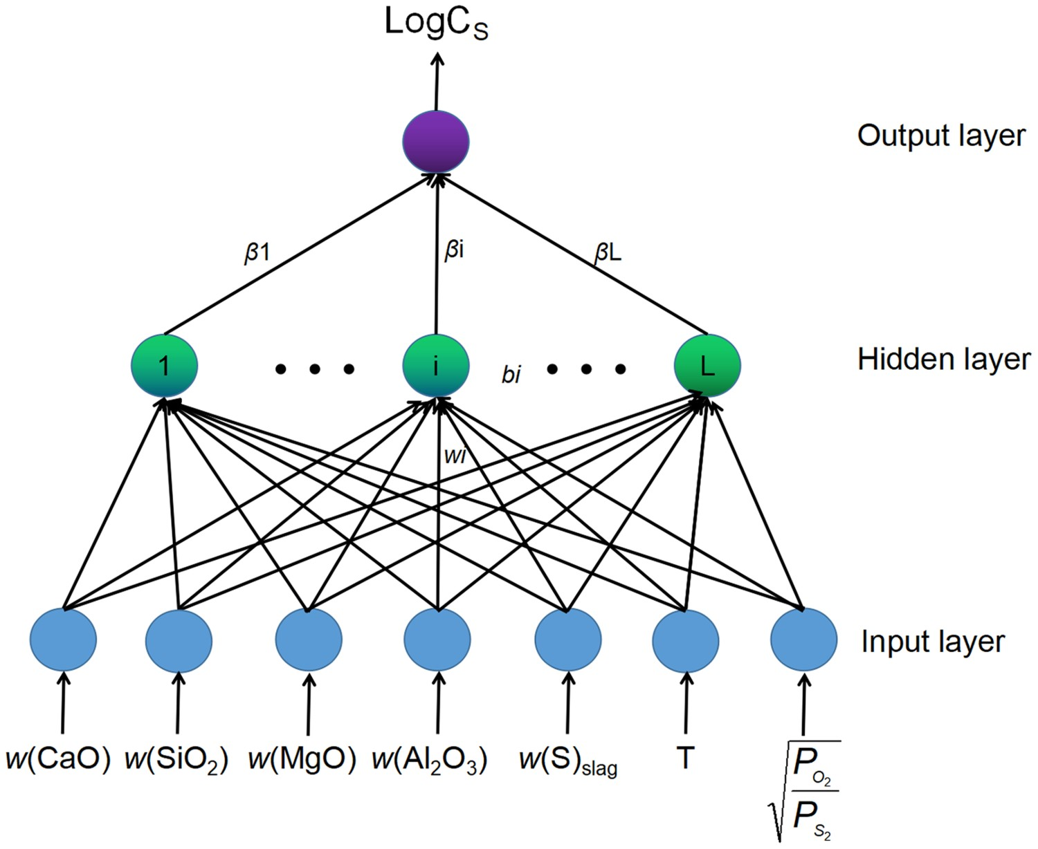

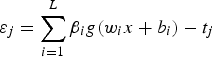
The output function of the ELM model can be expressed by Equation (6):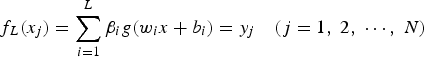 (6) where L is the number of hidden layers; g(w_ix + b_i ) is the activation function; w_i is the matrix of the input weights; β_i is the matrix of the output weights; b_i is the offset value of the hidden layer; x is the input dataset of the ELM network; y_j is the output dataset of the ELM network.

The objective function of the ELM network is shown in Equation (7):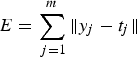 (7) where y_j is the output vector of the Cs and t_j is the output vector of the ELM network training.

The minimum of the objective function can be obtained to calculate w_i , β_i , b_i in this case. The introduction of the regularization coefficient can significantly enhance the generalization ability of the ELM approach by adjusting the proportion of empirical risk and structural risk. The RELM model can, therefore, be summarized in the following four sections:

(1) The objective function of the RELM model is shown in Equations (8) and (9):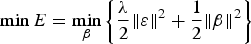 (8) (9) where λ is the regularization coefficient; ||ε||² is the empirical risk; ||β||² is the structural risk; ε_j is the training error; t_j is the output set.

(2) The Lagrangian function is constructed as shown in Equation (10):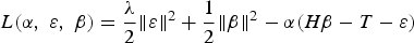 (10) where α = [α ₁, α ₂, α ₃, α_m ] is the Lagrangian operator; H is the output matrix of hidden layer; T is the desired output matrix.

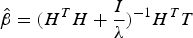
(3) The can be obtained when the partial derivatives be zero for each variable of the Lagrangian function, as shown in Equation (11). (11) where I is the unit matrix and is the solution of .

(4) The prediction model of the RELM obtained when combining Equation (11) and Equation (6) can be expressed as Equation (12).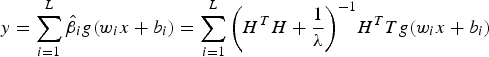 (12)

In this study, the 298 groups of experimental data were divided into two categories, of which the 198 groups were used to train the model, and the left 100 groups were used to test the model. The flowchart of the entire process is illustrated in Figure 4. The prediction results of Cs values were calculated under the different input variables and activation functions. As shown in Table 3, shown in Model 1 to Model 3 are the input variables and activation functions, which do not contain (wt-%MgO); Model 4 to Model 6 show the input variables and activation functions, which contain (wt-%MgO). In the RELM model, the main activation functions include Sinusoidal (Sin), Sigmoid (Sig), and Hardlim. The regularization coefficient (λ) was determined according to the hit rate of the error between the calculated value and the experimental value of Log C_S within the range of ±0.3.

Figure 4.

A flowchart of using RELM model to process the data.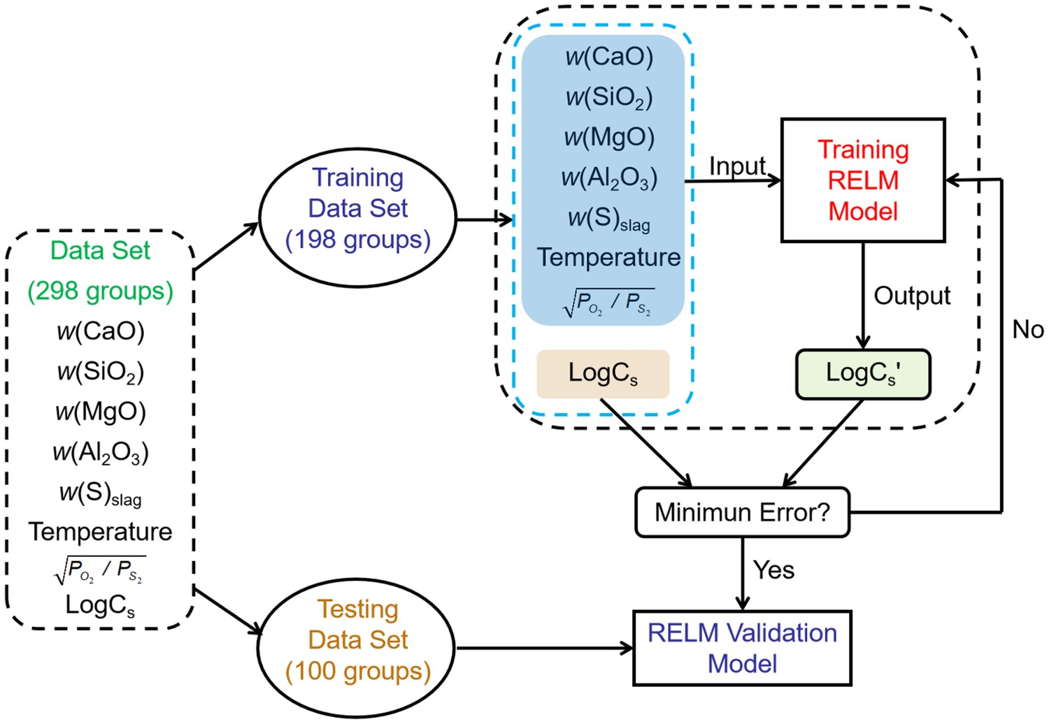

Table 3.

Definition of RELM models 1–6 according to the input variables and activation functions.

	Model1	Model2	Model3	Model4	Model5	Model6
Activation function	Sin	Sig	Hardlim	Sin	Sig	Hardlim
(wt-%CaO)	√	√	√	√	√	√
(wt-%SiO₂)	√	√	√	√	√	√
(wt-%MgO)				√	√	√
(wt-%Al₂O₃)	√	√	√	√	√	√
(wt-%S)_slag	√	√	√	√	√	√
T	√	√	√	√	√	√
	√	√	√	√	√	√

In Figure 5, it has a regularization coefficient and a corresponding hit rate under different activation functions when the error between the Log Cs obtained by using experiments and the Log Cs obtained by using RELM model is within the range of ±0.3. The hit rate of models reaches the maximum when the regularization coefficient is 0.8.

Figure 5.

Regularization coefficient vs. hit rate under conditions of Sinusoidal (Sin), Sigmoid (Sig), and Hardlim.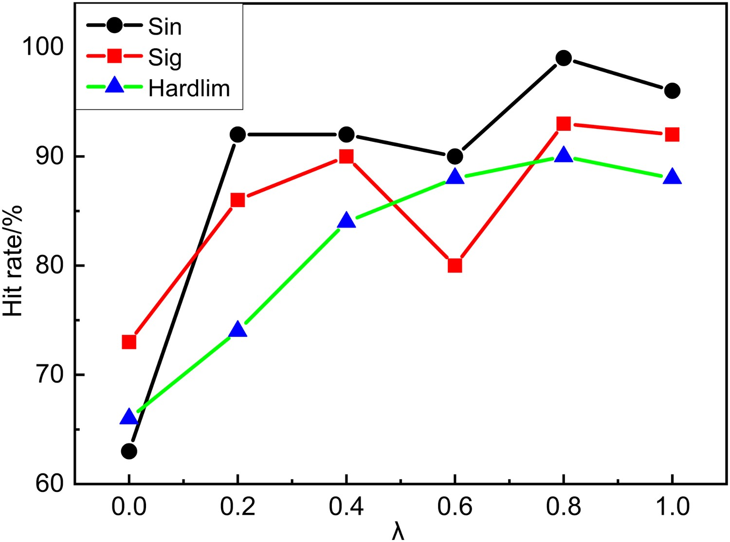

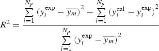
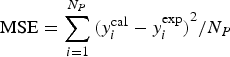
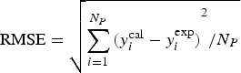
2.3. Model evaluation

The performance of RELM models was evaluated according to different statistical evaluation indexes, including the coefficient of determination (R ²), mean square error (MSE), and root-mean-square error (RMSE). The mathematical definitions of the above indexes are displayed in Equations (13)–(15):

(13) (14) (15) where N_p is the number of the total data set; y is the value of Cs; is the average value of the Cs; the ‘exp’ means the experimental values; the ‘cal’ means the calculated values.
3. Results and discussion

3.1. The effect of MgO and activation function on Cs

The RELM models were established according to Table 3. The prediction results of the models shown in Table 4 demonstrate that the (wt-%MgO) has little effect on the calculation of Cs by using RELM model. To be specific, when the activation functions are the same, the computation speed of Model 4, Model 5, and Model 6 increases 0.006, 0.0054, and 0.0065 s, respectively, after removing the variable of (wt-%MgO). The difference of the RMSE between Model 1 and Model 4 is 0.0114. Plenty of literatures prove that global scholars have different opinions about the effect of MgO on Cs. According to the Sosinsky et al.’s model [7] and the Young et al.’s model [8], it is known that MgO has little effect on the calculation model of Cs. There is a negative correlation between MgO and Cs when the Cs is calculated by using KTH model [11]. However, Taniguchi et al. [22] reported that the Cs increases by the addition of MgO.

Table 4.

Results of various models.

	Model1	Model2	Model3	Model4	Model5	Model6
R ²	0.9712	0.9518	0.9355	0.9763	0.9544	0.9482
r	0.9855	0.9756	0.9672	0.9881	0.9770	0.9738
MSE	0.0158	0.0269	0.0334	0.0131	0.0252	0.0291
RMSE	0.1257	0.1640	0.1827	0.1143	0.1587	0.1707
Time/s	0.0715	0.0701	0.0646	0.0775	0.0755	0.0711

The prediction results shown in Table 4 also indicate that the Model 1 has the best prediction effect, when (wt-%MgO) is not contained and the activation function is ‘Sin’. Besides, the model 4 has the best prediction effect, when (wt-%MgO) is contained and the activation function is ‘Sin’. The comparison results between the prediction value and the experimental value are shown in Figure 6. The dashed lines in these figures indicate the ideal line of Cs (prediction value = experimental value) as with Figure 6. In Figure 6, it can be seen that the hit rate from Model 1 to Model 3 is 99%, 93%, and 88%, respectively, when the variable of (wt-%MgO) is not included and the error between the Log Cs obtained by using experiments and the Log Cs obtained by using RELM model within the range of ±0.3; the hit rate from Model 4 to Model 6 is 99%, 93%, and 90%, respectively, when the variable of (wt-%MgO) is included and the error within the range of ±0.3. In summary, Model 1 and Model 4 are closer to ideal state than other models, and the activation function of sinusoidal shows better performance in the RELM models.

Figure 6.

Comparison between experimental and calculated Cs values obtained by (a) Model 1, (b) Model 2, (c) Model 3, (d) Model 4, (e) Model 5, and (f) Model 6.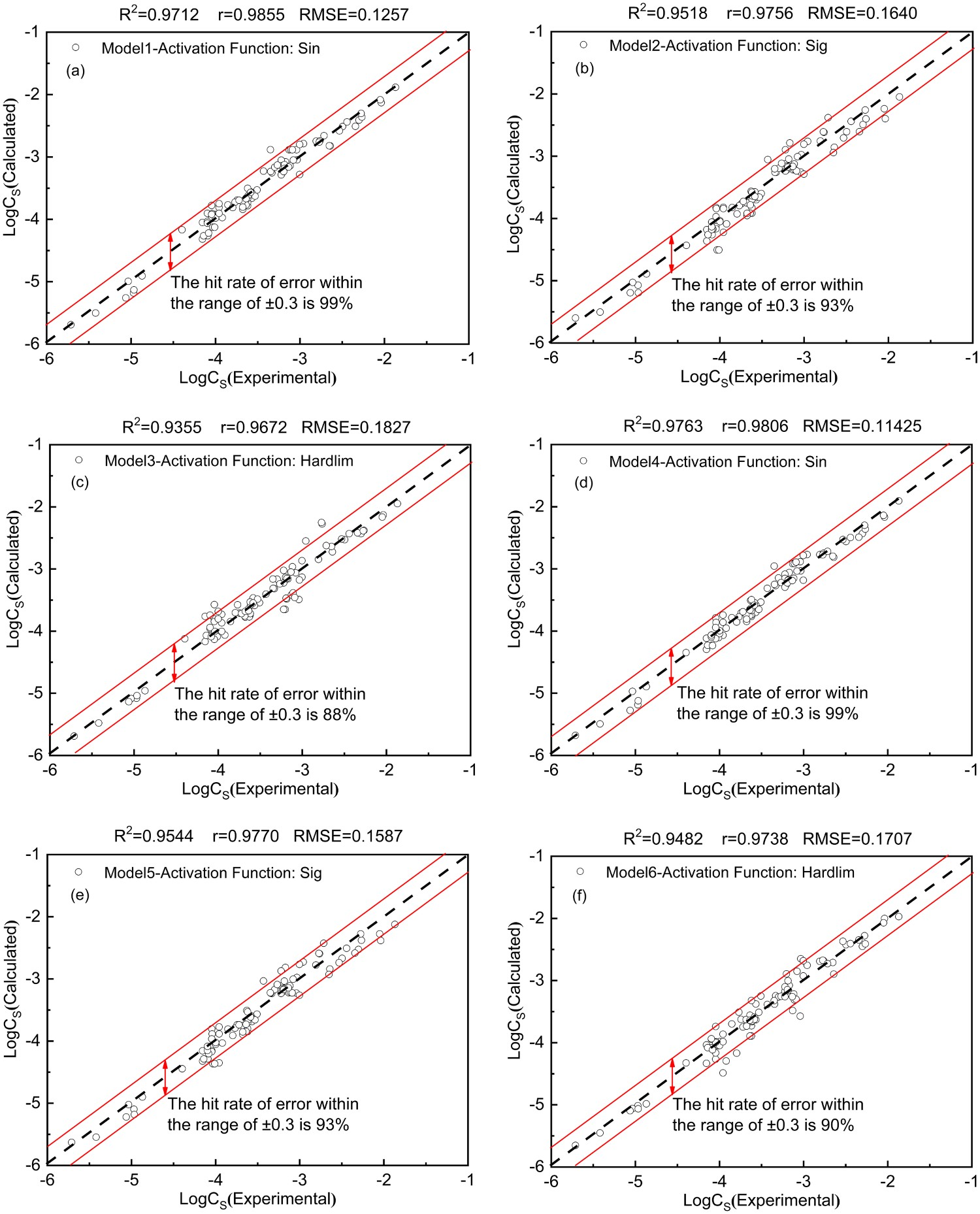

3.2. Comparison of the RELM model with other models

In order to verify the accuracy of the RELM models, the results of RELM models were compared with the known empirical models and an intelligent model [1, 7–11]. The prediction results of available models are shown in Table 5. The Zhang et al.’s model [9] has the best prediction effect among the known empirical models, the R ² and the RMSE of which are 0.9094, 0.1935, respectively. In the intelligent model, the R ² and the RMSE of the ANN model [1] are 0.9378, 0.1860, respectively. In the present study, the R ² and the RMSE of the RELM Model 4 are 0.9763, 0.1143, respectively. These results show that the RELM Model 4 is better than the known empirical models and intelligent model by comparing the R ² and the RMSE. In the next section, the RELM Model 4 is compared and analysed in detail with the optimal empirical model and intelligent model as shown in Figure 7.

Figure 7.

Comparison between calculated and experimental sulphide capacities of (a) RELM Model 4 and Zhang et al.’s Model; (b) RELM Model 4 and ANN Model.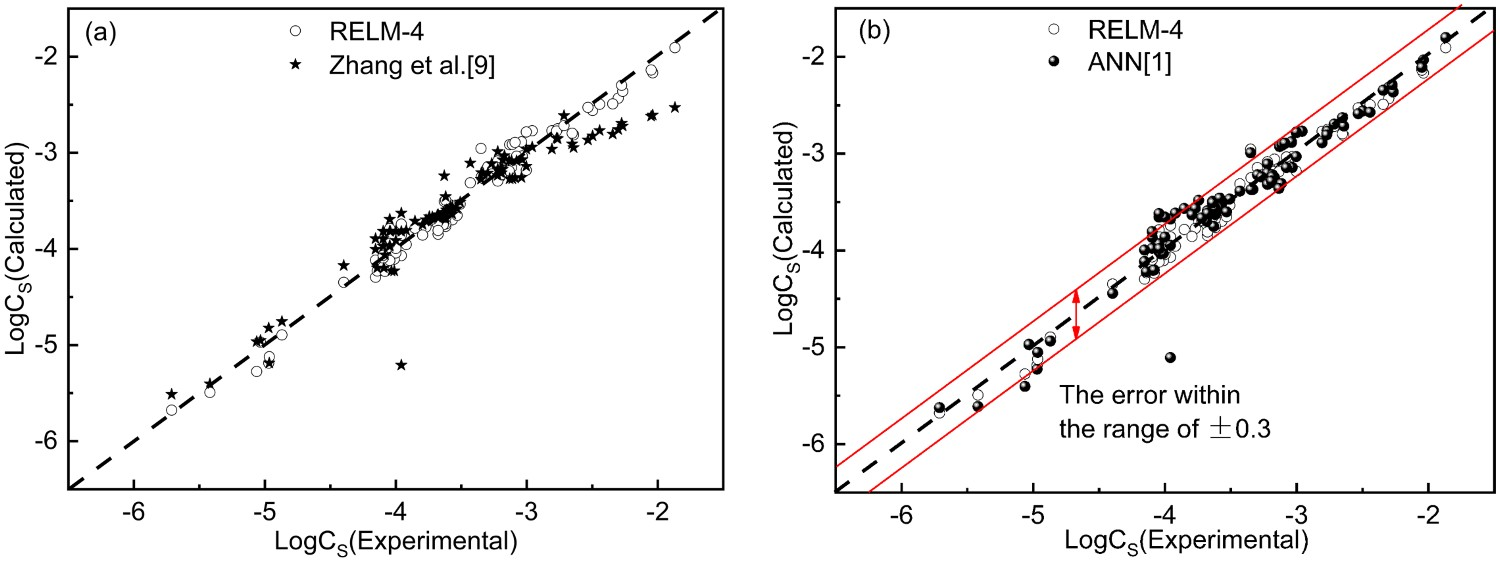

Table 5.

Comparison of the previous models.

	Sosinsky et al.’s model [7]	Young et al.’s model [8]	Zhang et al.’s model [9]	KTH model [11]	ANN model [1]	This work(RELM Model 4)
R ²	0.8969	0.8816	0.9094	0.8831	0.9378	0.9763
r	0.9470	0.9389	0.9536	0.9397	0.9684	0.9881
MSE	0.1032	0.1215	0.0374	0.0761	0.0346	0.0131
RMSE	0.3213	0.3485	0.1935	0.2758	0.1860	0.1143

The calculated values of sulphide capacity by Zhang et al.’s model and RELM- Model 4 are compared with the experimental values as shown in Figure 7(a). It is evident from this figure that the RELM Model 4 has higher prediction accuracy than the Zhang et al.’s model when the sulphide capacity is in the high range. The cause analysis is as follows: (1) In the RELM models, the number of neurons is large, and the model has a strong ability to process input variables. The RELM model can give a more accurate output when the input variables are close to the training samples. (2) The traditional regression model is difficult to be applied, when the relationship between the input variable and the output variable is not a direct linear correlation. However, RELM models have a strong nonlinear approximation ability, which can make the model prediction more accurate. (3) In the traditional linear regression model, the modelling process has been limited by the original features of the data (input variables). However, in the RELM models, instead of using the original features, the features of the hidden layer obtained by training network are used as new features, which is similar to the data pretreatment process, which thus brings about better prediction effect than the traditional linear regression model.

In Figure 7(b), the hit rate of the RELM Model 4 and the ANN model are 99% and 92%, respectively, when the error is within the range of ±0.3. The results show that the generalization ability of the RELM model outperforms the ANN model. Although RELM models have high prediction accuracy in this study, there still remains an error to improve. The contributing reasons could be as follows: (1) LF refining is a complicated physical and chemical process; there is a complex nonlinear relationship between the components, the temperature and the sulphide capacity. The complex process cannot be described accurately by using the RELM models. (2) In the process of obtaining the original experimental data, there are inevitably some errors of measurement and component analysis, which have a negative effect on the establishment of RELM model and the prediction results.

The Cs is a well-recognized index to evaluate the desulphurization ability of slag in the steelmaking process. Compared the results of different previous models with the current RELM models, the RELM models show the advantages of easy operation, fast speed of calculation and high accuracy of prediction. Thus, it can be used in predicting the Cs in real time under different composition and condition, which is of significance for quantifying the desulphurization ability of slag and optimizing the slag system. Meanwhile, intelligent iron/steel manufacturing has been drawing increasing attention in recent years. The calculation of Cs can be used to build a mathematical model for desulphurization in steelmaking practices. Specifically, when the Cs calculation model is obtained, a desulphurization model can be established by using the relationship between the Cs, the sulphur partition ratio, the mechanism of desulphurization, and the conservation of matter. The desulphurization model is able to realize the calculation and automatic charging of slagging agents (e.g. lime) in LF process. This will be detailed in our future work. In addition, the RELM model can also be applied to solve other multivariate, nonlinear and strong coupling problems in steelmaking practices, such as predicting the molten steel temperature and the quality of continuous-casting billets [16,33].

4. Conclusions

In the present study, the RELM intelligent algorithm was applied to predict the sulphide capacity in the CaO–SiO₂–MgO–Al₂O₃ slag system under various conditions and the following conclusions can be drawn.

Based on the analysis of Pearson correlation coefficient between the Cs and (wt-%MgO), the results indicated that the Cs is weakly correlated with the (wt-%MgO). Meanwhile, the computation speed and the RMSE of RELM models had little change with or without the (wt-%MgO). Thus, the (wt-%MgO) showed relatively little effect on the calculation of Cs by using RELM models.

The activation function of sinusoidal has shown better performance in the RELM models. The comparison results showed that the sulphide capacity values of RELM Model 1 and RELM Model 4 are found in good agreement with the experimental results. When the errors between the predictive value and the experimental value were within ±0.3, the hit rate of both Model 1 and Model 4 were 99%.

The RELM Model 4 tends to be more effective when the sulphide capacity is in the high range. The hit rate of the RELM Model 4 and the ANN model were 99% and 92%, when the error was within the range of ±0.3. The RELM model demonstrated better robustness and higher prediction accuracy.

The RELM model is feasible to calculate the Cs of the CaO–SiO₂–MgO–Al₂O₃ slag system with the advantage of easy operation, fast speed of calculation and high accuracy of prediction. Meanwhile, according to the calculation results of Cs based on RELM, the desulphurization ability of slag can be quantified and optimized, and thus a good foundation can be laid for the development of a mathematical desulphurization model, which is of great benefit to the intelligent control of steelmaking process.

Footnotes

Disclosure statement

No potential conflict of interest was reported by the author(s).

References

Mostaghel

Chattopadhyay

Development of an artificial neural network to predict sulphide capacities of CaO-SiO₂-Al₂O₃-MgO slag system. ISIJ Int. 2017;57(1):114–122. doi: 10.2355/isijinternational.ISIJINT-2016-368

Berger

Pezzin

Grillo

et al. Analysis of the influence of adding CaF₂ and Na₂O to steel desulfurizing mixtures using computational thermodynamics. J Mater Res Technol. 2019;8(5):4651–4658. doi: 10.1016/j.jmrt.2019.08.009

Matsubae

Kubo

Nagasaka

Recycling effects of residual slag after magnetic separation for phosphorus recovery from hot metal dephosphorization slag. ISIJ Int. 2010;50(1):65–70. doi: 10.2355/isijinternational.50.65

Duan

Shi

Wang

et al. Investigation of desulfurization of inconel 718 superalloys by ESR type slags with different TiO₂ content. J Mater Res Technol. 2019;8(3):2508–2516. doi: 10.1016/j.jmrt.2019.01.027

Fincham

Richardson

The behaviour of sulphur in silicate and aluminate melts. P Roy Soc A. 1954;223(1152):40–62.

Duffy

Ingram

Optical basicity-IV: influence of electro negativity on the Lewis basicity and solvent properties of molten oxyanion salts and glasses. J Inorg Nucl Chem. 1975;37(5):1203–1206. doi: 10.1016/0022-1902(75)80469-6

Sosinky

Sommerville

The composition and temperature dependence of the sulfide capacity of metallurgical slags. Metall Mater Trans B. 1986;17(2):331–337. doi: 10.1007/BF02655080

Young

Duffy

Hassall

et al. Use of optical basicity concept for determining phosphorus and sulphur slag-metal partition. Ironmak Steelmak. 1992;19(3):201–219.

Zhang

Chou

Pal

Estimation of sulfide capacities of multicomponent slags using optical basicity. ISIJ Int. 2013;53(5):761–767. doi: 10.2355/isijinternational.53.761

10.

Bale

Chartrand

Degterov

et al. Factsage thermo-chemical software and databases. Comput Coup Pha Diag Therm. 2002;26(2):189–228.

11.

Nzotta

Seetharaman

Sulphide capacities in some multi component slag system. ISIJ Int. 1998;38(11):1170–1179. doi: 10.2355/isijinternational.38.1170

12.

Pezzin

Berger

Grillo

et al. Analysis of the influence of the solid and liquid phases on steel desulfurization with slags from the CaO-Al₂O₃ systems using computational thermodynamics. J Mater Res Technol. 2020;9(1):838–846. doi: 10.1016/j.jmrt.2019.11.023

13.

Derin

Suzuki

Tanaka

Sulphide capacity prediction of molten slags by using a neural network approach. ISIJ Int. 2010;50(8):1059–1063. doi: 10.2355/isijinternational.50.1059

14.

Huang

Song

et al. Trends in extreme learning machines: a review. Neural Netw. 2015;61:32–48. doi: 10.1016/j.neunet.2014.10.001

15.

Huang

Zhu

Siew

Extreme learning machine: theory and applications. Neurocomputing. 2006;70:489–501. doi: 10.1016/j.neucom.2005.12.126

16.

Chen

Yang

et al. Quality prediction of the continuous casting bloom based on the extreme learning machine. Chin J Eng-en. 2018;40(7):815–821.

17.

Guan

Tang

Wang

et al. Extreme learning machine with superpixel-guided composite kernels for SAR image classification. IEICE T Inf Syst. 2018;E101-D(6):1703–1706. doi: 10.1587/transinf.2017EDL8281

18.

Zou

Zhang

Liu

et al. Prediction of central carbon segregation in continuous casting billet using a regularized extreme learning machine model. Metals. 2019;9(12):1312. doi: 10.3390/met9121312

19.

Carl

Sulfide capacity in ladle slag at steelmaking temperatures. Metall Mater Trans B. 2015;46B:2609–2615.

20.

Drakaliysky

Seetharaman

An experimental study of the sulphide capacities in the system Al₂O₃-CaO-SiO₂ . Can Metall Quart. 1997;36(2):115–120.

21.

Ohta

Kubo

Morita

Effects of CaF₂, MgO and SiO₂ addition on sulfide capacities of the CaO-Al₂O₃ slag. Tetsu-to-Hagane. 2003;89(7):742–749. doi: 10.2355/tetsutohagane1955.89.7_742

22.

Hayakawa

Hasegawa

Oh-nuki

et al. Sulphide capacities of CaO-SiO₂-Al₂O₃-MgO slags. Steel Res Int. 2006;77(1):14–20. doi: 10.1002/srin.200606124

23.

Taniguchi

Sano

Seetharaman

Sulphide capacities of CaO-Al₂O₃-SiO₂-MgO-MnO slags in the temperature range 1673–1773K. ISIJ Int. 2009;49(2):156–163. doi: 10.2355/isijinternational.49.156

24.

Hino

Kitagawa

Banya

Sulphide capacities of CaO-Al₂O₃-MgO and CaO-Al₂O₃-SiO₂ slags. ISIJ Int. 1993;33(1):36–42. doi: 10.2355/isijinternational.33.36

25.

Chen

et al. Sulphide capacity of CaO-SiO₂-Al₂O₃-MgO system relevant to low MgO blast furnace slags. ISIJ Int. 2016;56(12):2126–2131. doi: 10.2355/isijinternational.ISIJINT-2016-274

26.

Seo

Kim

The sulphide capacity of CaO-SiO₂-Al₂O₃-MgO(-FeO) smelting reduction slags. Steel Res Int. 1999;70(6):203–208. doi: 10.1002/srin.199905627

27.

Adolfo

Carl

Experimental determination of sulphide capacities of blast furnace slags with higher MgO contents. Ironmak Steelmak. 2019;46(3):207–210. doi: 10.1080/03019233.2017.1366089

28.

Adolfo

Shu

Sulfide capacities in the Al₂O₃-CaO-MgO-SiO₂ system. Steel Res Int. 2018;89:1–7.

29.

Shankar

Gornerup

Lahiri

et al. Sulfide capacity of high alumina blast furnace slags. Metall Mater Trans B. 2006;37B:941–947. doi: 10.1007/BF02735016

30.

Sheng

Xie

Pan

Probability theory and mathematical statistics. Beijing: Higher Education Press; 2008.

31.

Huang

Zhu

Siew

Extreme learning machine: a new learning scheme of feed forward neural networks. In Proceedings of the international joint conference on neural networks (IJCNN 2004); 2004 July 25–29; Budapest, Hungary. p. 985–990.

32.

Deng

Zheng

Chen

et al. Research on extreme learning of neural networks. Chin J Comput. 2010;33(2):279–287. doi: 10.3724/SP.J.1016.2010.00279

33.

Tian

Mao

Wang

Hybrid modeling of molten steel temperature prediction in LF. ISIJ Int. 2008;48(1):58–62. doi: 10.2355/isijinternational.48.58

Sulphide capacity prediction of CaO–SiO 2 –MgO–Al 2 O 3 slag system by using regularized extreme learning machine

Abstract

1. Introduction

2. Cs calculation using RELM model

2.1. Analysing of database and data

Experimental data used for the RELM prediction of Cs.

The calculation results of P-value between Log Cs and input parameters.

Definition of RELM models 1–6 according to the input variables and activation functions.

(13) (14) (15) where Np is the number of the total data set; y is the value of Cs; is the average value of the Cs; the ‘exp’ means the experimental values; the ‘cal’ means the calculated values. 3. Results and discussion

3.1. The effect of MgO and activation function on Cs

Table 4.

Results of various models.

Comparison of the previous models.

Footnotes

Disclosure statement

References

(13) (14) (15) where N_p is the number of the total data set; y is the value of Cs; is the average value of the Cs; the ‘exp’ means the experimental values; the ‘cal’ means the calculated values.
3. Results and discussion