Prediction of properties over the length of the coil during thermo-mechanical processing using DNN

Abstract

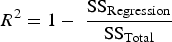
Certain mechanical properties of steel, such as elongation percentage, yield strength and ultimate tensile strength, form the basis for classification of steel coils into various categories. Methods to improve the prediction of such properties, using multiple chemical and physical process parameters, have remained an integral area of research in steel plants. In this paper, an important parameter, that is, the run-out table cooling profile of a hot strip mill coil, is considered along with the customary process parameters. This additional parameter allows a deep neural network-based model to predict the mechanical properties of steel for multiple segments along the entire length of the coil instead of the established single-segment property prediction process with very high R ² value.

Introduction

Owing to its high tensile strength, low cost and recyclable life-span, steel is one of the most important green materials consumed worldwide. Its versatility makes it a crucial material for construction and engineering purposes. According to various end product requirements, steel products can be broadly classified into bars, rods and sheets. While bars and rods are usually hot-rolled, steel sheets may either be a byproduct of the hot-rolled process or the cold-rolled process [1]. In this study, we concentrate on the hot rolled steel sheets produced by the hot strip mill. The hot strip mill produces thin sheets from slabs of steel using a process called hot rolling [2,3]. Slabs from the yard are cold and dense. Hence, they are required to be reheated (1100–1250 °C) and soaked before they can be rolled into thin sheets. Heat soaking the slabs allows the micro- alloying elements of steel [4] to homogenize and go into solutions. Once the slabs are optimally heated, they become malleable enough to break the slab cast structure and be rolled into intermediate sheets of approximately 30 mm thickness during which temperature might come down to 1030 °C via the roughing mill. Finally, sets of rollers in the finishing mill reduce the sheet thickness to the desired value (2–12 mm).

The hot strip mill (HSM) process distinctly shows that the mechanical properties of steel sheets are governed by a complex interaction of various physical and chemical process parameters. In addition to the type of alloying element, the quantity of alloying element being added to the steel is also influence the properties of the steel.

Carbon, which is usually known to aid in the strength of steel, may also have an adverse effect on its drawability [5]. Silicon, manganese and micro-alloying elements like Nb, V and Ti cause increase in strength. It is to be noted that chemical composition and processing parameters also influence the presence of harder and softer phases in steel which governs the combination of different mechanical properties. The impact of various chemical elements, process parameters and the final mechanical properties have a convoluted non-linear relationship which makes it difficult to efficiently control and predict the required mechanical properties via traditional mathematical models.

Steel property analysis also shows that the final properties of steel depend on finish rolling temperature (FRT), which influences the size of the final structure. On the other hand, the terminal sheet coiling temperature (CT) is chosen to control various phases and precipitation in the final micro-structure, which also greatly affects the final mechanical characteristics of steel. It has been observed that not only the initial FRT and final CT but the thermal history between these two points has a lot of influence on the final properties. Therefore, being the mediator between the finishing mill and the coiling section, it is discernible that the run-out table (ROT) cooling pattern becomes metallurgically critical in obtaining the desired temperature of the final product (200–650 °C) [6]. As demonstrated by Figure 1, the production grade of various categories of steel distinctly depends on the type of coil cooling pattern used at the ROT.

Figure 1.

Effect of coil cooling profile on type of steel (Lawrence et al. (1996); Mukhopadhyay and Sikdar (2005)).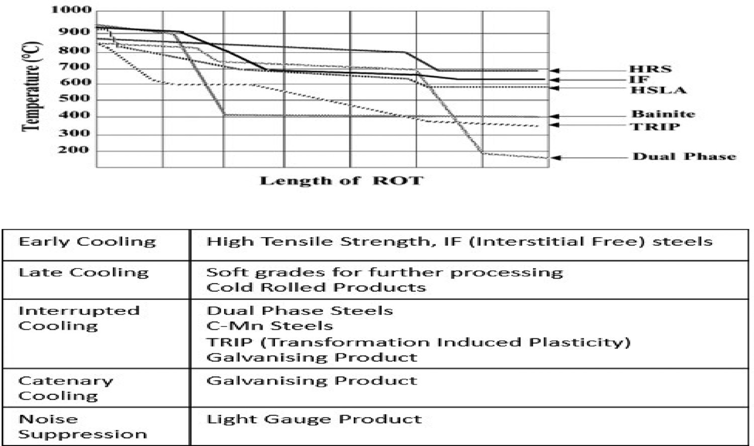

The steel industry has seen a recent rise in the usage of multiple machine learning algorithms for solving various prediction problems. Artificial Neural Networks (ANNs) [7,8] and deep learning models use distinctive training algorithms which can overcome the difficulties faced by traditional mathematical models. Thus, the usage of machine learning algorithms to improve the efficiency of the steel making process has gained utmost importance in steel industries from all over the world.

Zhen-Hua [9] mentioned that GA-ANN has been used for bending force prediction in the hot strip mill. This model can be employed for on-line controlling and rolling schedule optimization.

Mahdi et al. [10] used a neural network-based model which is suitable for automatic control as well as optimization of rolling schedule. Zhang et al. [11] presented a machine learning approach to foretell the byproduct gas holder level and to sustain the gas holder within the prescribed safety standards. Lieber et al. [12] depicted how supervised and unsupervised learning algorithms can help to identify intriguing patterns and production features within interlinked manufacturing processes of the steel rolling mill.

The FRT and CT have large impact on the microstructure which includes ferrite and pearlite percentage, ferrite grain size and pearlite spacing. All these microstructure parameters have bearings on the mechanical properties of steel which are discussed in detail in [13].

Mukhopadhyay and Iqbal [14] used ANNs to determine the mechanical properties of hot- rolled steel. In 2017, Lalam et al. [15] went ahead to further use the application of ANN by monitoring the mechanical properties in the continuous galvanizing line of cold-rolled steel coils. Development of a mill load prediction model based on neural network has been done by Yang et al. [16] while Agrawal and Choudhary [17] modelled an ensemble data mining predictor for calculating fatigue strength of steel.

Mohanty et al. [18,19] have used ANN for valuation of mechanical properties of hot rolled and cold rolled steels. It has also helped in improving the understanding about various metallurgical phenomena takes place during rolling. Mohanty and Bhattacharjee [20] explained in detail the success of ANN in steel industry in predicting and controlling processes by understanding the physics behind it. Mohanty et al. [21] has shown ANN could be used in estimating and optimizing properties of microalloyed steel,, the result has been validated by thermodynamic calculation and plant trial. It has also been used to design alloys of different types of steels. ANN has also been used in combination with GA for designing cold rolled steels taking chemical composition and process parameters as inputs [22].

In Flux-Cored Arc Welding (FCAW) process, using ANN Mazumdar et al. [23] has studies the importance of welding parameters with respect to bead geometry and Heat Affected Zone (HAZ). Using ANN, the weight of all the variables on the properties of the weld zone have been analysed and found to be in consistent with the existing knowledge. Koley et al. [24] has also used ANN for predicting electrical resistivity. He has also mentioned that among the chemical composition, carbon is the most significant element to increase resistivity accompanied by manganese and silicon. Reddy et al. [25] noted that the output properties of hot-rolled steel have a high correlation with the finish rolling temperature (FRT) and coiling temperature (CT) of that coil. However, it was also found that for a particular combination of FRT and CT, the output mechanical properties are highly influenced by the process via which the coil is cooled, i.e. the cooling profile of the coil. By controlling the cooling rate the temperature of the coil as it traverses the run-out table (ROT) is controlled and the desired mechanical properties of a coil are achieved. Multiple research has been carried out to identify model equations for optimum cooling conditions of a particular grade of steel. By developing a self-learning strategy for laminar cooling control, the difference between the calculated steel temperature and the observed one at coiler entrance can be reduced [26].

Yahiro et al. [27] presented a self-adapting model which predicted the coil temperature and iteratively approximated the amount of water flow required to achieve that temperature.

Before the down coiler in hot strip mill, the heat transfer phenomenon during laminar cooling of the run-out-table (ROT) is a key metallurgical process for maintaining the quality of the steel strip. Residual stress forms because of the large variation of the temperature along the strip and results in the strip distortion [28].

The above research areas portray the significance of the ROT cooling pattern on the final mechanical properties of steel.

For an established ROT cooling pattern of a given grade of steel, a sensor computed cooling rate (CR) is also provided. Though the CR successfully captures the coil strip temperature on the ROT to a large extent, it is noted that the measured CR value is essentially the cooling rate of the ‘tail-end’ segment of the steel coil. The base assumption for using the measured CR value for the entire length of the coil, is that the cooling profile of the coil is completely homogeneous. Practically, however, the thin sheets from the hot strip mill (HSM) spread across a few kilometres when it enters the ROT. Hence, the cooling pattern may vary along the length of the coil, i.e. from the tail-end to the head-end. In this paper, we have added the ROT cooling pattern data as a supplementary parameter along with other necessary process parameters. Via this approach, we have analysed the variation in the mechanical properties of steel — elongation percentage (EL), yield strength (YS) and ultimate tensile strength (UTS) — along the length of the steel coil. The rest of the paper is organized as follows. Section 2 discloses the proposed approach which includes process description, experimental and modelling methodology. Performance, test and validation of the model is given in Section 3 and final observations are given in Section 4.

Materials and methods

The proposed approach

In this part we briefly delineate the run-out table (ROT) cooling facility at Tata Steel, Jamshedpur, India. After presenting an overview of the coil cooling pattern data attained from the ROT, a detailed procedure for incorporating the cooling pattern as an additional parameter is discussed. On interlinking the cooling pattern with the other process parameters, the proposed approach for the deep neural network model is explained.

Run-out table (ROT)

At Tata Steel, the ROT is equipped with a laminar water-cooling facility consisting of 24 top nozzles and 24 bottom nozzles. The combination of these top and bottom nozzles influences the coil cooling profile, as a result affects the mechanical properties of the coil. To extract the cooling pattern data for various segments along the length of the steel coil, it is necessary to understand the structural design of the ROT (Figure 2).

Figure 2.

Schematic diagram of the run-out table at the Tata Steel Plant in Jamshedpur, India (Mukhopadhyay and Sikdar (2005)).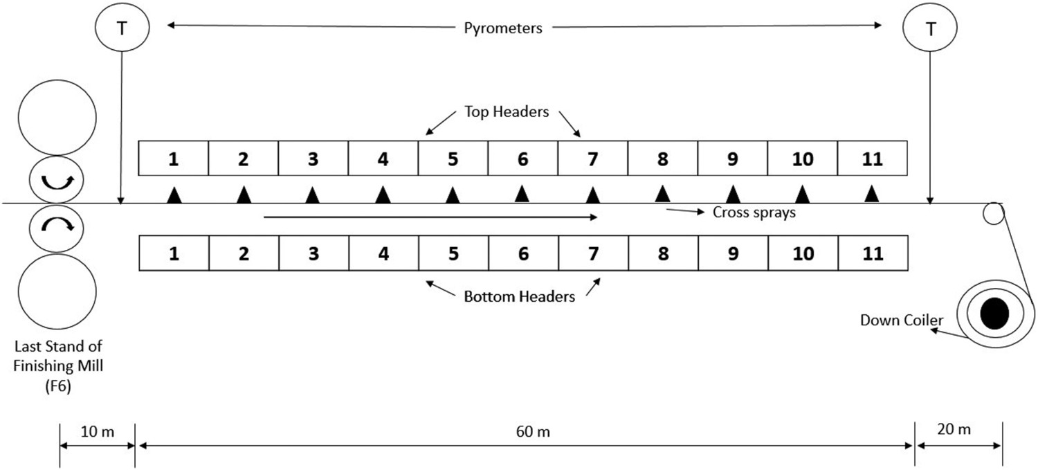

Placed on 227 rollers and spreading across approximately 60 m in length, the ROT has 24 top and bottom water cooling headers that are grouped into 11 water banks or zones – 2 headers in each of the 10 macro zones; 4 headers in the single micro zone. Each top and bottom header are controlled via a solenoid valve. The water flow rate of each header is efficiently streamlined to 3080 m³ h⁻¹ with a spray width of 1620 mm and a pressure of 0.7 bar. While the top cooling headers are spread out along the entire length of the ROT, the bottom ones are placed within the table rollers [13]. This setup guarantees consistency in water distribution on either side of the steel sheet. As a result, the cooling profile is found to be identical along the width of the coil.

The status of the top and bottom header nozzles is represented by two separate strings, each consisting of twenty-four 0 and 1 s – 0 representing a closed water valve, and 1 representing an open one. The aforementioned nozzle snapshots are captured at regular intervals of time. Therefore, the number of cooling snapshots for a particular coil is dependent on the length of the steel sheet and the speed at which it passes through the ROT.

Experimental setup and dataset pre-processing

Plant sensors provide multiple snapshots of the ROT top and bottom nozzles for a single steel coil. This makes the ROT dataset incompatible with the coil process parameters dataset. Hence, each dataset is pre-processed and cleaned separately before undergoing the deep learning modelling stage. Details of the pre-processing and cleaning approach of both the datasets are mentioned below.

Pre-processing the process parameters dataset

Tata Steel consolidated years of physical and chemical process parameters for various grades of steel coils. Consisting of two reference columns, 16 physical parameters, 15 chemical parameters and 3 tail-end output mechanical properties, the initial process parameter dataset comprised nearly 2,50,000 data samples. Upon rudimentary cleaning, certain metallurgically less important attributes were removed from the dataset. The resultant dataset was then divided into two separate groups based on the concentration of niobium (Nb), titanium (Ti) and vanadium (V) in each coil. One dataset (non-micro alloyed) consisted of coil samples where the concentration of Nb, Ti and V were all zero, while the remaining coil samples were shifted to the second (micro alloyed) dataset. Each of the final pre-processed micro alloyed and non-micro alloyed datasets comprise nearly 35,000 data samples.

Pre-processing the ROT snapshot dataset

The initial ROT snapshot dataset was sub-divided into two parts based on the coil reference numbers present in the micro alloyed and non-micro alloyed process parameter datasets. Once the necessary coils were identified and extracted, the next step comprised of generating a single cooling sequence from the series of snapshots given for each coil sample. Table 1 depicts a sample of a cooling snapshot data as a typical coil travels along the ROT. Occasionally, sensors fail to record the top and bottom cooling snapshots at an instant. This leads to huge amounts of erroneous data samples. Optimal pre-processing of the ROT data samples eradicates this initial difficulty and allows the generation of a single cooling sequence from the series of cooling snapshots of each coil.

Table 1.

Example of the first three cooling snapshots as a typical coil traverse along the run-out-table.

Coil Id	Snapshot No.	Top Nozzle Spray Data	Bottom Nozzle Spray Data
234788	1	000011100000000000000000	000000000000000110000000
234788	2	001111000011110000000000	111111111100000000000011
234788	3	111111111111110000000000	111111100000000000001111

Generation of region-specific coil cooling sequence

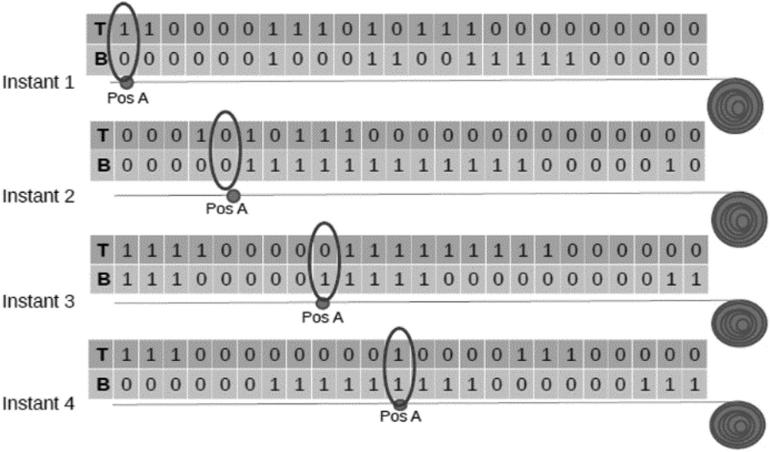
To estimate the mechanical properties of steel for multiple regions along the length of the coil, cooling sequence for each such region needs to be generated. Hence, if a coil has M top and bottom cooling snapshots and for N regions along the length of the coil the mechanical properties needs to be estimated, then N unique cooling sequences must be tracked and extracted from the M snapshots. As a prerequisite, certain information is deemed necessary: the coil length, speed of the coil as it traverses the ROT, detailed architecture of the ROT water nozzles and the ROT cooling snapshots for that region. While most of the above requirements are empirically or metallurgically available, the length of the coil, if unavailable, may be calculated based on the following equation (ρ, the density of steel, is assumed to take a constant value of (7.8 t m⁻³)): (1) For generating the cooling sequence of a region, their corresponding snapshots need to be identified. For example, the cooling snapshots for the tail-end region must appear at the end of the list of snapshots for the entire coil. However, only those extracted snapshots are deemed valid when the entire region lies on the ROT (Figure 3(a,b)). Snapshots of instances when the region is only partially on the ROT are eliminated. For a specified region length, the duration it takes to travel along the ROT is given as follows: (2)

Figure 3.

(a) Extracting valid cooling snapshots from a coil cooling profile and (b) reference for different segment of the coil.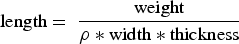

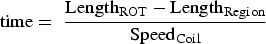
The above equation helps in identifying the time required for a region to traverse the ROT. As the snapshots are taken at regular time intervals, Equation (2) also provides information about which range of snapshots need to be extracted. For precise calculations, the region length should be limited to approximately 250 mm, assuming that the cooling profile remains homogeneous over that extent each extracted snapshot is matched with its position within the various top and bottom nozzle headers. For every such position, the corresponding top and bottom nozzle values are noted and added. Finally, all such positional values are combined to give rise to a single cooling sequence for a particular region of the coil. Figure 4 aptly summarizes how the sequence is being generated for a region, Pos A, as it moves along the ROT: 0 depicts that both the top and bottom nozzles are closed; 1 depicts that either one is open; and 2 depicts that both nozzles are open. The obtained region-specific cooling sequence captures the cooling profile for that region and aids in predicting the mechanical properties of steel at various regions along the length of the coil. However, it does not give information whether the particular region was cooled towards the beginning of the ROT or towards the end of it. To gain that data, the region-specific cooling sequence is divided into three parts of equal length – each part representing a section of the ROT. Finally, each of these three cooling sequences are encoded to make the region-specific cooling sequence data compatible with the deep neural network model structure. In this work, we have used the MD5 hash encoder [29]. The MD5 hash creates a unique 128 bit encode for a string of any length. For the same string, the MD5 has always generates the same encoded output.

Figure 4.

Schematic representation of segment tracking for region-specific cooling sequence. If ‘Pos A’ is any region along the length of the coil, then its sequence for Instant 1 is 1 + 0 = 1; for Instant 2 is 0 + 0 = 0; for Instant 3 is 0 + 1 = 1; and for Instant 4 is 1 + 1 = 2. Thus, the final cooling sequence for these four instants will become [1,0,1,2].

Deep neural network prediction model (DNN)

Two years of process data of HSM, Tata Steel was collected which consists of micro-alloyed and non-microalloyed grades of steel. Data collected from all the sections (Furnace, roughing mill, finishing mill and coiler) of HSM was synchronized over time. Matlab 2018a has been used to create the dictionaries such as rolling speed profile, coil length and ROT cooling profile using nozzle opening and closing information. These dictionaries are used to create the sequence data which is used later with other processing parameters to develop the DNN model using Python 2.7.

Upon generating the cooling profile for a region on the coil, the mechanical properties of steel for that region need to be predicted. In order to take care of the difference between the micro alloyed and non-micro alloyed process parameters, two separate deep neural network (DNN) models are created. Based on the coil reference number, the region-specific cooling sequence dataset is concatenated with either the micro alloyed or with the non-micro alloyed process parameters dataset. Since the values of the output properties present in the training dataset are explicitly for the tail-end region of the coil, both the micro and non-micro alloyed models are trained by generating the tail-end cooling sequence and dividing it into three encoded parts.

Using standard deviation normalization technique for feature scaling and adam optimization algorithm [30–33], both the micro alloyed and non-micro alloyed models use a DNN with rectified linear unit (ReLU) activation function. It is to be further noted that within each of the two dataset categories, adjustments can be made in the DNN model to increases the prediction rate for certain grades of steel.

These adjustments include changing the count of hidden layers and adjusting the learning rate of the model. Thus, in order to fully optimize the prediction rate of the mechanical output properties, four DNN models are trained for the micro alloyed and non-micro alloyed categories. The average of their predictions is taken to be the final output value. Details of the architecture of the four models are given in Figure 5.

Figure 5.

Architecture of all the four models.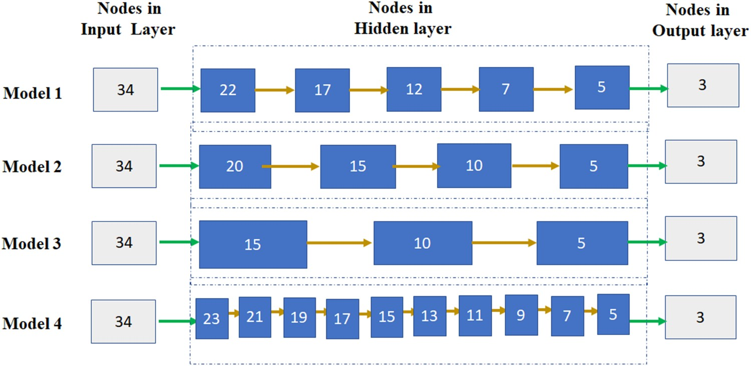

As mentioned above, four individual DNN models were developed, whose average is then taken as the predicted output. The Adam optimizer learning loss rate per iteration is shown in Figure 6. Each graph in the figure plots the learning loss of a single DNN model for both micro and non-micro alloyed coil samples. Each graph in the figure plots the training mean square error of the four DNN models for both micro and non-micro alloyed coil samples. The difference in the learning curves while keeping the same model structures shows the effectiveness of dividing the coil samples based on their micro alloying structure.

Figure 6.

Comparison of training error between the four DNN models for (a) micro alloyed and (b) non-micro alloyed steel coils.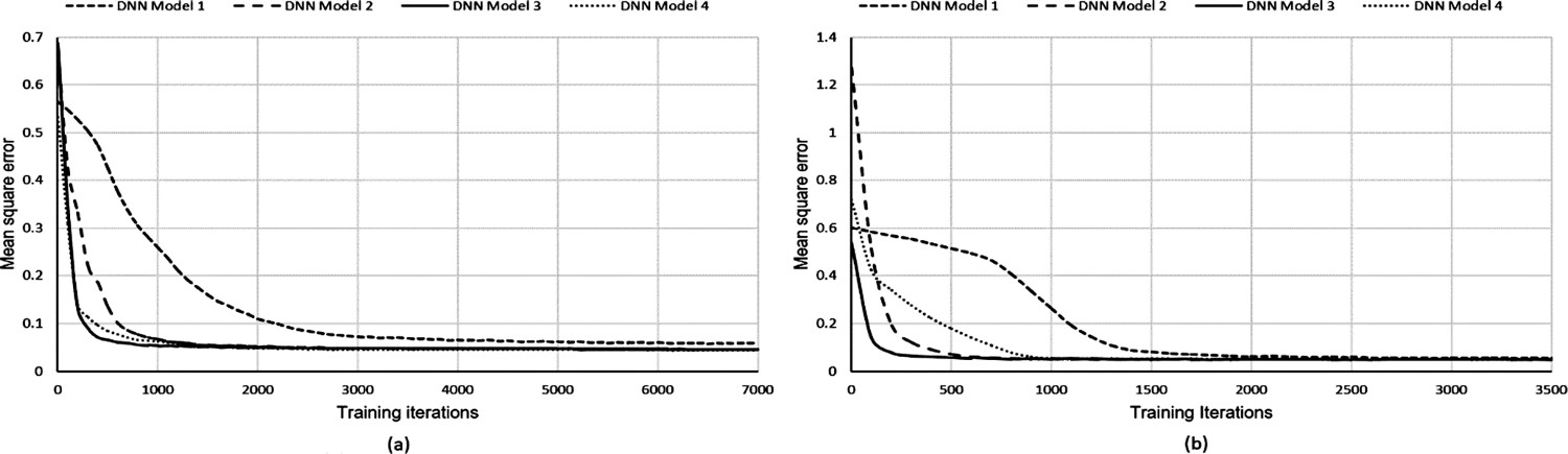

In the next section, we compare the performances of these models for the prediction tasks.

Results and discussion

Performance evaluation

Accuracy, a distinct performance criterion for classification problems, is deemed unsuitable for this regression prediction problem. In this paper, we have focused on a metric used for evaluating predictions on regression problems: the

metric [34,35]. If

is the sum squared regression error and

represents the sum squared total error, then the

error is given as: (3)

Ranging between 0 and 100%, a high

value is preferred. Tables 2 and 3 present the various

values obtained from the proposed four DNN models and other state of the art machine learning algorithms for micro alloyed and non-micro alloyed coils respectively.

Table 2.

R ² error percentage of the mechanical properties of steel for various models of micro alloyed coils.

Model name	EL (%)	YS (%)	UTS (%)
DNN Model 1 (5 hidden layers)	84.92	94.18	96.47
DNN Model 2 (4 hidden layers)	85.08	95.10	96.81
DNN Model 3 (3 hidden layers)	84.69	95.06	96.85
DNN Model 4 (9 hidden layers)	84.29	94.82	96.55
Decision Tree Model	80.72	87.32	90.07
Multilayer Perceptron Model (Tanh activation)	78.20	82.39	88.57

Table 3.

R ² error percentage of the mechanical properties of steel for various models of non-micro alloyed coils.

Model name	EL (%)	YS (%)	UTS (%)
DNN Model 1 (5 hidden layers)	85.11	92.97	97.79
DNN Model 2 (4 hidden layers)	86.64	93.43	98.11
DNN Model 3 (3 hidden layers)	85.98	93.31	98.15
DNN Model 4 (9 hidden layers)	85.05	93.14	97.94
Decision Tree	79.22	84.03	87.61
Multilayer Perceptron Model (Tanh activation)	73.18	79.34	83.94

Model consistency and performance

The objective of the training process in neural network is to have a final model that performs well both on the data that is used for training (e.g. the training dataset) and the new data set on which the model will be used to make predictions. This is done, so that the model can learn from known examples and generalize from those known examples to new examples in the future. To achieve this, methods like a train/test split or k-fold cross-validation or committee of models is used to estimate the ability of the model to generalize to new data.

The model developed here is done by using the training data and then further tested using a set of unseen data. The performance of the model during training was monitored by evaluating it on both a training dataset and validation dataset simultaneously to avoid any kind of over-fitting in the model.

The consistency and performance of the averaged DNN model was tested via K-Fold Cross Validation with 10 folds to estimate the generalization error of the chosen model configuration. In this procedure, different models are trained on k different subsets of the training data. These models are then saved and used as members of an ensemble.

Tables 4 and 5 show the consistency of the test set R ² error for the proposed machine learning models for micro and non-micro alloyed samples.

Table 4.

K-Fold cross validation model consistency via the R ² error percentage for micro alloyed steel coils.

K-Fold Number	EL	YS	UTS
Fold 1	84.11	94.10	95.93
Fold 2	86.07	94.46	96.14
Fold 3	85.15	93.81	96.10
Fold 4	85.06	95.37	97.62
Fold 5	85.68	95.04	97.07
Fold 6	84.99	94.66	96.89
Fold 7	83.49	94.42	97.66
Fold 8	85.03	95.93	95.08
Fold 9	84.21	94.57	97.03
Fold 10	84.13	95.54	97.18

Table 5.

K-Fold cross validation model consistency via the R ² error percentage for non-micro alloyed steel coils

K-Fold Number	EL	YS	UTS
Fold 1	84.73	91.86	96.32
Fold 2	84.45	93.48	98.41
Fold 3	85.91	94.18	97.30
Fold 4	86.32	93.71	98.18
Fold 5	86.25	92.46	98.69
Fold 6	85.59	94.03	97.87
Fold 7	86.34	93.40	98.92
Fold 8	86.88	93.39	97.54
Fold 9	85.62	93.74	97.83
Fold 10	84.81	91.85	98.87

Table 6 shows the

mean and standard deviation of the predicted mechanical properties for the 10-fold cross validation of the averaged micro and non-micro alloyed DNN model.

Table 6.

R ² mean and standard deviation via 10-Fold cross validation of the averaged DNN model for both micro and non-micro alloyed coils.

Micro alloyed coils
	EL	YS	UTS
Mean	84.79	94.79	96.67
Standard Deviation	0.79	0.67	0.83
Non-micro alloyed coils
	EL	YS	UTS
Mean	85.69	93.21	97.99
Standard Deviation	0.81	0.85	0.81

A successful approach in reducing the variance of neural network models is to train multiple models instead of a single model and to combine the predictions from these models. This not only reduces the variance of predictions but also results in predictions that are better than any single model. In this case a committee four different models have been developed. Each model is then used to make a prediction and the actual prediction is calculated as the average of all the four predictions.

Plant validation

The proposed approach was tested with two coil samples obtained via the daily operations of Tata Steel. The plant had deemed these two coil samples as faulty, that is, the variation in their mechanical properties along the length, exceeded the prescribed standards. Through the averaged DNN model, these two coil samples were analysed. From their process parameter and ROT datasets, the outputs were predicted for three regions along the length of the coils.

The predicted variation of the output properties via the averaged DNN model coincided with the actual plant tested output values for those three regions (Tables 7 and 8). Figure 7 depicts the variation in the predicted steel properties for twenty regions along the length for the two coil samples. The large difference in property predictions validates and boosts the importance of considering the ROT cooling profile as a salient input parameter.

Figure 7.

Variation of predicted (a) elongation length (b) yield strength and (c) ultimate tensile strength for twenty regions along the length of the two faulty steel coils provided by Tata Steel, India.

Table 7.

Averaged DNN model validation with actual plant output values for three regions along the length of the first faulty coil.

		EL (%)	YS (MPa)	UTS (MPa)
Region 1	Actual	20	407	454
Region 1	Predicted	19	400	459
Region 2	Actual	18	389	443
Region 2	Predicted	17	393	445
Region 3	Actual	17	383	458
Region 3	Predicted	16	380	462

Table 8.

Averaged DNN model validation with actual plant output values for three regions along the length of the second faulty coil.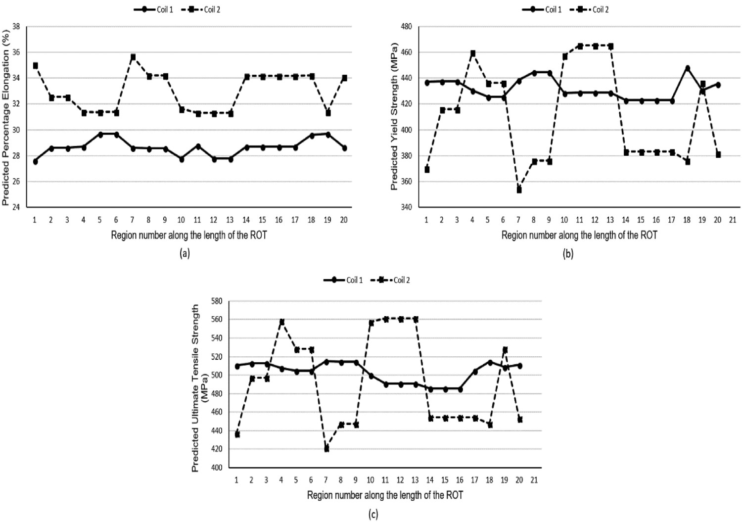

		EL (%)	YS (MPa)	UTS (MPa)
Region 1	Actual	29	378	453
Region 1	Predicted	28	381	447
Region 2	Actual	27	380	500
Region 2	Predicted	27	398	496
Region 3	Actual	28	367	472
Region 3	Predicted	28	350	485

Conclusion

The proposed deep learning model incorporates the cooling profile of a coil along with other process parameters to predict its mechanical properties, namely elongation percentage (EL), yield strength (YS) and ultimate tensile strength (UTS), along the length of the coil. Multiple region-specific cooling sequences are generated from the run-out table cooling snapshots. These sequences are then used to predict the properties for various regions along the length of the coil. Observing the difference in data distribution based on the concentrations of Nb, Ti and V, two separate neural network models are trained for micro alloyed and non-micro steel coils. Each model is then sub-divided into four DNN models and their average prediction value is considered.

Robust and consistent, the model accurately highlights the effect the run-out table cooling profile has on the properties of steel. By predicting the properties for multiple regions, the averaged DNN model also helps in identifying faulty coils which somehow failed to maintain the output specifications throughout the entire length of the coil. Having a high error of 85.221%, 94.003% and 97.334% for EL, YS and UTS respectively, the model has been approved by the technical expert and operations team of Tata Steel.

Footnotes

Acknowledgements

The authors are grateful to the management of Tata Steel for giving the approval to announce this work. The authors also acknowledge the efforts, support and involvement put by all the relevant professionals of Tata Steel to carry out this work.

Data availability

The data that endorse the discoveries of this study are accessible from the corresponding author, upon reasonable needs.

Disclosure statement

No potential conflict of interest was reported by the author(s).

References

Kawasaki

Hioki

Ohno

et al. U.S. Patent No. 4,872,245. 1989.

Ogawa

Kikuma

Higo

et al. U.S. Patent No. 5,921,127. 1999.

Bhadeshia

HKDH

Honeycombe

Steels: microstructure and properties. 4th ed. Elsevier; (2017). Thermomechanical Treatment of steels; pp. 421–455.

Karmakar

Kundu

Roy

et al. Effect of microalloying elements on austenite grain growth in Nb–Ti and Nb–V steels. Mater Manuf Processes. 2014;30(6):653–664. DOI: 10.1179/1743284713Y.0000000386.

Yunbo

Yongmei

Xianghua

et al. Modeling of microstructure evolution and mechanical properties during hot-strip rolling of Nb steels. J Univ Sci Technol Beijing Miner Metall Mater. 2008;15(4):396–401. DOI: 10.1016/S1005-8850(08)60075-4.

Hai-Jun

Li-Gang

Yong-Lin

et al. Online monitor and control of cooling temperature on run-out table of hot strip mill. Steel Res Int. 2015. DOI: 10.1002/srin.201400269.

Mitchell

TM.

Artificial neural networks. machine learning. McGraw-Hill; 1997. pp. 81–127.

Abiodun

Jantan

Omolara

et al. State-of-the-art in artificial neural network applications: A survey. Heliyon. 2018;4(11):e00938. DOI: 10.1016/j.heliyon.2018.e00938.

Wang

Gong

et al. Prediction of bending force in the hot strip rolling process using artificial neural network and genetic algorithm (ANN-GA). Int J Adv Manuf Technol. 2017;93(9–12):3325–3338. DOI: 10.1007/s00170-017-0711-5.

10.

Bagheripoor

Bisadi

Application of artificial neural networks for the prediction of roll force and roll torque in hot strip rolling process. Appl Math Model. 2013;37(7):4593–4607. DOI: 10.1016/j.apm.2012.09.070.

11.

Zhang

Zhao

Wang

et al. An optimal method for prediction and adjustment on byproduct gas holder in steel industry. Expert Syst Appl. 2011;38(4):4588–4599. DOI: 10.1016/j.eswa.2010.09.132.

12.

Lieber

Stolpe

Konrad

et al. Quality prediction in interlinked manufacturing processes based on supervised & unsupervised machine learning. Procedia CIRP. 2013;7:193–198. DOI: 10.1016/j.procir.2013.05.033.

13.

Kim

Bang

Choi

et al. Met Mater Int. 2019: 1–9. DOI: 10.1007/s12540-019-00500-2.

14.

Mukhopadhyay

Iqbal

Prediction of mechanical properties of hot rolled, low-carbon steel strips using artificial neural network. Mater Manuf Processes. 2005;20(5):793–812. DOI: 10.1081/AMP-200055140.

15.

Lalam

Tiwari

Sahoo

et al. Online prediction and monitoring of mechanical properties of industrial galvanised steel coils using neural networks. Ironmak Steelmak. 2019;46:89–96. DOI: 10.1080/03019233.2017.1342424.

16.

Yang

Linkens

Talamantes-Silva

Roll load prediction—data collection, analysis and neural network modelling. J Mater Process Technol. 2004;152(3):304–315. DOI: 10.1016/j.jmatprotec.2004.04.372.

17.

Agrawal

Choudhary

A fatigue strength predictor for steels using ensemble data mining: steel fatigue strength predictor. In Proceedings of the 25th ACM International on Conference on information and knowledge management; 2016. pp. 2497–2500. DOI: 10.1145/2983323.2983343.

18.

Mohanty

Datta

Bhattacharjee

Composition–processing–property correlation of cold rolled IF steel sheets using neural network. Mater Manuf Processes. 2008;24(1):100–105. DOI: 10.1080/10426910802543947.

19.

Mohanty

Sarkar

Jha

et al. Online mechanical property prediction system for hot rolled IF steel. Ironmaking Steelmaking. 2014;41(8):618–627. DOI: 10.1179/1743281214Y.0000000178.

20.

Mohanty

Bhattacherjee

Artificial neural network and Its application in steel industry. Hershey Pennsylvania: IGI Global; 2016. Computational approaches to materials design: theoretical and practical aspects. In: Shubhabrata

Datta

Paulo Davim

, editor. 267–300.

21.

Mohanty

Chintha

Kundu

Design optimization of microalloyed steels using thermodynamics principles and neural-network-based modeling. Metall Mater Trans A. 2018;49(6):2405–2418. DOI: 10.1007/s11661-018-4540-4.

22.

Mohanty

Bhattacharjee

Datta

Designing cold rolled IF steel sheets with optimized tensile properties using ANN and GA. Comput Mater Sci. 2011;50(8):2331–2337. DOI: 10.1016/j.commatsci.2011.03.007.

23.

Majumdar

Oraon

Laha

et al. Developing rules bases on the influence of welding parameters in FCAW process from ANN model. Int J Mech Manuf Sys. 2011;3(1):155. DOI: 10.1504/IJMMS.2010.029887.

24.

Koley

Ray

Mohanty

et al. Prediction of electrical resistivity of steel using artificial neural network. Ironmak Steelmak. 2019;46(4):383–391. DOI: 10.1080/03019233.2017.1403109.

25.

Reddy

Panigrahi

Krishnaiah

Proceedings of Seventh International Conference on Bio-inspired Computing: Theories and Applications. In Modeling mechanical properties of low carbon hot rolled steels; India: Springer; 2013. pp. 221–228. DOI: 10.1007/978-81-322-1041-2_19.

26.

Dian-yao

Jian-zhong

Liang-gui

et al. Self-learning and Its application to laminar cooling model of hot rolled strip. J Iron Steel Res Int. 2007;14(4):11–14. DOI:10.1016/S1006-706X(07)60050-8.

27.

Imanari

Fujiyama

Coiling temperature control in hot strip mill. IEEE Trans Ind Appl. 2005;125(12):1105–1112. DOI: 10.1541/ieejias.125.1105.

28.

Wang

The study of improving the strip flatness in run-out-table during laminar cooling. Int J Adv Manuf Technol. 2018;95(9-12):4419–4437. DOI: 10.1007/s00170-017-1558-5.

29.

Ross

Jackson

Miyake

et al. Stronger Password Authentication using Browser Extensions. In USENIX Security Symposium; 2005. pp. 17–32.

30.

Zhang

Improved adam optimizer for deep neural Networks. In IEEE/ACM 26th International Symposium on quality of Service (IWQoS); Banff, AB, Canada; 2018. pp. 1–2. DOI: 10.1109/IWQoS.2018.8624183.

31.

Kingma

LZ.

Adam: A Method for Stochastic optimization. In International Conference on Learning Representations (ICLR); 2015.

32.

Grus

Data Science from Scratch. Sebastopol (CA): O'Reilly; 2015. pp. 99–100. ISBN 978-1-491-90142-7.

33.

Juszczak

Tax; R DMJ Dui

PW.

Feature scaling in support vector data descriptions. In Proceedings of the 8th Annual Conference Advance School Computing and Imaging; 2002. pp. 25–30. CiteSeerX 10.1.1.100.2524.

34.

Nakagawa

Johnson

PCD

Schielzeth

The coefficient of determination R ² and intra-class correlation coefficient from generalized linear mixed-effects models revisited and expanded. J R Soc Interface. 2017;134:14. DOI: 10.1098/rsif.2017.0213.

35.

Renaud

Victoria-Feser

MP.

A robust coefficient of determination for regression. J Stat Plan Inference. 2010;140(7):1852–1862. DOI: 10.1016/j.jspi.2010.01.008.