Causality analysis and prediction of blast furnace state based on convergence cross mapping

Abstract

Blast furnace (BF) ironmaking system is a complex industrial system so this paper proposes a BF state causality analysis method based on the use of convergent cross-mapping method (CCM). This method can accurately describe the causal relationships between states at different locations in the BF system. It can also be used as a feature selection method for prediction models. After obtaining accurate causal characteristics of the BF state covariates, the BF system process theory is used for validation. The causal characteristics are used as input variables to the extreme gradient boosting model (XGboost) for predicting BF state parameters. After testing with industrial data, the model predicted an absolute error control within 2% with an accuracy of over 88%. The CCM approach mentioned in this paper is more suitable for state causal impact analysis and predictive model feature selection for BF systems.

Introduction

BF ironmaking is a complex industrial process with many physicochemical reactions, strong coupling of parameters, complex variable and nonlinearity [1–3]. There are many influencing factors in the BF smelting process, and there is a strong correlation between the influencing factors. It is necessary to make appropriate adjustments and comprehensive judgments on the production status of the BF based on the professional experience of the BF operators, but these human factors are difficult to be reflected in the BF model. The key to realizing ‘high yield, high quality, low consumption and long life’ of BF ironmaking is to timely grasp the operation state of BF, accurately analyze the reasons for the change of operation state, and stably control the appropriate operating range. The silicon content of BF molten iron is an important index to measure the quality of pig iron and the production condition of the BF [4]. At the same time, the change of silicon content directly reflects the stability of the smelting production process [5]. The BF permeability index is one of the most critical indicators to reflect the operating status of BF comprehensively [6]. Based on the permeability index, BF operators can detect and avoid BF malfunctions such as bridging or collapsing charges as soon as possible, so as to judge whether the BF is in a stable state. Gas utilization rate is an important index to measure the level of BF energy consumption [7,8]. It represents the reduction utilization rate of primary raw materials (carbon) in BF production, which directly affects the energy consumption per ton of iron. The three parameters mentioned above represent the three directions of concern for BF production: hot metal quality, running condition and utilization efficiency. Each state parameter is related to a variety of factors in the BF system. It is essential to investigate the underlying causes between the BF state variables and the other parameters to stabilize the BF smoothly. Owing to the complexity of the BF system, the interaction between parameters and the time delays, the causality of the BF condition parameters is still challenging to obtain the correct results from simple data analysis. At present, the adjustment and maintenance of BF conditions are still mainly carried out by manual experience.

Currently, there are two main directions for analyzing the relationship between BF condition and influencing parameters, which are based on data models and data-driven. Compared to data models, data-driven systems are more suitable for complex systems such as BF systems, because they do not rely on expert experience, process information, or limitations of process principles. The data-driven approach is further divided into correlation and causation. Correlation methods generally use Pearson correlation coefficients to determine the relationship between different covariates. This method applies to selecting parameters for feature engineering of traditional data prediction models. However, the correlation method has the following disadvantages compared to the causality method: 1. correlations are symmetrical, whereas causality is directional; 2. causality is time-series, whereas correlation is not necessarily. The hazards are as follows: 1. The parameters obtained by correlation analysis have poor interpretability; 2. Different methods have a significant influence on the accuracy of prediction models.

Identifying causal relationships between variables is one of the most challenging goals of scientific research. Using actual data to infer causal relationships between variables has become a valuable and economically important technique in many research areas [9–11]. Granger causality is widely used in economics, meteorological science, and neuroscience to measure the interactions between time series. Another standard method is the intercorrelation function which determines the causal relationship between variables through the similarity and temporal characteristics of two-time series [12]. However, the constraints of linear systems and parameter separability required by these methods preclude the application in BF systems. Sugihara presents the first data-driven CCM-based method that provides a new approach to reveal nonlinear causal relationships between weakly coupled variables [11]. The method exploits the characteristics of diffeomorphism between variables in nonlinear coupled systems. It transforms the original causal identification into a comparison of the mutual predictive effects of embedded manifolds. The CCM has been successfully applied in many research areas such as ecology, biology, and geosciences [13,14]. Therefore, the solution idea of the CCM applies to the BF system with a nonlinear coupling system, but there is no causal analysis for the BF status system at present.

In this paper, in order to provide a basis for the root cause tracking of BF state parameters, an modified causality method based CCM is proposed to accurately determine the causality between BF state parameters and operation parameters. At the same time, XGboost algorithm is used to verify the superiority of the causal analysis results in the parameter selection process of predicting the state parameters of BF.

The main contributions of this paper are summarized as follows: 1. for the BF system, a causal analysis method based on the CCM is used to determine the root cause of the BF state parameters and the directionality of the information flow between them; 2. the adjustment parameters (embedding dimension, lag interval) in the CCM method are judged and determined in a speciﬁc way; 3. compared with the traditional parameter selection method of prediction model, the influence of this method on the parameter selection of prediction model is verified.

The organization of the paper is as follows. Chapter 2 describes the source detection method based on the CCM, the process for selecting the optimal embedding dimension and lag interval, and the model principles of the XGboost algorithm. Chapter 3 provides an overview of the BF data states and data preparation for the three enterprises. Chapter 4 presents the embedding dimension and lag interval determination and the causal analysis of all BF states. Chapter 5 discusses the impact of the input parameters chosen by the different methods on the prediction results of the XGboost model. A summary is given in Chapter 6.

Related works

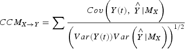
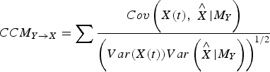
The basic idea of the CCM is that even a chaotic deterministic system is still somehow predictable in the short run. Based on the differential homeomorphism theory, this method uses the interaction characteristics of coupled variables in a nonlinear approach to provide a basis for judging the causal relationship to determine the strength and direction of the interaction between variables in a nonlinear system [15]. The CCM can be used for non-separable dynamical systems with weak to moderate coupling strength and compensates for the fact that the granger analysis method cannot be used for non-separable systems. Once proposed, the process has been widely used in ecology and neuroscience. The BF production system is a parametrically coupled, non-separable dynamic system, which fits the scope of application of the CCM method. However, the BF system is an industrial system with nonlinearity, high dimensionality, continuity, and hysteresis, which differs significantly from the traditional applicable systems.

Source model of the CCM

For deterministic systems and not completely random (e.g. BF production systems), there is a dynamics of the underlying manifold M control system (representing coherent trajectories rather than random chaotic states). For deterministic systems and not completely random (e.g. BF production systems), there is a dynamics of the underlying manifold M control system (representing coherent trajectories rather than random chaotic states). In dynamical systems theory, time series variables from the same dynamical system (e.g. BF operating covariates and state covariates) share the same attractor manifold M, so the states of each other can be estimated [16,17].

Suppose there are d-dimensional (d< = N) time-varying manifolds M in N-dimensional space. X and Y are two discrete time series with the same length L from a shared manifold M. (1) (2)

According to Takens embedding theorem, if there is a causal relationship between two variables of a dynamical system, then the shadow manifolds Mx and My of these two variables will have the property of being differentially homogeneous with the manifold M of the original system. The phase space is reconstructed using the time-delayed coordinate method. Let the dimension of the reconstructed manifold be E, and the sampling interval be τ (generally defaulted to 1). The reconstructed manifold lag time vector at time t is as follows (3) (4)

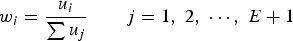
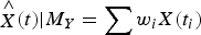
Topologically equivalent reconstructed manifolds are obtained from the above two equations. The set of X(t) is the shaded manifold M _X = {X(t)} corresponding to temporal X. The set of Y(t) is the shaded manifold M _Y = {Y(t)} corresponding to temporal Y. Based on the mutually coupled nature of the time series, M _X and M _Y exhibit a one-to-one mapping relationship in the local region. At time t, the CCM method uses the nearest point of the Y(t) mapped value in M _X as the prediction result of X(t) and measures the causality in the Y to X direction by the accuracy of X(t).

First, determine the lagging coordinate vector Y(t) on 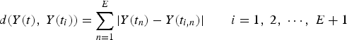M _Y at moment t, the closest moment to which is noted as t₁, and use t₁, t₂, … , t_E+1 denotes the E+1 nearest neighbour nodes of Y(t) and corresponds to the E+1 closest neighbor nodes of X(t) on M _X. The distance of each nearest neighbour node from Y(t) is solved using the Euclidean distance. (5) Next, calculate the locally weighted average weight w _i of the distance between Y(t) and i proximal points on M _Y as follows (6) (7) Finally, the formula for calculating the estimated value of X(t) obtained by M _Y is shown. (8) Similarly, a cross-mapping estimate of X to Y can be obtained by similar steps as above. Finally, the quotient of the covariance and standard deviation of the actual and estimated values is used to define a CCM correlation coefficient to measure the accuracy of the estimates. As the length of the input data sequence L increases, gradually converges to X(t), and the CCM correlation coefficient converges to a fixed value. A correlation coefficient greater than a certain threshold is considered causal for Y to X. In turn, the same analysis can be performed in the X to the Y direction. (9) (10)

Selection of the optimal embedding dimension

The choice of embedded dimension E can change the importance of attractor to characterize the original behaviour of system. An embedding dimension that is too small leads to a situation where point nearest neighbours in the state space may not represent the trustworthy nearest neighbours in the actual state space. At the same time, an embedding dimension that is too large increases the amount of unnecessary computation significantly. Professor Sugihara used the False Nearest Neighbour (FNN) to determine the optimal embedding dimension E of the manifold. Later studies and partial improvements to the FNN method made the CCM more suitable for fixed application scenarios [11]. Additional studies have used the Akaike information criterion(AIC) for the determination of the embedding dimension. Owing to the high frequency of BF production data and the considerable sample size of the data, the BIC can effectively prevent excessive model complexity caused by high model accuracy under the premise of considering the sample size. Therefore, BIC is more suitable for embedding dimension selection problem of BF data than AIC, and the BIC method is chosen in this paper to judge the embedding dimension E value.

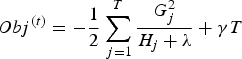
The model complexity is defined as k, the loss function B is defined, the number of samples is n, and the BIC is defined as shown in Formula (11). (11) In this paper, the X(t) autoregressive model is used to judge the best embedding dimension, and the residual sum of squares of the autoregressive model is calculated as Equation (12). (12) Let the loss function B = SSR and the model complexity k = E. When BIC(n) gets a locally smaller value, the corresponding first k value is determined as the best embedding dimension for the field.

Selection of lag time

In the BF production system, there is a specific time lag between the operation parameters and the status parameters. First, the status of the BF has a lag effect, and the current system’s status has a significant causal impact on the following status. Second, there is a time interval between the upstream variables of the BF system and the downstream variables, which is called the mechanism time lag. Finally, for the same batch of incoming raw material in the production process, there is a technical time lag due to differences in the measurement times of the different variables. For example, in the process of measuring different variables for the same batch of material, the four variables – burden structure, depth of trial rod, blast volume, and temperature of hot metal – should be measured at t₀, t₁, t₂, and t₃, respectively. The different time intervals between these four moments become the technical time lag. Time lag makes the influence of variables within a BF system vary significantly with the time interval. Time lag conditions exist for the state parameters themselves, and the operating parameters or other state parameters also have time lag conditions on the target state parameters. For the analytical perspective of the CCM dealing with a time lag, Ye proposed to add the time lag factorλbased on the CCM algorithm, and using the Y(t) at moment t can get a better prediction of X(t) at the moment t-λ [14]. During the reconstruction of manifold M, the reconstructed coordinates of the flow-form M ^λ _Y are shown in Equation (13). (13) The improved CCM algorithm is suitable for detecting causality and time lag analysis of variables in specific self-oscillating systems. However, this method is no longer applicable in BF production systems with common external disturbances. Based on the extended idea of the Cross Map Lag method mentioned above, and combined with the actual time lag of different parameters of the BF system, this paper uses the autocorrelation method and the mutual information method to analyze the time lag of the state parameters themselves and the time lag between the operating parameters and the state parameters, respectively.

The autocorrelation function (ACF) is used to measure the correlation between observations at λ unit time intervals (y_t to y_t+λ) in a time series and is given by the following Equation (14).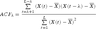 (14) where λ is the lag interval and is the mean value of the time series.

The mutual information function is a measure of the interdependence between variables [18]. The mutual information method uses the first local minimum of the mutual information function as the optimal delay time to determine the optimal time lag. Another advantage is that the mutual information method can be used independently of the embedding dimension to select the lag time. In the process of phase space reconstruction of a single variable as a time series, the strength of the lagged correlation of the variables is obtained by calculating the magnitude of the mutual information of the sampled variable series X(i) and the delayed series Y(i +λ). For the variables X(i) and Y(i+λ), the expression for the mutual information calculation is shown in expression (15).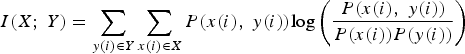 (15) where P(x(i),y(i)) is the joint probability distribution function of variables X(i) and Y(i), while P(x(i)) and P(y(i)) are the marginal probability distribution functions of variables X(i) and Y(i) respectively. For the case of time lags between the parameters of the BF system, a mutual information scheme is used to obtain the time lag values for different time lag intervals. The calculation procedure calls sklearn in python for the relevant calculations.

XGboost prediction model

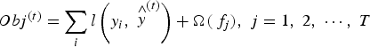
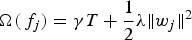
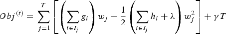
Owing to the complexity, time delay and nonlinearity of BF system, the prediction process of state parameters becomes a complex nonlinear regression problem. For such issues, XGboost, based on the improved GBDT algorithm, has good results in many engineering and process directions [19]. Therefore, the XGboost model is used in this paper to predict the BF state parameter. The principle and processes are shown below. The input parameter X and the state parameter Y of the sample set are used as the input and output values of XGBoost, respectively. An additive model consisting of M decision trees is built as follows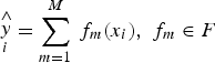 (16) where is the M^th decision tree, and all trees form the function space F. x_i is the input feature vector of the model and is the output. The objective function containing the canonical terms is defined as (17) (18) where l is the loss function, is the canonical term, T is the number of decision tree leaves, and is the penalty term for leaves and weights, and is the value of the node. Defining g_i as the first-order derivative of the squared loss function and h_i as the second-order derivative of the squared loss function, followed by a second-order Taylor expansion of the loss function l, the objective function is as follows (19) where I_j is the set of all training samples classified to the leaf node j of the tree. The final objective function is obtained by taking the partial derivative of w_j to be equal to zero as follows (20) (21) (22)

The data prediction model was calculated using the XGboost module in python, and the model evaluation was measured using a combination of accuracy, MAE, MSE, RMSE, and R2.

Data state and feature engineering for BF systems

To verify the applicability of the CCM causal analysis method in BF ironmaking production and to investigate the effect of the analysis results on the prediction model, the production data of three BFs from three different steel companies are collected for testing in this paper.

Data status

The BF ironmaking process has a long and mature history. Despite differences in the specific parameters of BFs worldwide, the basic process principles are the same. The BF data are collected from three different steel companies. The A^# BF and B^# BF are located in China, with 2500 m³ and 5500 m^3, respectively, and the A^# BF is mainly used for smelting vanadium and titanium magnetite. The C^# BF is located in Europe with a capacity of 1088 m³ and uses a bell-type distributor. Using these three BFs as examples as representatives of three different furnace capacities – large, medium, and small – all stored BF production data are collected separately. Details of the data are shown in Table 1. There are differences in the specific data and length of storage for the three BFs, as well as a slight difference in the frequency of the data. The A^# BF has the highest frequency of data, with all automated equipment data being collected at a frequency of seconds, and manual entry information being collected at tapping times and day rates. The number of fields refers to the total data collected, and the number of relevant fields refers to the number of fields retained after the manual experience has removed some of the information on auxiliary equipment that has very little relevance to BF production. Differences in the level of automation in each steel company lead to differences in the source and storage of BF production data. The results of the current data collection ensure that the majority of production data for BF ironmaking is stored.

Table 1.

Details of blast furnace production data.

BF No.	Storage time	Fields No.	Relevant Fields No.	Frequency
A^#	2018/05/01-2019/10/31	421	243	Seconds/Tapping/Days
B^#	2019/05/30-2020/08/25	156	119	Hours/Tapping/Days
C^#	2016/01/22-2020/07/5	162	104	Hours/Tapping/Days

There are differences in the production patterns of the different companies, as well as differences in the production operating conditions of the other BFs, resulting in differences in the monitoring of data on BF production, with some of the same and differential data for the three BFs listed in Table 2. The same data shows that the critical data of concern for daily BF production is recorded for each BF. Vanadium–titanium-magnetite has not been smelted in C^# BF, so [Ti] detection is not concerned in daily production. However, due to the difference in smelting raw materials, C^# BF pays great attention to the influence of [Cu] and [As] on production. The real-time class data show differences in the data recorded in the upper area of the BF due to differences in the distribution of the burden.

Table 2.

Differentiated data for the three blast furnaces.

Data type		A^#	B^#	C^#
Unique data	Real-time data	valve seat temperature	Edge temperature, Blast humidity	Distributor angle (Mckee Revolving)
Unique data	Quality inspection data	[Ti]	R3, R4, [Ti]	[Cu], [As]
Identical data	Blast temperature, Blast volume, Blast pressure, Oxygen enrichment, Burden batch, Coke rate, Coal rate, Pressure drop, CO, CO₂, [Si], [C], [Mn], [P], [S]

Feature engineering

The BF production process is complex, and there are many parameters in the BF system covering many physical and chemical reactions, so the causal analysis of the data requires the raw data to be processed first. There are various production conditions within the BF service, such as normal production, blowing out maintenance and abnormal furnace conditions, etc. Abnormal production conditions are outside the scope of this paper. This paper uses causal analysis to analyze the production status of the BF under normal production. Based on the principles of the ironmaking process, the four parameters of blast volume, blast pressure, oxygen enrichment, and coal injection are used to calibrate and reject the time interval of the abnormal production state.

In order to reduce the redundancy between the characteristic parameters, the linear correlation between the typical parameters was analyzed using Pearson correlation. The Pearson correlation coefficient(R) is in the range of [−1,1], and the higher the absolute value, the higher the correlation. Based on the purpose of reducing the redundancy of data information, the strongly correlated parameter items were selectively eliminated, and only one characteristic parameter with R greater than 0.95 was retained. The raw BF production data has various data quality issues such as outliers, missing values, and dimensional differences. The different data quality issues are dealt with separately using the Table 3 method, and the raw data are normalized. The principle of handling missing values is to use different methods to fill in the missing values when the missing amount is less than 30% and to delete them directly when the missing amount is greater than 30%. Using the box plot method, data greater than the threshold is determined as noise point. The principle of handling noise points is to replace the noise values as far as possible. The aim of standardization is to remove the influence of the dimension on the subsequent analysis. To facilitate research and comparison, the frequency of all data was standardized to 1 h.

Table 3.

Methodology for processing raw data.

Data Status	Treatment
Missing	Linear Interpolation, K-nearest neighbour classification, Proximity averaging method
Noise	Direct deletion method, Clustering algorithms
Non-standardized	Z-score standardization

Results analysis of causality

Determination of the optimal embedding dimension

For selecting embedding dimensions for the CCM method, this section uses the statsmodels library in python to calculate the embedding dimension E according to the BIC and analyses the effect of the embedding dimension on the causal results of the state parameters concerning the other parameters. The blast volume (X(i)) and gas utilization rate (Y(i)) of the B^# BF was chosen as an example for the causality analysis of the optimal embedding dimension selection. The autoregressive calculation of X(i) yields the trend graph of BIC(n), as shown in Figure 1. From Figure 1, it can be seen that as the embedding dimension increases, the BIC value shows a trend of first decreasing and then stabilizes. The first smaller value appears at k = 2, indicating that the embedding dimension equal to 2 can cover the original data information more adequately.

Figure 1.

The trend in BIC results. (Online version in colour.)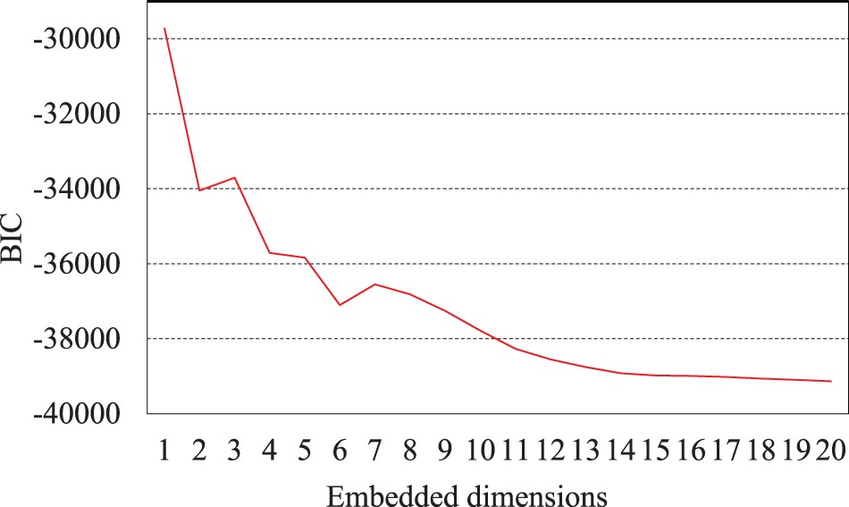

The effect of different embedding dimensions on the final causal relationship is shown in Figure 2, where the curves indicate the trend of the causal impact results (CCM values) for different directions X(i) and Y(i) with increasing data length L. (b) When the embedding dimension E is 1, the value of the CCM for causality from X(i) to Y(i) converges to 0.72 because the reconstructed manifold does not cover enough of the original information. When the embedding dimension E is 2, it can be found that the CCM value for the existence of causality from X(i) to Y(i) converges to 0.85, and the value of CCM stabilizes with the increase of length L. When the embedding dimension E is 3, the value of CCM from X(i) to Y(i) converges to 0.87, and the results are similar to those calculated with an embedding dimension E of 2. Therefore, the best embedding dimension is 2. Meanwhile, the CCM values obtained for the three embedding dimensions from Y(i) to X(i) are less than 0.2, and the causality in the direction of Y(i) to X(i) cannot be used, thus indicating that the directionality of the causality is verified. Verifying the BIC results shows that the optimal embedding dimension of the CCM method can be obtained in the BF system using the BIC method.

Figure 2.

Results of causality detection with different embedding dimensions. (Online version in colour.)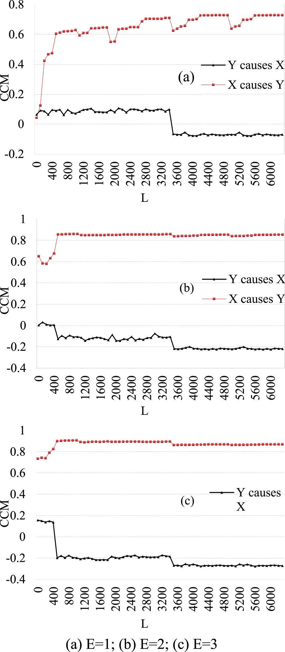

Selection of lag time

Autocorrelation analysis of state variables

The BF production status has a certain autocorrelation, where the pre-sequence time of the status variable has a significant effect on the post-sequence time. The correlation of the BF production status parameters at different time intervals is measured by the absolute value of the autocorrelation coefficient. In this paper, [Si], permeability index, and gas utilization rate of C^# BF were selected for the analysis of the autocorrelation method, and the results are shown in Figure 3. The initial value of ACF for each variable is 1. As the time interval increases, there is a significant difference in the decrease of ACF for each variable, with a threshold value of 0.7 selected and lag times of three hours, one hour, and one hour for the three parameters. Analyzing the reasons for this phenomenon, the difference in lag time between the three is due to the characteristics of BF production. In the process of BF production, the change range of permeability index and gas utilization rate is extensive, and the change frequency is high, so when the interval time is more than 2 h, the influence degree of itself will weaken rapidly. As a reflection parameter of the quality of the iron produced in the BF, [Si] itself varies more slowly than the previous two parameters, while the value of the [Si] parameter is artificially detected, resulting in a longer autocorrelation lag interval of 3 h. The results obtained using the state variable autocorrelation analysis method can be verified as correct by practical production experience.

Figure 3.

State parameter autocorrelation results. (Online version in colour.)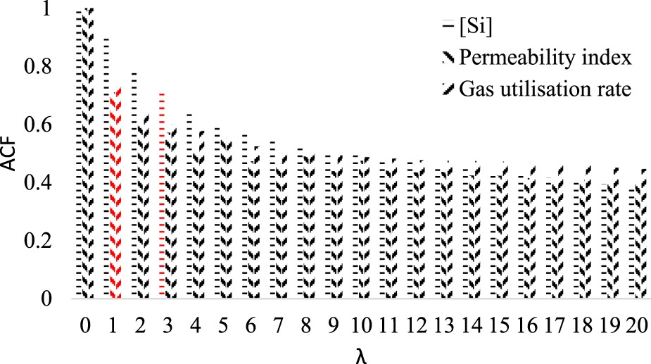

Time lag analysis of other parameters and state parameters

The time lag relationship between the other parameters and the state parameters is analyzed and the time lag interval of the CCM method is determined using the mutual information method above. The basic idea behind the choice of t_d is to make the original sample sequence and its delay sequence somewhat independent and not completely unrelated so that neighbouring data points x(i) and x(i-t_d) can be treated as independent coordinates in the phase space reconstruction. Too short t_d will result in redundant information between neighbouring components and a dramatic increase in the computational effort; too large t_d will make the neighbouring coordinates completely independent and prevent the acquisition of valid information for phase space reconstruction. In this paper, the example of the lagging interval is demonstrated using the barren gas pressure X(i) and the gas utilization rate Y(i) of the B^# BF. The mutual information of Y(t) for moment t and X(t-t_d) for moment t-t_d is shown in Figure 4. As shown in Figure 4, the first local minima of the two mutual information occur when t_d is one, and the lag period can be provisionally determined to be 1 h.

Figure 4.

Mutual information coefficients between parameters. (Online version in colour.)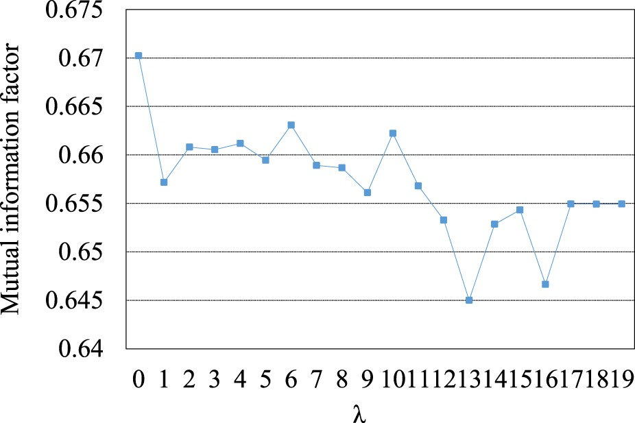

Using the above Bayesian criterion to determine that the optimal embedding dimension is 2, the causal relationship between X(i) and Y(i) was analyzed at different lag intervals t_d. The final calculation results are shown in Figure 5. As can be seen in Figure 5, the causal effect of different t_d on the causal effect of Y(i) causes X(i) is insignificant as Y(i) causes X(i) is not significant. For the causal impact of X(i) causes Y(i), when no lag time is added, the CCM value of the causal relationship between the two converges to 0.5, which is not a strong causal relationship. With the increase of the lag time TD, the CCM value increases first and then decreases. When t_d = 1, the result of the value of CCM is the largest, which is consistent with the result of mutual information. At the same time, it can be seen that the influence time of raw gas pressure on gas utilization obtained by the mutual information method conforms to the actual state of the BF system, and the excessive lag time interval weakens the degree of causal correlation.

Figure 5.

Results of causality detection with different lag intervals. (Online version in colour.)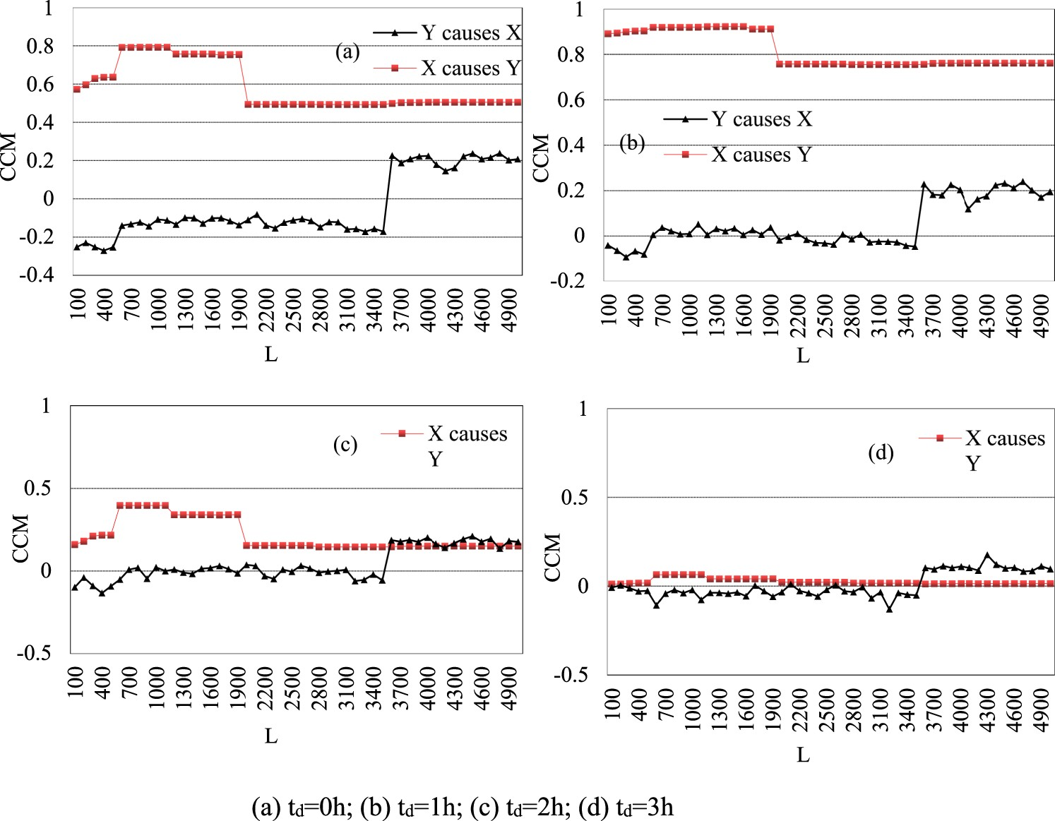

Causal analysis of state parameters

Based on the actual BF ironmaking production data collected from different steel companies, the embedding dimensions and lag times were selected in the manner described above. The causal relationships between the three state parameters of each BF and other parameters are analyzed to determine the final causality results for each state parameter.

Assuming that the time series itself has a clear unidirectional causality, with the continuous increase of the length L of the time series, the causality strength of y to x will continue to increase, and finally, converge to a stable value. The larger L indicates that the more information the time series contains, the more obvious the causality obtained by the convergent crossover method. This property is also a good indicator that the concurrent cross-mapping way can reveal the causal relationship directly. As the data length L increases, the curve of the change in the CCM values between some of the state parameters is shown in Figure 6. As can be seen from the graphs, 1. there are differences in the final test lengths due to differences in the length of data collected. 2. there is an apparent causal influence of the three state parameters and the selected parameters. The different parametric quantities during BF production all have different effects on the state parametric quantities of their respective systems, and the causal results of these three pairs of parametric amounts are in line with the actual situation of the BF system.

Figure 6.

Results of causality detection with different parameters in different companies. (Online version in colour.)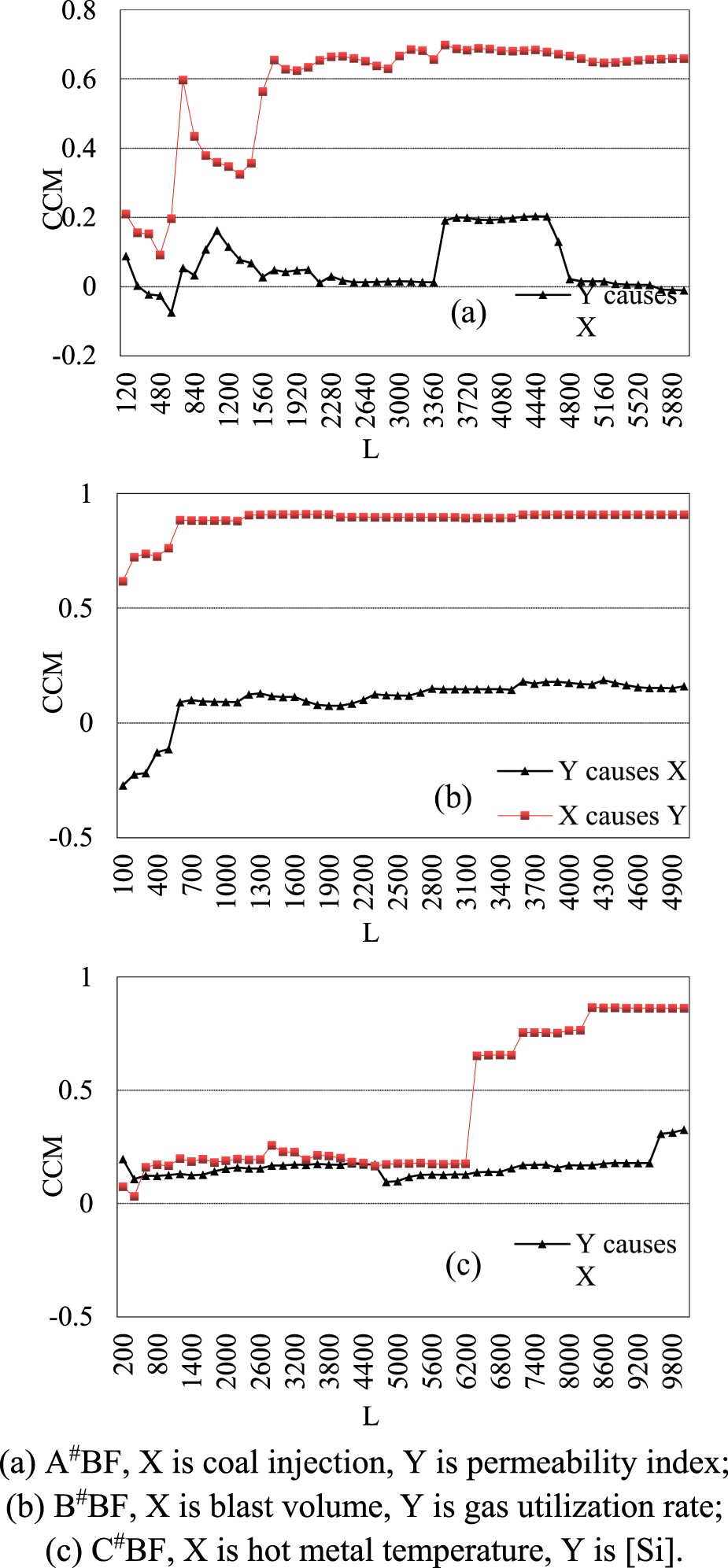

The top eighteen covariates and CCM values for each state parameter in the causal influence analysis results for the three BFs are shown in Tables 4–6. The CCM values are all stable values for the final convergence. Through the final CCM result analysis, the convergence cross-mapping method can be used to obtain the conclusion consistent with the process principle analysis.

Table 4.

Results of the causal influence of state parameters for A^#BF.

[Si]		Gas utilization rate		Permeability index
Parameter	CCM_X→Y	Parameter	CCM_X→Y	Parameter	CCM_X→Y
[Si]	0.75	Lower differential pressure	0.6	Oxygen enrichment	0.8
[Ti]	0.75	Top gas temperature	0.6	Blast volume	0.8
Coal injection	0.63	Percentage of pellet ore	0.6	Coal injection	0.8
Lower differential pressure	0.6	Central Ore Coke Ratio	0.6	Mineral consumption	0.66
Oxygen enrichment	0.6	Amount of iron	0.6	Actual blast velocity	0.8
Sealing chamber N₂	0.6	Coal injection	0.6	Amount of iron	0.8
Blast pressure	0.6	Burden batch	0.6	Top gas pressure	0.8
Burden batch	0.6	Oxygen enrichment	0.6	Hearth temperature	0.8
Total sinter	0.6	Stave cooler temperature	0.6	Stave cooler temperature	0.7
Percentage of lamp ore	0.6	Blast kinetic energy	0.55	Shaft pressure	0.7
[S]	0.6	Cooling feedwater pressure	0.5	Lower differential pressure	0.62
Top gas temperature	0.55	Standard blast velocity	0.5	Blast pressure	0.6
Pulverized coal injection	0.55	Blast volume	0.5	Oxygen post-valve pressure	0.6
Top gas pressure	0.5	pulverized coal injection	0.5	Top gas flow	0.6
Blast temperature	0.5	Mineral consumption	0.5	N₂ mains flow	0.6
Standard blast velocity	0.5	CO	0.5	Top gas temperature	0.6
Cooling return water temperature	0.45	CO₂	0.5	Coke rate	0.6
Cooling feedwater pressure	0.42	Actual blast velocity	0.5	Pulverized coal injection	0.6

Table 5.

Results of the causal influence of state parameters for B^#BF.

[Si]		Gas utilization rate		Permeability index
Parameter	CCM_X→Y	Parameter	CCM_X→Y	Parameter	CCM_X→Y
[Ti]	0.82	CO₂	0.9	Blast volume	0.8
[C]	0.75	Standard blast velocity	0.9	Blast pressure	0.8
[S]	0.6	Barren gas pressure	0.9	Top gas pressure	0.8
[Mn]	0.5	Amount of iron	0.85	Pressure drop in furnace	0.8
[P]	0.5	Top gas pressure	0.85	Standard blast velocity	0.8
Sealing chamber N₂	0.4	Blast volume	0.85	Bosh gas index	0.8
Blast pressure	0.3	Top gas flow	0.82	Top gas flow	0.8
Cooling return water Temperature	0.3	Bosh gas index	0.8	Net gas pressure	0.8
Standard blast velocity	0.25	Actual blast velocity	0.8	Blast kinetic energy	0.8
(S)	0.2	Blast pressure	0.8	H₂	0.8
(TiO₂)	0.2	Blast kinetic energy	0.78	Oxygen enrichment	0.8
Coal injection	0.2	Burden batch	0.6	Cooling return water temperature	0.65
Hearth bottom temperature difference	0.2	Blast temperature	0.6	Sealing chamber N₂	0.6
Stave cooler temperature difference	0.2	Lower differential pressure	0.6	Barren gas pressure	0.6
Burden batch	0.2	Central Ore Coke Ratio	0.6	Lower differential pressure	0.6
H₂	0.15	Thermal road	0.4	N₂	0.6
Blast temperature	0.15	Oxygen enrichment	0.4	Burden batch	0.6
(FeO)	0.15	Pressure drop in furnace	0.4	Blast temperature	0.6

Table 6.

Results of the causal influence of state parameters for C^#BF.

[Si]		Gas utilization rate		Permeability index
Parameter	CCM_X→Y	Parameter	CCM_X→Y	Parameter	CCM_X→Y
[Si]	0.95	CO₂	0.65	Top gas flow	0.75
Hot metal temperature	0.86	Humidification steam flow	0.62	Blast volume	0.7
[Fe]	0.8	[C]	0.6	N₂	0.7
[C]	0.65	Burden batch	0.6	Blast pressure	0.7
[P]	0.5	Blast volume	0.6	Bleeder valve opening	0.7
[Mn]	0.45	N₂	0.6	Oxygen enrichment	0.7
[Cu]	0.4	Blast pressure	0.6	Lower differential pressure	0.68
CO₂	0.4	Oxygen enrichment	0.6	Pressure drop in furnace	0.68
Iron flow rate	0.35	Bleeder valve opening	0.6	Burden batch	0.65
[S]	0.35	Hot metal temperature	0.6	Coke rate	0.6
(CaO)	0.3	Amount of iron	0.6	Blast temperature	0.6
(Al₂O₃)	0.3	Top gas pressure	0.6	Steam flow for bell	0.6
Burden batch	0.3	Top gas flow	0.55	Steam flow for large bell	0.6
Blast pressure	0.3	Blast temperature	0.5	Two bell top pressure	0.6
Blast temperature	0.3	Lower differential pressure	0.5	Coke moisture	0.6
Humidification steam flow	0.3	Pressure drop in furnace	0.5	Radar probe level left	0.6
Radar probe level left	0.3	Iron flow rate	0.5	H₂	0.5
Radar probe level right	0.3	Top gas calorific value	0.5	Amount of iron	0.5

Based on the process mechanism of the BF system itself, there are differences in the influence parameters obtained for different state parameters. The gas utilization rate is used as an example for the process mechanism analysis. In the operation of the BF production process, if the site operators need to adjust the gas utilization rate of the BF, they need to start from two directions: upper adjustment and lower adjustment. The upper adjustment mainly refers to the burden distribution system adjustment. Within a certain range, the hourly burden batch reflects changes in the burden distribution system, with adjustments to the batch changing the degree of focus on the edges and centre of the material surface. As the ore batch weight increases, gas utilization can be improved. By changing the proportion of furnace burden, the permeability of the upper charge of the BF can be changed and thus affect the gas utilization. The adjustment of ring pattern makes the charge distribution reasonable, which is the primary means to control the gas utilization. Owing to the complexity of the ring pattern, this paper uses the ore to coke ratio at different angles to reflect the change in the ring pattern, and it is worth noting that the C# BF uses a bell-type fabricator which does not involve the ring pattern. Changes in top gas pressure can alter the residence time of the gas in the BF and affect gas utilization. Lower adjustment includes blast velocity, blast kinetic energy, and tuyere, which affect gas utilization by changing the initial gas flow distribution. In general, the blast kinetic energy reflects the state of the central airflow and affects the gas utilization rate. The daily adjustment parameters of the BF are mainly the blast system, including blast volume, blast temperature, blast pressure, humidity, oxygen enrichment rate and coal injection. Any change in the blast system will affect the change in the tuyere and the gas utilization rate. Based on the different databases of each BF, there are differences in the influence parameters of the permeability index obtained in this paper. But by analyzing the same influence parameters of the three BFs, it is concluded that the upper conditioning means (Burden batch, Raw material ratios, ore coke ratio, top gas pressure) and the lower conditioning means (blast volume, oxygen enrichment rate, pressure difference, blast velocity, blast kinetic energy, coal injection) are all validated in the causal analysis of the gas utilization rate of each BF. This shows that the causal analysis method is suitable for the actual situation of the BF system. The influence parameters of [Si] contain incoming furnace data, operating data, outgoing iron data, BF monitoring data, and molten iron quality data. The influence parameters obtained from the permeability index are also validated by the BF operating experience.

For the single state parameters, the BFs of the three companies differed in terms of raw data collection though. However, it can be seen from the results that for the gas utilization rate, for example, 11 of the same variables appear in two or all of the BFs for the listed influencing parameters. For other parameters obtained separately, the calculation and analysis of data cannot be realized for other BF due to the data collection, but it does not mean that these parameters will not have an impact on the unrepresented BFs. For example, the coal injection rate of A^#BF and the belly gas volume index of B^#BF have a strong correlation in the production process, but the fact that the Bosh gas index data are not recorded for A^#BF does not mean that the real Bosh gas index of A^#BF does not have a strong causal relationship with the gas utilization rate.

For the three different state parameters, due to the differences in databases and production processes, it is obvious that the CCM results for [Si] are overall smaller than the other two values, indicating that the causal relationship between [Si] and these influencing factors are not very strong. By analysing the number of parameters with CCM values less than 0.5, [Si] has a high percentage of CCM results of 51.9%, while the other two parameters are 0. On the one hand, this is due to the fact that [Si] belongs to the inspection data with more human interference factors; on the other hand, the relationship between [Si] itself and other factors is relatively complex, and the value of the CCM decreases as the propagation path becomes longer.

Prediction of BF state parameters

The application of the causality analysis method in BF production not only yields relatively accurate causal influence correspondence, but also uses the lag time selection of its establishment process to determine the duration of the influence parameters on the state parameters. Using the lag time to determine the prediction duration, this paper defines a threshold value of 0.4 for the CCM, identifies the influence variables with the CCM values above 0.4 as input parameters to the XGboost prediction model, and makes predictions for each of the three state parameters.

Comparison between causal analysis and correlation analysis

To validate the performance of the CCM method for the selection of parameters for the prediction model, this paper uses the Pearson correlation method as a control group for analysis. Table 7 shows the absolute values of the partial Pearson correlation coefficients for the three parameters of the B^#BF. The following conclusions can be drawn from Table 7. (1) The selection parameters corresponding to different parameters are also different. (2) The overall Pearson correlation coefficient is small, and the permeability index is less than 0.2, which belongs to the weak correlation state. Only the three parameters [Ti], [C], and [S] in [Si] are more significant than 0.6, which belong to the strong correlation data, but most of them are less than 0.3, which means that the correlation between [Si] and other data are not very strong. The gas utilization rate is relatively high, but all of them are also less than 0.5, which belongs to the correlation status. Therefore, it can be found that for the real BF system data, the Pearson correlation analysis method cannot get strong correlation data. (3) In terms of specific data, the parameters obtained by Pearson deviated significantly from those obtained by causality analysis, with 38, 11, and 33% of the top 20 data being duplicate items, respectively. Moreover, Pearson correlation method only starts from the date of the characteristic parameters and the state parameters themselves, including many BF temperature state monitoring that cannot be effectively explained by the production process principles.

Table 7.

Results of Pearson correlation analysis of the state parameters of B^#BF.

[Si]		Gas utilization rate		Permeability index
Parameter	Pearson	Parameter	Pearson	Parameter	Pearson
[Ti]	0.89	CO₂	0.49	Blast temperature	0.13
[C]	0.64	[P]	0.42	Blast humidity	0.12
[S]	0.62	Electricity generation	0.39	Actual blast velocity	0.12
[Mn]	0.27	Net gas content	0.37	Sealing chamber N₂	0.11
(MnO)	0.26	Oxygen gun nitrogen volume	0.36	Pressure drop in furnace	0.11
Edge temperature	0.23	CO	0.34	Oxygen enrichment	0.10
Throat temperature	0.22	Sealing chamber N₂	0.34	Sealing chamber temperature	0.09
Amount of water pumped	0.22	Oxygen enrichment rate	0.30	Amount of iron	0.09
Oxygen enrichment rate	0.22	Thermal road	0.29	Sealing chamber water volume	0.09
Sealing chamber N₂	0.21	Sealing chamber water volume	0.27	N₂	0.08
Oxygen level	0.21	Return water temperature	0.23	[Mn]	0.08
Steam flow	0.20	H₂	0.23	Electricity generation	0.07
Steel brick temperature	0.18	Central differential pressure	0.22	Manifold oxygen	0.07
(S)	0.16	Throat temperature	0.21	Return water temperature	0.07
Top gas temperature	0.16	[Mn]	0.21	Hearth bottom temperature difference	0.06
H₂	0.15	Edge temperature	0.20	Oxygen gun nitrogen volume	0.06
TE34453	0.15	Cooling return water Temperature	0.18	1–6 cooling stave temperature difference	0.06
TE34467	0.14	TE34453	0.17	H₂	0.06

Prediction of state parameters

In order to verify the impact of causal analysis as a parameter selection method on the model predictions, three state covariates of the B^# BF were used as target values. The first 18 causal influence results and the first 18 Pearson correlation analysis results of each state covariate were used as input variables for the model to build a dataset for each state covariate prediction. This study was selected in July 2019 and in August 2020 to BF in the actual production data as the data set. The first 95% of the time range of data set was intercepted in a 9:1 ratio to divide the training and validation sets, and the last 5% of the data was used as the test set to validate and analyze the prediction results. Figure 7 shows the prediction results for the three-state parameters of the B^# BF. As can be seen from Figure 7, the causal analysis results have a clear advantage over the Pearson analysis method as a feature selection method for the XGboost prediction model, being able to predict the trend of each state variable accurately. Therefore, the causal analysis method is more promising as a feature selection tool while being better adapted to the actual production situation of BF production.

Figure 7

. Prediction results for different state parameters of B^# BF. (Online version in colour.)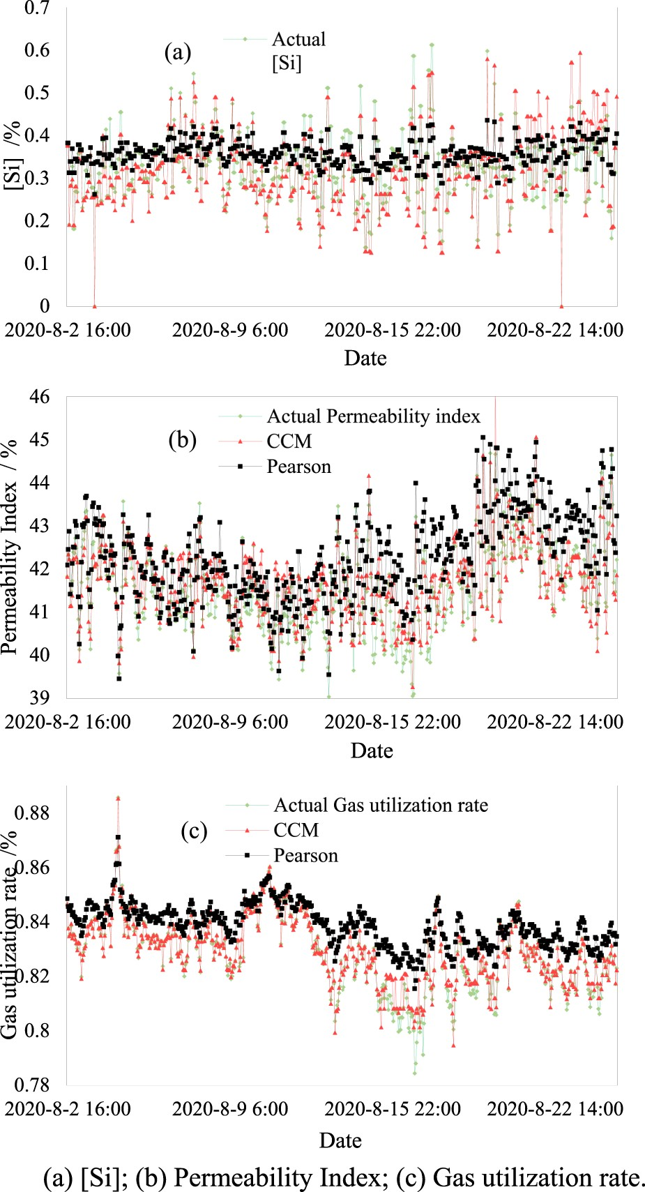

The causal influence outcome covariates of the different state covariates through the previous section were used as input parameters for each of the nine XGboost models, and the data sets were divided into training, validation, and test sets in chronological order. The prediction evaluation parameters of the model are summarized in Table 8. As shown in Table 8, for the prediction evaluation metrics of the state parameters, the input parameters determined using the causal analysis method performed well in the model predictions, with a much higher R2 and accuracy than the Pearson correlation method.

Table 8.

Evaluation of prediction results for all state parameters.

BF No.	State parameters	MAE	MSE	RMSE	R2	Accuracy
BF No.	State parameters	MAE	MSE	RMSE	R2	0.5% ([Si]5%)	1% ([Si]10%)	2% ([Si]15%)
A^# BF	[Si]	0.016	0.001	0.022	0.7	62.2	87.01	90.66
	PI	0.486	0.384	0.62	0.788	56.29	71.26	91.76
	GUR	0.396	0.571	0.755	0.842	47.50	76.11	93.71
B^# BF	[Si]	0.029	0.001	0.037	0.791	61.85	72.77	88.29
	PI	0.001	0.001	0.003	0.956	51.57	78.18	89.64
	GUR	0.217	0.129	0.378	0.874	91.68	97.04	99.63
	[Si].Pearson	0.054	0.004	0.066	0.322	41.85	52.03	58.33
	PI.Pearson	0.01	0.001	0.012	0.208	13.12	28.46	60.25
	GUR.Pearson	0.717	0.695	0.834	0.314	16.63	36.96	85.58
C^# BF	[Si]	0.052	0.006	0.074	0.874	55.91	87.79	90.06
	PI	0.275	0.934	0.791	0.892	77.5	85.12	92.05
	GUR	0.004	0.001	0.016	0.871	87.81	90.59	91.73

Note: PI = Permeability Index; GUR = Gas utilization rate.

By comparing the prediction results of state parameters of the three BFs, the XGboost model can accurately predict the changing trend of the state variables. The goodness of fit R2 is more significant than 0.7, and the MAE, MSE, and RMSE are all maintained at a high level. For the accuracy analysis of the three state covariates, the range of variation of [Si] is 5–15% due to the quality of the [Si] data itself and the large interpretation of [Si] in actual production. Ensuring that the variability of the covariates is within 2% (15% for [Si]), the accuracy of the model can all be achieved at over 85%. By using the causal analysis method to obtain the input parameters and the XGboost model, it is possible to initially predict the changing trend of the production status of different parts of the BF, which provides a basis for further research on the BF production status adjustment strategy and realizes the guidance for the operators on site.

Conclusions

In this paper, a new causal analysis model is proposed to determine the causal relationship between different production state parameters of a blast furnace. The CCM method and the XGboost model are combined to establish a causal analysis and prediction model for the BF production state. After industrial data testing, the model is able to achieve a more accurate prediction of the blast furnace production state within an absolute error range of 2%, thus enabling a preliminary prediction of the changing trend of the BF production state based on the process data.

The CCM method is used to carry out causal analysis of the three state parameters of BF production, and the causal relationship between the state parameters and the BF operating parameters is obtained. The verification of the production process experience is satisfactory. It shows that the causal analysis method applies to the data analysis of BF production states.

In the process of parameter determination for the CCM, the best embedding dimension is judged using Bayesian criteria, and the results meet the expected requirements.

In the process of judging the lags of different covariates, the autocorrelation and mutual information methods are used to analyze the correlation between the state parameters themselves and the two variables respectively, and the causal influence relationship using the lag interval is more obvious.

Based on the XGboost model, the ideal prediction results can be accurately obtained by using the causal analysis results as input parameters, and the prediction accuracy and precision are significantly improved compared to the traditional Pearson correlation coefficient selection method.

Footnotes

Acknowledgements

Thanks are given to the financial support from the Basic Research Program of the National Nature Science Foundation of China (52004096), the China NSF project (E2019209314), and Hebei Provincial Higher Education Fundamental Research Projects (JQN2020032).

Disclosure statement

No potential conflict of interest was reported by the author(s).

ORCID

Hongyang Li

Qing Lyu

References

Zhou

Guo

Wang

et al. Data-driven robust M-LS-SVR-based NARX modeling for estimation and control of molten iron quality indices in blast furnace ironmaking. IEEE T Neur Net Lear. 2017;29:4007–4021. doi:10.1109/TNNLS.2017.2749412.

Gao

Jian

Luo

SH.

Modeling of the thermal state change of blast furnace hearth with support vector machines. IEEE T Ind Electron. 2012;59:1134–1145. doi:10.1109/TIE.2011.2159693.

Kuang

Yan

et al. Numerical study of hot charge operation in ironmaking blast furnace. Miner Eng. 2014;63:45–56. doi:10.1016/j.mineng.2013.11.002.

Zhou

Zhang

et al. Autoencoder and PCA based RVFLNs modeling for multivariate molten iron quality in blast furnace ironmaking. Acta Automatica Sin. 2018;44:1799–1811.

Zhou

Robust regularized RVFLNs modeling of molten iron quality in blast furnace ironmaking. Acta Automatica Sin. 2020;46:721–733.

Yin

Zhang

Prediction model of improved multi-layer extreme learning machine for permeability index of blast furnace. Control Theory & Appl. 2016;33:1674–1684.

Zhao

et al. Gas utilization ratio prediction of blast furnace based on intelligent model. China Metall. 2021;31:93–100.

Zhang

Yin

et al. Application of the improved the ELM algorithm for prediction of blast furnace gas utilization rate. IFAC Papers OnLine. 2018;51:59–64. doi:10.1016/j.ifacol.2018.09.393.

Granger

CWJ.

Investigating causal relations by econometric models and cross-spectral methods. Econometrica. 1969;37(1969):424–438. doi:10.2307/1912791.

10.

Hiemstra

Jones

JD.

Testing for linear and nonlinear Granger causality in the stock price-volume relation. J Finance. 1994;45:1639–1664. doi:10.2307/2329266.

11.

Sugihara

May

et al. Detecting causality in complex ecosystems. Science. 2012;338:496–500. doi:10.1126/science.1227079.

12.

Bauer

Thornhill

NF.

A practical method for identifying the propagation path of plant-wide disturbances. J Process Contr. 2008;18:707–719. doi:10.1016/j.jprocont.2007.11.007.

13.

Clark

Isbell

et al. Spatial ‘convergent cross mapping’ to detect causal relationships from short time-series. Ecology. 2015;96:1174–1195. doi:10.1890/14-1479.1.

14.

Deyle

Gilarranz

et al. Distinguishing time-delayed causal interactions using convergent cross mapping. Sci Rep-UK. 2015;5(2015):1–9. doi:10.1038/srep14750.

15.

Luo

Cheng

Qiu

et al. Refifined convergent cross-mapping for disturbance propagation analysis of chemical processes. Comput Chem Eng. 2017;106:1–35. doi:10.1016/j.compchemeng.2017.03.026.

16.

Deyle

Sugihara

Generalized theorems for nonlinear state space reconstruction. PLoS One. 2011;6:1–8. doi:10.1371/journal.pone.0018295.

17.

Luo

Cheng

Qiu

et al. An improved convergent cross mapping algorithm for causality identification and time delay analysis between systemic variables under external disturbance. CIESC J. 2016;67:5122–5130. doi:10.11949/j.issn.0438-1157.20161300.

18.

Zhou

Huang

JC.

New algorithm for determining delay time by mutual information. Comput Eng Appl. 2013;49:8–10.

19.

Gong

et al. Ensemble learning based methods for crown prediction of hot-rolled strip. ISIJ Int. 2021;61:1603–1613. doi:10.2355/isijinternational.ISIJINT-2020-639.