A hybrid approach using multiple linear regression and random forest regression to predict molten steel temperature in a continuous casting tundish

Introduction

Before the 1960s, the exclusive technique for casting liquid steel into a solid shape was batch casting, which involved pouring the liquid steel into ingots later shaped by stepwise rolling or forging. After the development of continuous casting techniques, it has emerged as the primary method for steel production. According to the World Steel Association, approximately 96% of the total global crude steel production in 2021 was produced through continuous casting [1]. Continuous casting offers several advantages, including enhanced productivity and metal yield, better surface and internal steel quality, reduced energy consumption, and the product being ready for direct rolling.

The basic equipment setup for the continuous casting is illustrated in Figure 1. After secondary treatment, the liquid steel, which has chemical and thermal homogeneity, is transferred to the continuous casting machine through a ladle. The liquid metal is then transferred to the tundish, which distributes the metal into the continuous casting water-cooled moulds, where metal solidification begins. Tundish is the last metallurgical vessel through which molten metal flows before solidifying, and one of the critical process parameters determining the quality of the final steel product is the degree of superheat of the melt in the tundish and in the mould.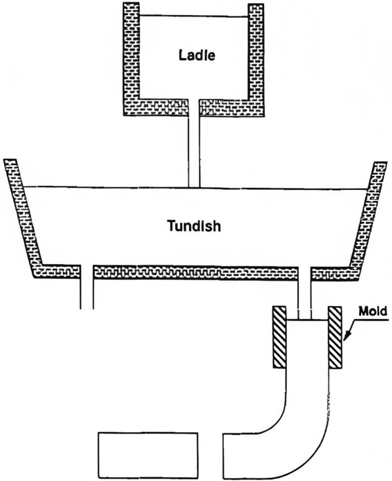OPEN IN VIEWER

Controlling the temperature of molten steel in a steelmaking plant is essential for obtaining products that meet market specifications. There is a specified suitable temperature range for each step of steelmaking, and deviations from these ranges are associated with failures that affect the product's quality and the plant's productivity.

Low steel temperatures can result in nozzle blockages due to early solidification in the tundish and consequent production interruption. Likewise, low superheat values are associated with a lower inclusion flotation efficiency.

On the other hand, temperatures above specification can result in breakouts in continuous casting and affect the structure formed during solidification. Elevated superheat of the melt results in an increase in the proportion of the columnar grain region in the solidified product [3]. The columnar zone is associated with increased segregation, which is the variation in chemical composition, according to position, of various elements dissolved in steel, such as carbon, phosphorus, and sulphur [2]. The columnar zone also correlates to a more extensive formation of midway, centreline, diagonal and longitudinal cracks in the steel product [4]. During the casting, if too much superheat is delivered to the narrow faces, then shell growth may slow down or even reverse locally, likely increasing the incidence of breakouts near the narrow faces [5].

Two predominant approaches are used for building steel temperature prediction models: physical and statistical. The former is based on thermodynamics and energy conservation, and the latter is based on regression models. The quantification of thermal losses through the physical approach involves solving energy balance equations, which require using boundary conditions and properties of complex materials. These equations can rarely be solved analytically. Gupta and Chandra [6] point out that because of the high complexity of steel cooling phenomena, the statistical approach usually achieves better results than the physical one. In addition, Sonoda et al. [7] note that the statistical approach is usually faster and less computationally demanding.

Several studies reporting the prediction of molten steel temperature can be found in the literature. Jormalainen et al. [8] used a physical model to predict the melt temperatures in the ladle and the tundish during continuous casting. Their results reached 95% accuracy within a ±7°C range for steel temperature in the tundish. Tian et al. [9] proposed an incremental learning modelling and updating method to predict molten steel temperature in a 300 tons ladle furnace using an extreme learning machine algorithm. Their results were satisfactory for production, reaching 94% accuracy within a ±5°C range. Wang et al. [10] proposed a prediction model for the final temperature of molten steel in an Ruhrstahl Heraeus vacuum degasser (RH-TOP) refining process for interstitial-free steel production. They used multiple regression models and reported a hitting probability of prediction with a deviation of ±10°C above 95%. He et al. [11] proposed a hybrid physical and statistical model based on the ladle heat status and artificial neural networks for predicting the molten steel temperature target in the ladle furnace to obtain the aimed tundish temperature. They reported an accuracy of 75.38% within a ±5°C range and 88.34% within a ±7°C range for the end ladle furnace temperature in sequence castings.

Many hybrid regression modeling strategies that combine nonparametric and parametric methods have been proposed to derive useful information from complex data. Sousa et al. [12] used a hybrid method to predict ozone concentrations and proposed a methodology based on feedforward artificial neural networks (ANN) using principal components regression (PCR) results as inputs. They reported that the feedforward ANN led to more accurate results than linear models due to the account of non-linearities. AL-Alawi et al. [13] also used a combined PCR and ANN model to predict ozone concentration levels. PCR was used to identify the most appropriate explanatory variables for the regression models, and then ANN was applied to the resulting residuals. They reported a substantial reduction in the measured root mean squared error (RMSE) and mean absolute percentage error (MAPE) in the combined forecast compared to either PCR or ANN forecasts. Adusumilli et al. [14] proposed a hybrid regression model using PCR and random forest regression (RF) for integrating Global Positioning System (GPS) and Inertial Navigation System (INS) data to bridge the GPS signal outages. Their proposed model achieved a 14%–45% improvement in prediction accuracy compared to the RF model alone.

In this work, a hybrid approach that combines multiple linear and random forest regression to predict molten steel temperature has been proposed and evaluated. The developed models predict the end temperature in the secondary refining that is expected to result in a target tundish temperature. The linear regression method models linear relations in the data, while the random forest method models non-linear relations. The models are combined using the boosting method, an ensemble technique where the models are trained sequentially using the residuals of the previous model’s results. This hybrid strategy increases the accuracy of the molten steel temperature prediction.

Methodology

The methodology employed in this work consists in multiple stages that were carried out iteratively, that is, the results attained in a stage could result in new iterations of previous stages. This methodology is based on the Cross Industry Standard Process for Data Mining (CRISP-DM) [15] and is illustrated in Figure 2.OPEN IN VIEWER

In the data collection stage, data from 2500 continuous casting heats were collected from a big steelmaking plant. Automatic online tracking systems generate the production data from each casting heat. Each record contains relevant information about the heat, such as the heat number, casting superheat at five minutes intervals, tundish and ladle’s thermal condition, and the temperatures measured at each stage of steel production.

The data preparation stage consisted of multiple feature engineering and data cleaning techniques, such as removing duplicate, empty, and incorrect data. A data balancing analysis was also performed for all categorical variables, and groups that did not have a representative amount of data compared to the other groups were removed from the data set. The choice of the variables used to fit the models was initially based on the literature and correlation analysis.

After the first model's iterations, these variables were validated with their p-value in the linear regression and the variable’s permutation importance analysis from the random forest model and the proposed model. The p-value for each variable tests the null hypothesis that its coefficient equals zero, which means that the variable does not affect the regression performance. A low p-value, usually less than 0.05, indicates that the null hypothesis can be rejected and that the predictor is likely significant to the model. The permutation feature importance is defined as the decrease in a model score when a single feature value is randomly shuffled [16]. If permuting the values causes a considerable change in the model’s accuracy, the feature is significant for the model.

Most machine learning algorithms can only handle numerical variables, so the data preparation stage also included a categorical variable transformation. The one-hot-encoding transformation was applied for the linear regression model, and the label encoding transformation was used for the random forest regression. Label encoding assigns a unique integer value to every possible value of a categorical variable [17]. On the other hand, one-hot encoding transforms an n-category nominal feature by creating binary indicator variables for the (n−1) feature levels [18]. Each observation indicates the presence (1) or absence (0) of the dichotomous binary variable [19].

Modeling

In the modeling stage, linear and random forest regression algorithms from the Scikit-learn library were initially used. Scikit-learn [20] is a general-purpose machine learning library written in Python. It provides efficient implementations of state-of-the-art algorithms, accessible to non-machine learning experts, and reusable across scientific disciplines and application fields [21].

The model aims to define the secondary refining target end temperature to meet the desired casting superheat. To simplify the use of the model in the industry, the proposed model is backward, which means that the secondary refining end temperature is the dependent variable. Since the steelmaking facility produces different steel classes, the secondary refining end temperature was transformed to secondary refining superheat, and the steel liquidus temperature was subtracted from the secondary refining end temperature before fitting the model.

A hybrid approach was proposed using a linear and random forest regression ensemble to improve the model's performance. A brief explanation of the regression models and the proposed hybrid model methodology is shown in the following paragraphs.

Multiple linear regression (MLR)

The relationship between a dependent variable

$y$ y

with

$n$ n

independent variables is named a regression model. When a regression model is a linear function of more than one independent variable, it is called a multivariate linear regression.

In general, multiple linear regression with n regressor variables is formulated as in (Eq. 1). Where

$y$ y

is the dependent variable,

$x_1\comma \; \; x_2\comma \; \ldots \comma \; x_n$ x 1 , x 2 , … , x n

are the independent variables,

$\beta _j$ β j

, j = 0, 1, … , n, are called the regression coefficients, and

$\varepsilon$ ε

is the model’s error. The model describes a hyperplane in the n-dimensional space of the regressor variables

$\lcub x_j\rcub$ { x j }

. The parameter

$\beta _j\;$ β j

represents the expected change in response y per unit change in

$x_j\;$ x j

when all the remaining independent variables

$x_j\; \lpar {i\ne j} \rpar$ x j ( i ≠ j )

are held constant [22].

$$y = \; \beta _0 + \; \beta _1x_1 + \ldots + \beta _kx_n + \varepsilon $$ y = β 0 + β 1 x 1 + … + β k x n + ε

(1)

The model error is assumed to be independent of

$x$ x

and follows a normal distribution with a mean equal to zero and constant variance.

Random forest regression (RF)

The decision tree (DT) is a predictive method in which the predictor space is divided into a set of rectangles, and then a simple model is fitted in each one. A decision tree uses a tree structure to represent several possible paths and an outcome for each path. The process of building a tree is described below [23]:

Divide the predictor space into J distinct and non-overlapping regions

$\; R_1\comma \; R_2\comma \; \ldots \comma \; R_J$ R 1 , R 2 , … , R J

.

For every observation that falls into the region

$R_J$ R J

, a prediction is made, which is the mean of the response values for the training observations on region

$R_J$ R J

.

DT can be applied to both regression and classification problems, it is often more interpretable than other models such as neural networks and are flexible enough to handle items with a mixture of real-valued and categorical features [24]. On the other hand, DT suffers from high variance, if the training data is split into two parts at random, and a DT is fitted at both halves, the models result can be very different [23].

Ensemble learning is a combination of simpler base models to build a more robust prediction model, and one technique for reducing the variance of an estimated prediction is bagging, for regression that means fitting the same regression tree many times and then averaging the results [25]. Breiman [16] introduced random forests (RF), combining several randomised decision trees and aggregating their predictions by averaging.

RF is often a collection of hundreds to thousands of trees, where each tree is grown using a bootstrap sample of the original data. Furthermore, at each node of the tree, a random subset of variables is selected to be candidates to find the best split for the node, which gives the model a second layer of randomisation and allows RF to decorrelate the trees and have low variance [26]. The RF process is described below:

Divide the original data in ntree bootstrap subsets.

Fit a tree for each bootstrap data set.

Aggregate information from the ntree for the new data prediction.

Compute an out-of-bag (OOB) error rate, which is calculated using data that is not in the bootstrap node.

Boosting hybrid approach using linear and random forest regression (LRF)

Linear regressions can only handle linear correlations between the variables, and the random forest can handle non-linear relations. The proposed hybrid regression model combines a linear model with a series of random forest models to improve the molten steel prediction accuracy.

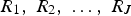
The process of training subsequent models using a previous model’s results is called boosting, another ensemble technique. The boosting technique has a slow learning approach, it does not fit a single large random forest to the data, which can lead to overfitting. Instead, it fits small trees to the residuals from the model, and the model is slowly improved in areas where it does not perform well [23].

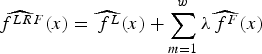
On the LRF, the linear model,

$\widehat{{\,f^L}}\lpar x \rpar$ f L ^ ( x )

, is fitted to the input data (Eq. 2), and the resulting model is used to predict the dependent variable for each instance of the same input data. The linear model's residual,

$r_i$ r i

, which contains the non-linear part of the data, is then calculated by subtracting the predicted value from the actual dependent variable value (Eq. 3).

$$\widehat{{\,f^{LRF}}}\lpar x \rpar = \; \widehat{{\,f^L}}\lpar x \rpar \; $$ f LRF ^ ( x ) = f L ^ ( x )

(2)

$$r_i = y_i-\hat{y}_i\; \; \; \; for\; all\; i\; in\; training\; set$$ r i = y i − y ^ i for all i in training set

(3)

A random forest model is then fitted to the input data, using the linear model's residuals as the training value for the dependent variable. Next, the process is repeated a predefined number of times using random forest models that are fitted using the previous model's residuals. The process is illustrated in Figure 3.OPEN IN VIEWER

Figure 3.

Hybrid approach based on boosting ensemble.

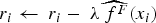
On each iteration, the LRF model is updated with the new random forest regression, Eq. 4. The model’s residual is updated as well, Eq. 5, so the next random forest is fitted on the new training data (X, r). The results of the random forests models are multiplied by a shrinkage parameter

$\lambda$ λ

, which is a positive number that controls the rate at which boosting learns. The shrinkage parameter slows the process even further, allowing a more significant number of trees to fit the residuals [23].

$$\widehat{{\,f^{LRF}}}\lpar x \rpar \leftarrow \; \widehat{{\,f^L}}\lpar x \rpar + \; \lambda \widehat{{\,f^F}}\lpar x \rpar $$ f LRF ^ ( x ) ← f L ^ ( x ) + λ f F ^ ( x )

(4)

$$r_i\leftarrow \; r_i-\; \lambda \widehat{{\,f^F}}\lpar {x_i} \rpar $$ r i ← r i − λ f F ^ ( x i )

(5)

The final model is the sum of the linear regression and all the random forest regressions multiplied by the shrinkage parameter

$\lambda$ λ

, as in Eq. 6.

$$\widehat{{\,f^{LRF}}}\lpar x \rpar = \widehat{{\,f^L}}\lpar x \rpar + \mathop \sum \limits_{m = 1}^w \lambda \widehat{{\,f^F}}\lpar x \rpar $$ f LRF ^ ( x ) = f L ^ ( x ) + ∑ m = 1 w ⁡ λ f F ^ ( x )

(6)

Model performance evaluation

The model was evaluated calculating the root mean squared error (RMSE), given by Eq. 7: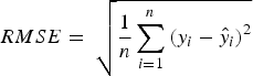

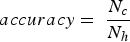
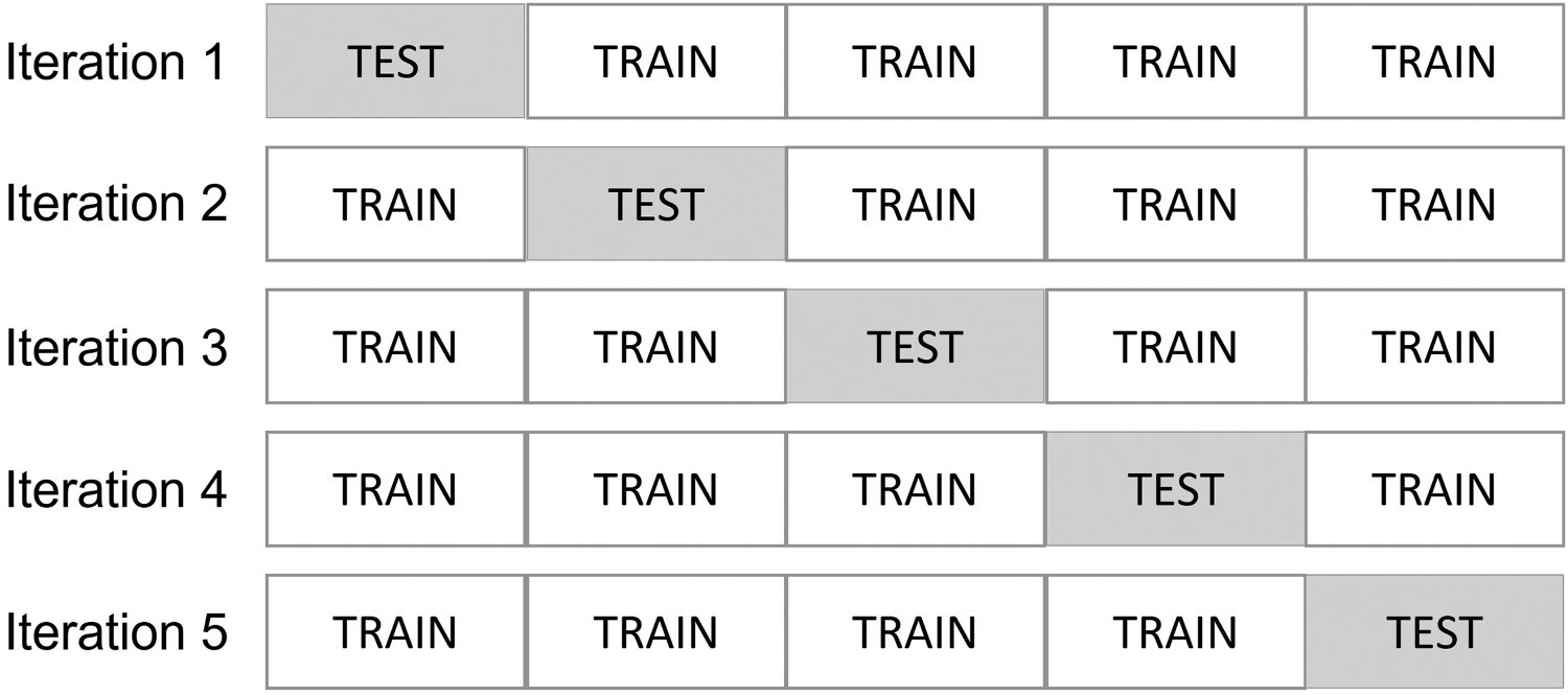
$$RMSE = \; \sqrt {\displaystyle{1 \over n}\mathop \sum \limits_{i = 1}^n {\lpar {y_i-{\hat{y}}_i} \rpar }^2} $$ RMSE = 1 n ∑ i = 1 n ⁡ ( y i − y ^ i ) 2

(7)

Where:

$n$ n

is the number of samples, the index

$i$ i

denotes the i-th sample,

$y_i$ y i

is the actual value, and

$\hat{y}_i$ y ^ i

is the predicted value.

The model was also evaluated using a custom accuracy metric that considers that a prediction is correct if its residual is less than or equal to a fixed threshold. Eq. 8 shows how the accuracy was calculated, where

$N_c\;$ N c

is the number of heats where the residuals are less than a fixed threshold, ±5 or 7°C in this work, and

$N_h\;$ N h

is the total number of heats in the data set.

$$accuracy = \; \displaystyle{{N_c} \over {N_h}}$$ accuracy = N c N h

(8)

K-fold cross-validation was used to validate if the model can generalise its prediction to an independent data set, that is, to guarantee the model is not overfitted to the training data. In this method, the data is partitioned into K roughly equally sized parts, then K – 1 of the groups are used to train the model, which is evaluated on the remaining group, see Figure 4. This procedure is repeated for all K possible choices for the held-out group, and the performance from the K runs is then averaged [27].OPEN IN VIEWER

Figure 4.

The K-fold cross-validation technique where K = 5.

Parameter tuning

The hyperparameter selection significantly impacts the model’s accuracy. Random search and grid search are methods to optimise a model’s parameters. The grid search does a complete search over a given subset of the hyperparameters space of the training algorithm and optimises the model’s parameters using a performance metric. Because the model’s parameter space may include spaces with real or unlimited values for some parameters, it is often necessary to specify a boundary to apply a grid search [28]. Grid search often suffers from high dimensional spaces. In these cases, the random search can be applied, which replaces the complete selection of all combinations by their random selection. A grid with a selection of the possible values ⁣⁣for the model parameters was made (Table 2).

OPEN IN VIEWER

Table 2.

Parameter’s description and values used to tune the LRF model.

Parameter	Parameter’s description	Tested values on parameter tuning
RF number of estimators	The number of trees in the forest	[25, 50, 150, 200, 300]
RF minimum sample split	The minimum number of samples required to split an internal node	[2, 4,10,50,100]
RF maximum leaf nodes	The maximum number of terminal nodes of the tree. If ‘None’ then unlimited number of leaf nodes [20]	[‘None’, 5,10,30,50]
RF minimum sample leaf	The minimum number of samples required to be at a leaf node	[1, 4, 10, 50,100]
RF maximum features	The number of features to consider when looking for the best split [20]	[number of features, $\sqrt {number\; of\; features}$ number of features , $\log _2number\; of\; features$ log 2 ⁡ number of features ]
RF maximum depth	The maximum depth of the tree. If ‘None’, then nodes are expanded until all leaves are pure or until all leaves contain less than the RF minimum sample split [20]	[‘None’, 10, 50, 100, 200]
LRF boosting estimators	The number of RF models fitted in LRF	[10, 25, 50, 100]
LRF learning rate	The LRF shrinkage parameter $\lpar \lambda \rpar$ ( λ )	[0.05, 0.1, 0.2, 0.3]

Since the model has many variables, the number of all the possible parameter combinations is 150.000. Considering a 5-fold cross-validation, the model would be fitted 750.000 times, generating high computational demand. Randomised parameter optimisation was performed to reduce the number of iterations, in which 1.500 random combinations of parameters were generated, and the model was fitted with each of these combinations. The number of parameter values to be tested was reduced based on the best parameters obtained from the randomised parameter optimisation. Subsequently, the complete grid search was performed, and the optimised parameter’s value was selected.

Results and discussion

The results of the evaluations carried out in this work revealed that the proposed LRF model achieves superior performance for the studied dataset compared to multiple linear or random forest regression individually. Table 3 shows the RMSE and accuracy metrics results for the three regression models. The multiple linear model consistently achieved better results compared to the random forest model for all metrics, indicating that the data has highly linear correlations. The LRF model achieved up to 5% better accuracy than linear regression or random forest regression methods alone.

OPEN IN VIEWER

Table 3.

RMSE and accuracy values of the models.

Model	RMSE	Accuracy for $\pm$ ± 5°C	Accuracy for $\pm \;$ ± 7°C
Linear Regression	4.68 $\pm \;$ ± 0.70	83.2% $\pm \;$ ± 0.03	93.1% $\pm \;$ ± 0.02
Random Forest	4.90 $\pm \;$ ± 0.64	81.2% $\pm \;$ ± 0.03	91.6% $\pm \;$ ± 0.02
Hybrid Linear-Random Forest Regression	3.83 $\pm \;$ ± 0.36	85.3% $\pm \;$ ± 0.02	94.5% $\pm \;$ ± 0.02

Figure 5(a) illustrates the scatter plot of predicted values versus measured values for the end molten steel temperature at the secondary refining. It shows that 85.3% of the data are found within a range of ±5°C and 94.5% accuracy within a range of ±7°C. Figure 5(b) is the histogram depicting the prediction error for the LFR model. The model's error exhibits a near-normal distribution centred around zero. This analysis indicates that the model is suitable for industrial applications.OPEN IN VIEWER

Figure 5.

Prediction error for the LRF regression.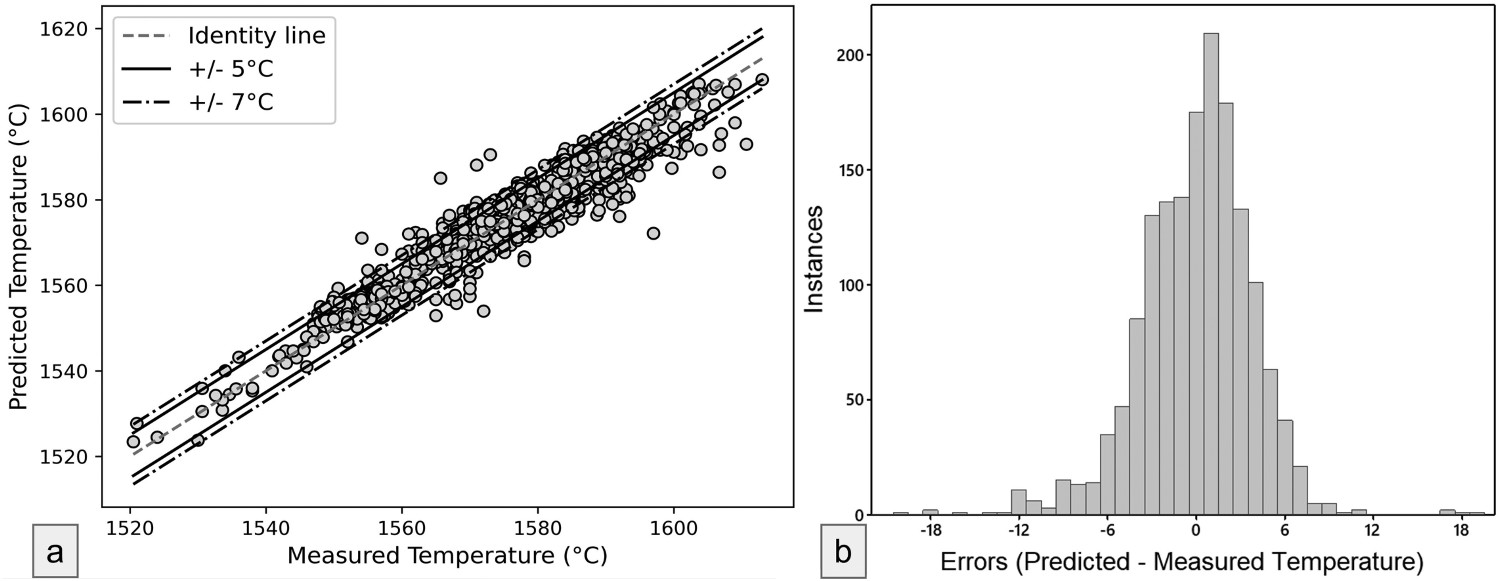

The LRF model’s parameters were optimised for maximum regression accuracy using the grid search method. The optimised parameters values are shown in Table 4. Twenty-five random forests were fitted at a learning rate of 10%, indicating that the model performs better with a slow learning approach, as suggested by James et al. [23]. Furthermore, the optimal values for the parameters related to random forest show that the model performs better with relatively simple tree structures, which is also indicative of the strength of the slow learning approach.

OPEN IN VIEWER

Table 4.

LRF model’s optimal parameters.

Parameter	Value
RF number of estimators	150
RF minimum sample split	2
RF minimum sample leaf	4
RF maximum features	$\sqrt {{\rm number\; of\; features}}$ number of features
RF maximum depth	10
RF maximum leaf nodes	10
LRF boosting estimators	25
LRF learning rate	0.1

A comprehensive analysis was conducted to reveal each variable's importance to the regression models. The variables were evaluated using their p-value and the linear coefficient for the MLR. The permutation importance analysis was employed for the RF and the LRF regressions.

Table 5 shows the resulting p-value for each variable. Most of the chosen variables are statistically significant for the MLR. The variables time of tundish pre-heating and ladle furnace power on time resulted in a p-value greater than 0.05, which means that they are not statistically significant for the MLR.

OPEN IN VIEWER

Table 5.

P-value for the model’s variables.

Variable	p-value
Coefficient	0.000
Casting superheat	0.000
Waiting period	0.000
Batch order in the casting sequence – 1	0.000
Batch order in the casting sequence – 2
Batch order in the casting sequence – 3
Batch order in the casting sequence – >4
Ladle preheating time – 1hr	0.000
Ladle preheating time – 2hr
Ladle preheating time – 4hr
Ladle preheating time – >4hr
Ladle cycle – <70min
Ladle cycle – <85min
Ladle cycle – <100min
Ladle cycle – >100min
Casting duration	0.000
Residence time	0.000
Ladle skull	0.000
Ladle life	0.010
Number of strands	0.014
Tundish preheating time	0.121
LF poweron time	0.755

When the input data is normalised, the linear regression coefficient can measure the variable's importance: the larger the coefficient, the more significant the variable is for the regression. Figure 6 shows the linear regression coefficients for each variable used to train the model.OPEN IN VIEWER

Figure 6.

Linear regression coefficients for normalised data.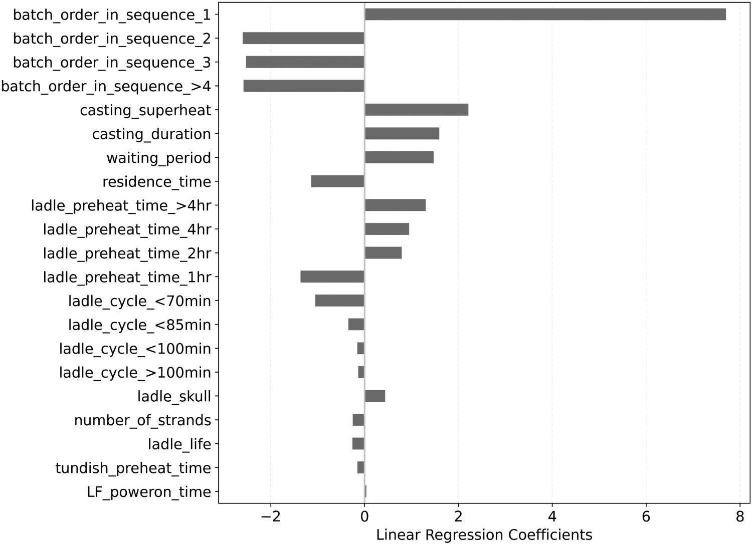

The batch order in the casting sequence was considered a categorical input and divided into four groups: first, second, third, and all subsequent batches after the third. The variable for the first batch in the sequence order has the largest coefficient. This result is expected due to the greater thermal loss of the steel to the tundish refractory walls in the first heat. As the casting continues, tundish walls become progressively hotter, and this thermal loss is reduced. Therefore, there is no significant difference between the coefficients from the second, third, and fourth heats onwards.

The variable with the second highest coefficient is the casting superheat. The last temperature in secondary refining must increase to increase the casting superheat, so this result is foreseen. The casting duration is the third most influential variable. Considering an approximately constant thermal loss in the tundish, the longer the casting time, the higher the temperature required to maintain the same average casting superheat. The waiting period between secondary refining and casting has the fourth highest coefficient, which is explained by the direct correlation between the waiting period duration and the thermal losses in that stage.

The steel residence time on the ladle and the ladle cycle or pre-heating time are also significant to the model since they represent the ladle's thermal history, which strongly affects steel temperature losses. The residence time has a negative coefficient, which is consistent with the literature, because as the time the ladle stays in contact with molten steel increases, the hotter its refractory walls become, reducing steel thermal losses to the ladle’s walls.

The ladle cycle quantifies the time the ladle stays without steel between heats, and the ladle refractory wall’s heat loss to the environment is larger as the time in this stage increases. Figure 6 shows that the shorter the ladle cycle, the greater its negative coefficient in the regression. This result is expected because the steel heat loss for the ladle is reduced with a shorter ladle cycle, so a smaller secondary refining end temperature is required.

In the plant’s operation practice, the ladle’s pre-heating duration increases with the time the ladle stays without molten steel, which is consistent with the increase in its linear coefficient as the pre-heating time increases since the ladle’s walls become cooler. Ladles that only pre-heat for one hour started their pre-heating process with less than 100 min cycle. This group presented a greater negative coefficient and thus a lower steel temperature loss to the ladle, compared to ladles with less than 70 min cycle. This result may be due to a lower heat loss from the ladle's walls to the environment since the ladle is covered during the pre-heating process and uncovered during waiting periods.

Despite being statistically significant to the MLR, the quantity of skull in the ladle, the ladle life, and the number of strands have a low coefficient in the regression. The tundish pre-heating time and the ladle furnace power on time have the lowest coefficients, which is consistent with their p-value, as they are not statistically relevant to the MLR.

The random forest regression’s permutation importance analysis was also performed. Figure 7 shows that most of the chosen variables are likewise relevant to the model. The most significant variables are the batch order in the casting sequence, the casting superheat, the waiting period, and the casting duration, which are also the variables with the highest coefficient in the linear regression model. However, a remarkable difference between the analysis is that some variables that were not statistically relevant for the MLR are meaningful for the RF regression, such as the ladle furnace power on time and the tundish pre-heating time. This indicates the presence of non-linear relationships in the dataset and that the models can potentially complement each other for better performance.OPEN IN VIEWER

Figure 7.

RF permutation importance.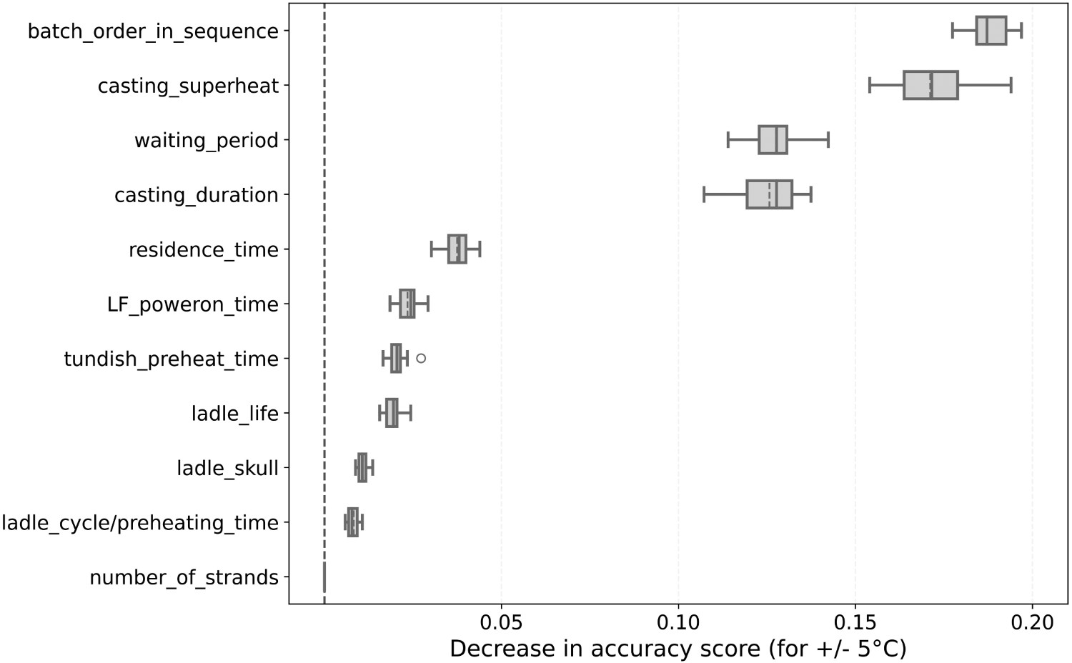

Figure 8 shows the results of the permutation importance analysis for the LRF model. The two most relevant variables for the model are the casting superheat and the order of the batch in the casting sequence, which are also the most relevant variables for both MLR and RF models. Comparing the permutation importance analysis of the RF and the LRF models, some variables that were not relevant for the RF model became more significant for the LRF, such as the ladle cycle and pre-heating time. It is widely acknowledged in the literature that these variables are significant for understanding steel thermal losses in a steelmaking plant. Therefore, the models complement each other for better performance.OPEN IN VIEWER

Figure 8.

Permutation importance for the LRF model.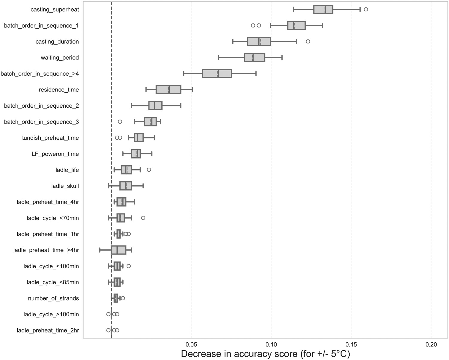

Conclusions

In this work, a hybrid statistical approach based on multiple linear and random forest regression to predict the end molten steel temperature at the secondary refining was proposed and evaluated. The proposed hybrid method first applies multiple linear regression to model the linear relationships in the dataset, then applies multiple iterations of random forest regression to improve accuracy by accounting for non-linear relationships. The two regression methods were combined using a boosting ensemble technique, in which the models are fitted sequentially using the previous model's residuals. The performance of the models was evaluated on industrial data using the RMSE metric and the accuracy to a fixed threshold.

The variables included in the models were chosen based on the literature review and validated using the p-value in the linear regression and permutation feature importance analysis for the RF and LRF regressions. The most significant variables were the batch order in the casting sequence, the casting superheat, the waiting period, the casting duration, and the residence time.

The proposed hybrid method outperformed both the linear and random forest regression methods individually. The LRF method achieved 85.3% accuracy within a range of ±5°C and 94.5% accuracy within a range of ±7°C, which is up to 5% better accuracy compared to each method alone. The accuracy of the developed method was found to be suitable for application in the industry to improve the temperature control of molten steel in continuous casting.

Footnotes

Acknowledgements

The authors are grateful to Gerdau Ouro Branco for kindly providing the industrial data for this study. They are also thankful to Redemat, Universidade Federal de Ouro Preto, CNPq and FAPEMIG for all their support.

Disclosure statement

No potential conflict of interest was reported by the authors.

References

1.

World Steel Association . (2022). 2022 world steel in figures. World Steel Association. https://worldsteel.org/steel-topics/statistics/world-steel-in-figures-2022/.

Go to Reference

2.

Chakraborty S , Sahai Y. Effect of slag cover on heat loss and liquid steel flow in ladles before and during teeming to a continuous casting tundish. Metall Trans B. 1992;23:135–151.

+ Show References

3.

Garcia A. Solidificação: fundamentos e aplicações. Campinas: Editora da UNICAMP; 2007.

Go to Reference

4.

Brimacombe JK , Sorimachi K. Crack formation in the continuous casting of steel. Metall Trans B. 1977;8:489–505.

Go to Reference

5.

Huang X , Thomas BG , Najjar FM. Modeling superheat removal during continuous casting of steel slabs. Metall Mater Trans B. 1992;23:339–356.

Go to Reference

6.

Gupta N , Chandra S. Temperature prediction model for controlling casting superheat temperature. ISIJ Int. 2004;44:1517–1526.

+ Show References

7.

Sonoda S , Murata N , Hino H , et al.A statistical model for predicting the liquid steel temperature in ladle and tundish by bootstrap filter. ISIJ Int. 2012;52:1086–1091.

Go to Reference

8.

Jormalainen T , Louhenkilpi S. A model for predicting the melt temperature in the ladle and in the tundish as a function of operating parameters during continuous casting. Steel Res Int. 2006;77:472–484.

Go to Reference

9.

Tian H , Mao Z , Wang A. A new incremental learning modeling method based on multiple models for temperature prediction of molten steel in LF. ISIJ Int. 2009;49:58–63.

Go to Reference

10.

WANG Y-n , Bao Y-p , Cui H , et al.Final temperature prediction model of molten steel in RH-TOP refining process for IF steel production. J Iron steel Res, Int. 2012;19(3):1–5.

Go to Reference

11.

He F , Dong-feng HE , An-jun XU , et al.Hybrid model of molten steel temperature prediction based on ladle heat status and artificial neural network. J Iron Steel Res Int. 2014;21, n. 2:181–190.

Go to Reference

12.

Sousa SIV , Martins F , Alvimferraz M , et al.Multiple linear regression and artificial neural networks based on principal components to predict ozone concentrations. Env Mod Softw. 2007;22:97–103.

Go to Reference

13.

AL-ALAWI SM , Abdul-wahab SA; , Bakheit CS. Combining principal component regression and artificial neural networks for more accurate predictions of ground-level ozone. Environ Model Softw. 2008;23:396–403.

Go to Reference

14.

Adusumilli S , Bhatt D , Wang H , et al.A novel hybrid approach utilizing principal component regression and random forest regression to bridge the period of GPS outages. Neurocomputing. 2015;166:185–192.

Go to Reference

15.

Shearer C. The CRISP-DM model: the new blueprint for data mining. J. Data Warehous. 2000;5, (4):13–22.

Go to Reference

16.

Breiman L. Random forests. Mach Learn. 2001;45:5–32.

+ Show References

17.

Hancock JT , Khoshgoftaar TM. Survey on categorical data for neural networks. J Big Data. 2020;7(1):1–41.

Go to Reference

18.

Lantz B. Machine learning with R: expert techniques for predictive modeling. Packt publishing ltd; 2019.

Go to Reference

19.

Potdar K , Pardawala TS , Pai CD. A comparative study of categorical variable encoding techniques for neural network classifiers. Int J Comput Appl. 2017;175:7–9.

Go to Reference

20.

Pedregosa F , et al.Scikit-learn: machine learning in python. J Mach Learn Res. 2011;12:2825–2830.

+ Show References

21.

Abraham A , Pedregosa F , Eickenberg M , et al.Machine learning for neuroimaging with scikit-learn. Front Neuroinform. 2014;8:14–14.

Go to Reference

22.

Montgomery DC. Introduction to statistical quality control. Arizona State University: John Wiley & Sons; 2007.

Go to Reference

23.

James G , Witten D , Hastie T , et al.An introduction to statistical learning. New York: springer; 2013.

+ Show References

24.

Kingsford C , Salzberg SL. What are decision trees?Nat Biotechnol2008;26:1011–1013.

Go to Reference

25.

Hastie T , Tibshirani R , Friedman J. The elements of statistical learning: data mining, inference, and prediction. New York: springer; 2009.

Go to Reference

26.

Chen X , Ishwaran H. Random forests for genomic data analysis. Genomics. 2012;99:323–329.

Go to Reference

27.

Bishop CM , Nasrabadi NM. Pattern recognition and machine learning. New York: springer; 2006.

Go to Reference

28.

Liashchynskyi P , Liashchynskyi P. Grid search, random search, genetic algorithm: a big comparison for NAS. arXiv preprint arXiv:1912.06059, 2019.

Go to Reference