Multivariate image analysis of realgar–orpiment flotation froths

Abstract

Multivariate image analysis was used to estimate the arsenic concentrations in froths resulting from the flotation of different mixtures of realgar and orpiment particles in a laboratory batch flotation cell. The realgar floated rapidly and in excess of 90% of the mineral could be recovered after 2 minutes, whereas only 48–75% of the orpiment could be recovered in the same time. Textural features, based on grey level co-occurrence matrices (GLCMs), local binary patterns (LBPs), steearable pyramids and textons were used in the analysis. Random forest models could explain approximately 71–77% of the variance in the arsenic using either of the texton, steerable pyramid or LBP features. This was considerably better than what could be obtained with the GLCM features. Monitoring of froth flotation cells was simulated with the batch data. The texton textural features were the most discriminatory with regard to detecting changes in the arsenic content of the froth.

Keywords

Multivariate image analysis froth flotation arsenic texture random forests

Introduction

Although mineral grade is a key indicator of performance in flotation systems, its online measurement is challenging, and in turn this is an impediment to the development of advanced process control systems in flotation. Real-time grade information can be obtained by the use of X-ray on-stream analysers, but these devices are expensive, and can have long sampling times, with limited accuracy (Del Villar et al. 2010). In principle, these difficulties can be circumvented by the use of froth image analysis (Duchesne 2010), and several studies have indicated that the concentrate grade of a froth flotation system can be inferred from the spectral and textural features extracted from froth images (Moolman et al. 1995; Bonifazi et al. 2000; Kaartinen et al. 2006; Aldrich et al. 2010). Recent studies related to grade estimation in froth systems comprise the platinum group metals (Marais & Aldrich 2011), base metals (Jahedsaravani et al. 2014), coal (Tan et al. 2016; Zhang et al. 2016), antimony (Liu et al. 2015; Wu et al. 2015), bauxite (Cao et al. 2013; Gui et al. 2013) and a number of others. In this study, estimation of grades is extended to arseniferous froths.

Moreover, in addition to feasture extraction based on grey level co-occurrence matrices (GLCMs) that have been used in froth texture analysis for more than two decades, three algorithms relatively new in mineral processing, viz. local binary patterns (LBPs), steerable pyramids and textons are considered. Despite their successful application in other technical disciplines, these methods have not been used in froth image analysis to any significant extent as yet.

To this end, a realgar (A₂S)–orpiment (A₂S₃) system with a quartz diluent was investigated. These arsenic sulphides are present as gangue materials in base metal flotation, especially copper and nickel systems (Smith et al. 2013), where their removal is problematic (Smith et al. 2012). Since arsenic is a penalty element for base metal smelters (Ma & Bruckard 2009; Haque et al. 2012), an online system for detecting arsenic in froth concentrate, such as considered in this paper, could be of considerable commercial benefit.

Experimental methodology

Mineral preparation

The realgar and orpiment samples were obtained from the Palomo Mine in Julcani Province, Peru. Hand-sorted samples were stage-crushed manually using a ceramic mortar and pestle, to pass 10 mesh (1.65 mm). Fines were removed from the crushed material by screening at 212 µm. Locally obtained and prepared quartz of a high quality was used as the gangue mineral in the flotation tests. Four-hundred and seventy five g of −1650 + 212 µm quartz was used in each test and the combined mass of the individual flotation charges, i.e. realgar and/or orpiment plus quartz diluent, was 500 g. For all flotation tests, the realgar, orpiment and quartz were ground in a stainless steel mill at the natural pH using distilled water at 67% solids by weight.

Flotation equipment

The arsenic sulphide samples were floated in a 3 dm³ stainless steel-modified Denver cell, with a bottom-driven, variable speed impeller. As shown in Figure 1, the whole surface of the froth could, therefore, be scraped with a paddle at a constant depth and rate.

Figure 1

Laboratory batch flotation cell.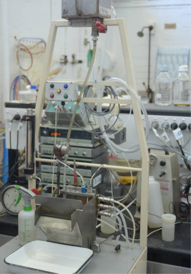

A combined electrode was used to measure the pH continuously during testing. Likewise, a high impedance, differential voltmeter was used to continuously measure the pulp potential during testing. The voltmeter was equipped with a polished platinum flag electrode and an Ag/AgCl reference electrode. To set and maintain the pulp pH, acid and base could be added automatically with radiometer TTT80 titrators and ABU80 burettes.

The impeller speed was set at 1200 rpm for both conditioning and flotation. During flotation, frother was added continually with a motorised variable speed dispenser, starting 1 min before flotation. The flotation gas consisted of high-purity synthetic air, flowing at 8 dm³min⁻¹. The frother addition rate was set to maintain a high active froth column that would not limit flotation rates and which was similar to rougher flotation in practice. Froth images were captured by a Nikon D7000 SLR camera used in video mode at 24 frames/s. The camera was fitted with a Nikon AF Nikkor, 28–105 mm, 1:3.5-4.5D lens and was mounted on a tripod.

Experimental procedure

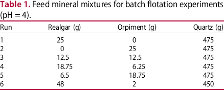
Flotation experiments with the mineral–quartz mixtures were conducted according to a standard procedure developed by CSIRO. Once the ground pulp was transferred to the flotation cell, the water level was raised to a preset level and the pH was adjusted to the test value. Concentrates were collected after approximately 0.5, 1, 2, 4 and 8 min. Six batch runs with different mineral mixtures, each totalling 500 g, were conducted, as summarised in Table 1. Images associated with the froths of each run are shown in Figure 2.

Figure 2

Realgar–orpiment froth image data set collected from batch runs listed in Table 1, showing Runs 1–6 from top to bottom, respectively. Each row shows five bursts of three images each, from left to right, collected at approximately 0.5, 1, 2, 4 and 8 minutes, respectively.

Table 1

Feed mineral mixtures for batch flotation experiments (pH = 4).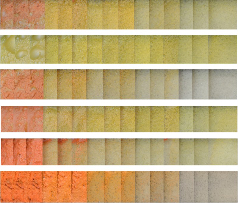

Run	Realgar (g)	Orpiment (g)	Quartz (g)
1	25	0	475
2	0	25	475
3	12.5	12.5	475
4	18.75	6.25	475
5	6.5	18.75	475
6	48	2	450

Multivariate image analysis

Features were extracted from the digital images of the froths by means of red–green–blue (RGB) colour analysis and four textural feature extraction methods, based on the use of GLCMs, wavelets, LBPs and textons. The RGB features of each image were simply the mean red, green and blue intensities of the images. The other approaches are briefly summarised below. After the features were extracted, regression with random forest models was applied to relate the froth features to the arsenic content of the froths.

Grey level co-occurrence matrices

Consider a GLCM of an image I to be denoted as , where d is a chosen displacement between each pair of pixels and G is the number of grey levels in in the image. Each entry of the sized GLCM is the number of times that the grey level pair occurs at a displacement of exactly d in , as indicated in Figure 3.

Figure 3

A co-occurrence matrix shows the frequency of every particular pair of grey levels in pixel pairs, separated by a certain distance d along a certain direction a or equivalently as specified by Cartesian coordinates.

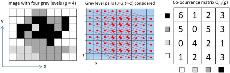
Natural greyscale images most commonly still consist of 8-bit images with 2⁸= 256 pixel intensities or grey levels (each grey level g is, therefore, in the range ). However, in GLCM calculations, fewer grey levels (G) are often used to reduce computation time and noise in the image.

Finally, GLCMs are normalised, so that their elements sum to unity, which means that the GLCM becomes a probability matrix of joint pixel occurrences. In this study, eight GLCM features, as defined by Haralick et al. (1973), were generated by calculating the mean values and standard deviations of the energy, , contrast, , correlation, and homogeneity, over four different orientations 0°, 45°, 90° and 135°, where represents the entry in row i and column j of the normalised GLCM , while and are respectively the mean and standard deviation of the ith row of the GLCM, and and are the mean and standard deviation of the jth column of the GLCM.

Steerable pyramids

Steerable pyramids are multiscale image representations that are obtained by convolving an image with several two-dimensional oriented band-pass filters, as well as high-pass and low-pass filters. This is different from wavelet representations that are obtained by convolving the image horizontally and vertically with one-dimensional functions derived from a mother wavelet. The special design of the filter bank makes the steerable pyramid representation both translation and rotation invariant. Steerable pyramids were developed in the 1990s to counter the limitations of orthogonal separable wavelet decompositions that had become popular in image processing in the late 1980s (Simoncelli et al. 1992; Simoncelli & Freeman 1995).

Their basis functions are kth order directional derivative operators in different sizes and k + 1 orientations that allow linear multi-scale, multi-orientation image decomposition. On this basis, they span a rotation- and translation-invariant subspace. Steerable pyramids have been applied in a diverse range of problems, such as texture classification (Greenspan et al. 1994; Do & Vetterli 2002; Li & Shawe-Taylor 2005) and texture synthesis (Heeger & Bergen 1995; Portilla & Simoncelli 2000), but not much in mineral processing yet.

A block diagram for the decomposition is shown in Figure 4. To start with, the image is separated into low- and high-pass subbands by the use of filters L₀ and H₀. This is followed by dividing the low-pass subband into a set of oriented band-pass subbands and a lower pass subband that is subsampled by a factor of 2 in a horizontal and vertical direction. The recursive construction of a pyramid is obtained by inserting a copy of the portion of the diagram delineated with a broken line at the location of the solid circle.

Figure 4

Decomposition of images with steerable pyramids.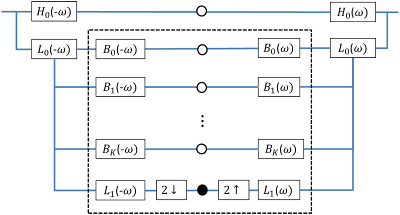

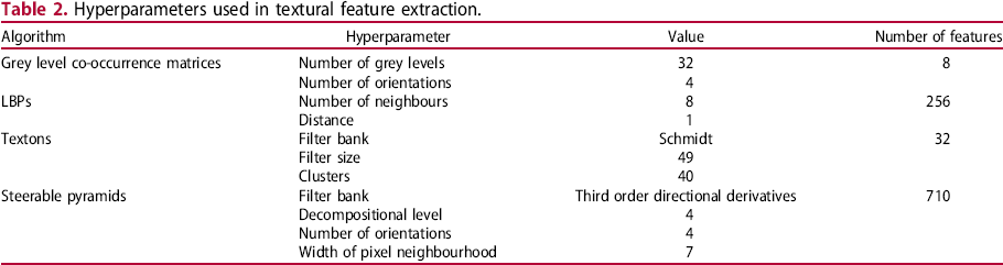
Different groups of statistical descriptors can be extracted, such as marginal statistics, correlation coefficients, magnitude correlations and cross-scale phase statistics. The resultant feature sets are large, but dimensionality reduction methods, such as principal component analysis or feature selection techniques may be used to reduce the size of the feature set. The hyperparameters that were used in this investigation are summarised in Table 2.

Table 2

Hyperparameters used in textural feature extraction.

Algorithm	Hyperparameter	Value	Number of features
Grey level co-occurrence matrices	Number of grey levels	32	8
Grey level co-occurrence matrices	Number of orientations	4	8
LBPs	Number of neighbours	8	256
LBPs	Distance	1	256
Textons	Filter bank	Schmidt	32
	Filter size	49
	Clusters	40
Steerable pyramids	Filter bank	Third order directional derivatives	710
	Decompositional level	4
	Number of orientations	4
	Width of pixel neighbourhood	7

Local binary pattern operators

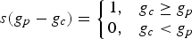
Local binary pattern operators are applied to greyscale images on a pixel-by-pixel basis by comparing the intensity of each pixel to those of the eight other pixels in its immediate neighbourhood (Ojala et al. 1994). A binary thresholding function s is applied to the difference in the intensity between each neighbouring pixel and the centre pixel under consideration : 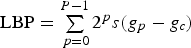(1) As shown in Figure 5, the resultant LBP is subsequently computed as . By applying the LBP operator to each pixel in an image with G grey levels, the image is represented by LBPs ranging from 0 to G. This will be referred to as the LBP image. Unlike feature extraction by the use of GLCMs, the number of grey scales in natural images is not usually reduced prior to calculations, so that when the frequency histogram of the LBP image is computed, it would yield a larger number of features (e.g. 256 features for 8-bit images) to be used in the subsequent classification step.

Figure 5

Example of (a) a centre pixel (shaded grey), with its eight neighbouring pixels (the numbers represent arbitrary pixel intensities), (b) the values obtained through thresholding and (c) the weights by which the thresholded values are multiplied to give the decimal LBP value (shown in place of the centre pixel).

LBP feature extraction has been applied with considerable success in many fields, including remote sensing (Vatsavai et al. 2010), face recognition (Ahonen et al. 2006) and biomedicine (Nanni et al. 2012), but has only recently been considered in mineral processing (Kistner et al. 2013; Aldrich et al. 2014, 2015; Fu & Aldrich 2016).

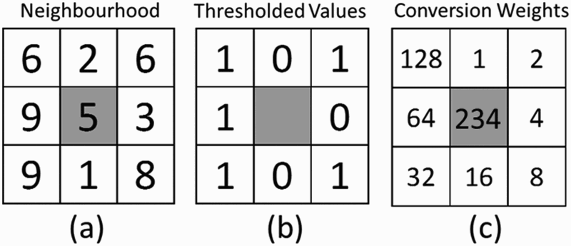
Textons

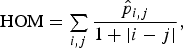
Textons can be defined as cluster centres in a filter response space that are computed through convolution of a training set of images with oriented linear spatial basis functions arranged in a filter bank (Leung & Malik 2001), as indicated diagrammatically in Figure 6. Each pixel in an image is mapped to a feature space, the dimensionality of which is determined by the filter set being used, while the cluster centres in the filter response space can be determined by any suitable clustering method. These cluster centres are referred to as the texton dictionary and the values of a texton feature associated with an image consist of a count of the number of pixels assigned to the specific texton channel (Kistner et al. 2013).

Figure 6

Extraction of texton feature vectors from images.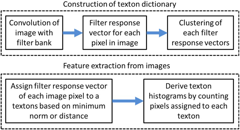

The Schmidt filter bank used in this investigation comprises 13 rotationally invariant filters of the form described in eq. (2), (2) where r represents the pixel coordinates in the image, is the scale and is the frequency or number of cycles in the Gaussian envelope of the filter (Varma & Zisserman 2005).

Although the analysis of texture in the context of ore sorting, bulk solids characterisation (Jemwa & Aldrich 2012) and froth image analysis (Kistner et al. 2013) is well established in the mineral processing literature, the use of textons has not figured prominently in these studies as yet.

Random forest model

A random forest (Breiman 2001) is an ensemble of K classification or regression trees that are constructed not only by using different bootstrapped training sets for each tree, but also by restricting the available split variables at each node to randomly drawn input variables (Breiman 2001), as summarised below (Aldrich & Auret 2013):

For k = 1 to K (size of ensemble)

Construct a bootstrap sample with replacement X ^k from the learning set X, of the same size as the learning set

Grow a random forest tree t_k on X ^k by employing the CART tree growing algorithm, with the following modification at each node:

i. Select random input variables from X ^k to use as possible split variables

ii. Calculate best split position ς* from these variables

iii. Split the node into two child nodes

Repeat the above tree growing algorithm until the following stopping criteria are achieved:

i. A node size of one (for classification) or five (for regression)

ii. A node with homogenous class membership or response values

Output the ensemble of trees T = {t_k}₁^K

A new prediction is made as follows:

The prediction of each tree t_k(x) is calculated

For classification, the majority vote over all K trees is assigned

For regression, the average response value over all K trees is assigned

Random forests have been applied extensively in many technical fields, since they were first proposed by Breiman. They are also slowly finding their way into the mineral processing and geosciences literature (e.g. Auret & Aldrich 2011, 2012; O'Brien et al. 2015; Rodriguez-Galiano et al. 2015).

Results and Discussion

Mineral recovery

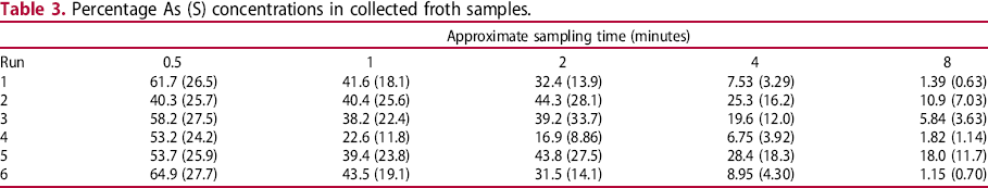
The recoveries of realgar, orpiment, quartz and water during the batch runs summarised in Table 1 are shown in Figure 7. In general, in excess of 95% of the realgar was recovered within 2 minutes, followed by full recovery after 8 minutes, when the runs were terminated. Orpiment, on the other hand, floated more slowly and recovery was not fully complete after 8 minutes. In addition to Figure 7, the As concentrations measured during each run are summarised in Table 3.

Figure 7

Recovery of minerals in batch runs at pH = 4: 25 g R, 475 g Q (Run 1, top left), 25 g O, 475 g Q (Run 2, top right), 12.5 g R, 12.5 g O 475 g Q (Run 3, middle left), 18.75 g R, 6.25 g O, 475 g Q (Run 4, middle right), 6.25 g R, 18.75 g O, 475 g Q (Run 5, bottom left), 48 g R, 2 g O, 475 g Q (Run 6, bottom right).

Table 3

Percentage As (S) concentrations in collected froth samples.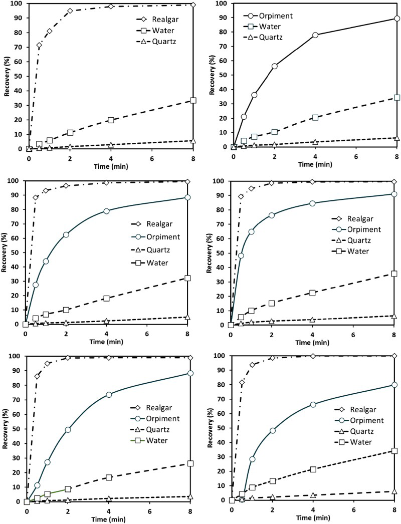

	Approximate sampling time (minutes)
Run	0.5	1	2	4	8
1	61.7 (26.5)	41.6 (18.1)	32.4 (13.9)	7.53 (3.29)	1.39 (0.63)
2	40.3 (25.7)	40.4 (25.6)	44.3 (28.1)	25.3 (16.2)	10.9 (7.03)
3	58.2 (27.5)	38.2 (22.4)	39.2 (33.7)	19.6 (12.0)	5.84 (3.63)
4	53.2 (24.2)	22.6 (11.8)	16.9 (8.86)	6.75 (3.92)	1.82 (1.14)
5	53.7 (25.9)	39.4 (23.8)	43.8 (27.5)	28.4 (18.3)	18.0 (11.7)
6	64.9 (27.7)	43.5 (19.1)	31.5 (14.1)	8.95 (4.30)	1.15 (0.70)

Prediction of as concentrations

Features were extracted from the froths, based on the use of GLCM, LBP, steerable pyramids and textons, as discussed in the previous section. This resulted in four sets of features being associated with each image, as summarised in Table 2.

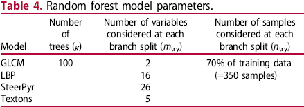
In order to estimate the arsenic concentrations from the image features, random forest models were fitted to a random sample consisting of 500 records, and tested against the remaining 85 records. The parameters used to fit the models are summarised in Table 4. The results of the models based on the independent test data sets are shown in Figure 8. The squared correlation coefficients of each of the models are also shown in the figure. Although there are small differences in the nominal R² values of the models fitted with the LBP, steerable pyramid and texton predictors, these differences are not statistically significant. However, the model fitted with the GLCM features did not perform as well as than the other three models (at a 95% confidence level).

Figure 8

Prediction of the %As in the froths by the use of the random forest regression models. The model fits on independent test sets are indicated by the R² values in parentheses.

Table 4

Random forest model parameters.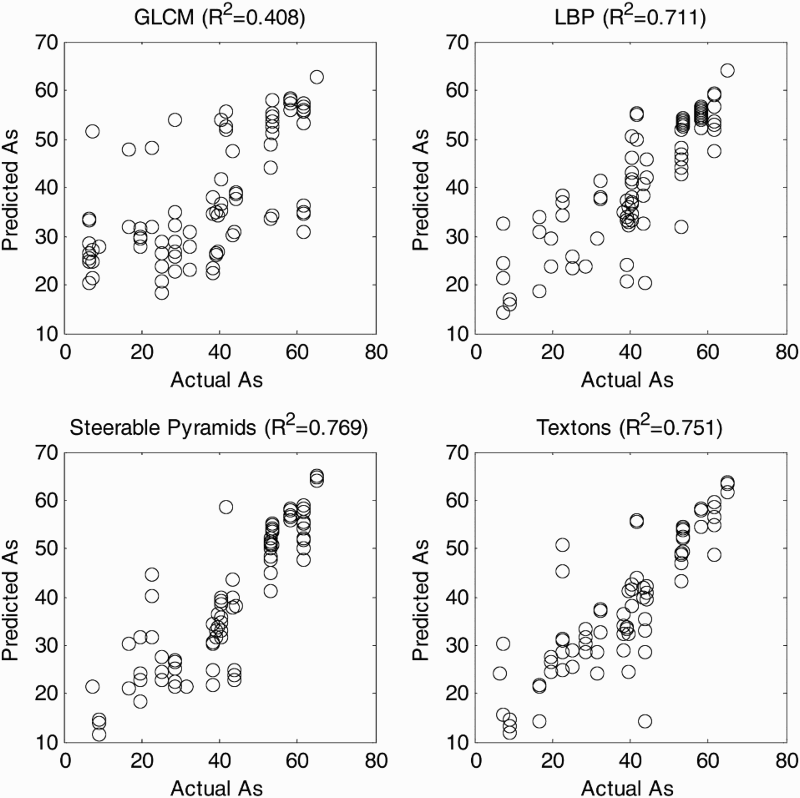

Model	Number of trees ( _K )	Number of variables considered at each branch split (m_try)	Number of samples considered at each branch split (n_try)
GLCM	100	2	70% of training data (=350 samples)
LBP		16
SteerPyr		26
Textons		5

Monitoring of froth flotation systems by the use of image features

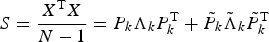
Online monitoring of the performance of the flotation cell based on the froth image variables can be done in a multivariate statistical process control framework. This entails the construction of a principal component model of the variables and the derivation of diagnostic indices with appropriate control limits to enable automatic fault detection. Fault diagnosis would be more complicated, since the froth image variables do not have physical meaning. However, in principle, it should still be possible to steer the process back to normal conditions in case of deviation, as outlined more formally below.

Monitoring scheme

Consider the froth image variable set to be denoted by comprising M variables and N measurements. Then is the covariance matrix of the image variables, typically scaled to zero mean and unit variance, is the loading matrix of the first k < M principal components, is a diagonal matrix containing the k eigenvalues of the decomposition, is the loading matrix of the M − k remaining principal components and 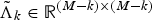is a diagonal matrix containing the M − k remaining eigenvalues of the decomposition. is an M × M identity matrix, while matrices and can be expressed in terms of the loading and diagonal matrices of the model. (3) (4) (5)

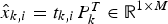
Only the and -statistics derived from Equations (4) and (5) are monitored and not the original variables. The - or -statistic is an indication of the distance of the ith measurement vector from the centre of the principal component plane, while the squared prediction error or -statistic represents the model error. The principal component score vectors are calculated by projecting the measurement vectors onto the loading matrix, i.e. . Conversely, the measurement vectors can be approximated by .

The control limits for the and -statistics, or projection of the variables to a latent variable space or score map, were derived by means of kernel density estimation.

Simulated case study: Runs 1 and 3

For the case study, steady-state conditions were simulated from the batch data from Runs 1 and 3 by considering the flotation after 30 seconds in each batch experiment, just before the collection of the first sample. Forty images were collected from each batch around these points and LBP features were extracted. The texture neighbourhood and sampling point pair (R, P) were (4, 16) and the mapping was both rotationally invariant and uniform (Kistner et al. 2013). This yielded 192 features, to which a principal component model was fitted, as summarised by Equations (3)–(5). The first 15 eigenvalues of the model are shown in Figure 9.

Figure 9

First 15 eigenvalues of the principal component model.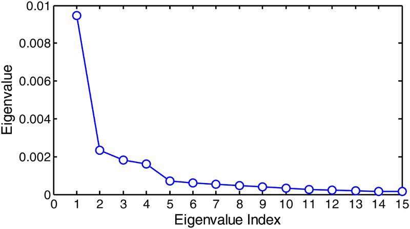

Eight components collectively explaining 87.0% of the variance in the LBP features were retained. With this model, the and Q_i-statistics were calculated for the data representing normal operating conditions (Run 1). The principal component scores of the new data (Run 3, simulated fault condition) were calculated by projecting onto the principal component model.

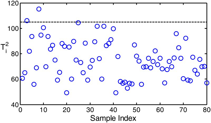
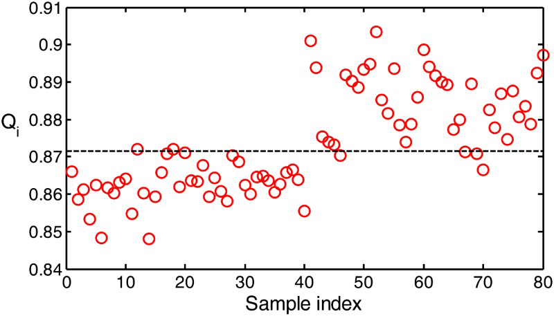
These results are shown in Figures 10 and 11. In these figures, the samples with indices from 1 to 40 were collected from the simulated normal operating conditions and those with indices from 41 to 80 were representative of the fault condition. As can be seen from Figure 10, the chart did not indicate a fault condition (almost zero samples above the broken line or 95% control limit). However, the fault condition was clearly identified in Figure 11, where 90% of the samples exceeded the control limit.

Figure 10

T²-statistics for the simulated normal operating conditions based on image data associated with the first sampling point in Run 1 (sample index 1–40) and simulated fault condition based on image data associated with the first sampling point in Run 3 (sample index 41–80). The broken line represents the 95% control limit.

Figure 11

Q-statistics for the simulated normal operating conditions based on image data associated with the first sampling point in Run 1 (sample index 1–40) and simulated fault condition conditions based on image data associated with the first sampling point in Run 3 (sample index 41–80). The broken line represents the 95% control limit.

Simulated case study: Runs 3 and 4

In the second case study, the 35 texton features extracted from images associated with Run 3 were used as variables for online monitoring of the performance of the flotation system after 30 seconds. A principal component model was fitted to 50 samples (images) from batch 1, simulating normal operating conditions. The first four principal components could explain 80.2% of the variance in the texton features. Thirty samples collected after 30 s in Batch Run 4 were projected onto the first eight principal components.

In Figure 12, normal operating conditions, based on image data associated with the first sampling point in Run 3, are indicated by the circular markers and the simulated process deviations, based on image data associated with the first sampling point in Run 4, are indicated by the star markers. The broken line represents the 95% control limit. This decision boundary was fitted to the normal data by means of a Gaussian mixture model containing five components. The froth images in the graph have a similar appearance, as indicated by two examples of the froth images on the right in the figure, and the differences may not be readily observed by an inexperienced operator. Despite this, the first two principal components, collectively explaining approximately 63% of the variance in the 35 texton features, could be used to reliably discriminate between the images.

Figure 12

Principal component score plot of texton features extracted from froth images collected after 30 s from Batch Runs 3 (top image, star markers) and 4 (bottom image, circular markers).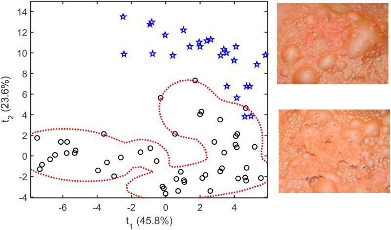

Conclusions

From this investigation, where the use of froth image analysis to estimate arsenic concentration in the realgar–orpiment batch flotation froth system was investigated, the following can be concluded:

During batch flotation, the realgar could be recovered faster and more completely (approximately 99% after 8 minutes) than the orpiment (approximately 90% after 8 minutes).

For flotation of realgar–orpiment ores, grades could be estimated from features extracted from froth images based on textural features extracted with different algorithms.

Random forest regression models could explain up to 77% of the variance in the arsenic concentration when texton features served as predictor variables. This was better than what could be achieved when GLCM features were used, but similar to what could be achieved with LBP and steerable pyramid features.

As a consequence, these features could be used as variables in a multivariate statistical process monitoring framework for online monitoring of the concentration grade in the flotation system.

This demonstrates potential for further industrial development of this important application, given that the quality of advanced (model-based) control systems crucially depends on the quality of the underlying models.

Footnotes

Acknowledgement

The authors are grateful for financial support for the project provided by the National Research Foundation in South Africa.

Disclosure statement

No potential conflict of interest was reported by the authors.

References

Ahonen

, Hadid

, Pietikäinen

2006. Face description with local binary patterns: application to face recognition. IEEE Trans Pattern Anal Mach Intell. 28:2037–2041. doi: 10.1109/TPAMI.2006.244

Aldrich

, Auret

2013. Unsupervised process monitoring and fault diagnosis with machine learning methods. London: Springer.

Aldrich

, Marais

, Shean

, Cilliers

JJ.

2010. Online monitoring and control of froth flotation systems with machine vision: a review. Int J Miner Process. 96:1–13. doi: 10.1016/j.minpro.2010.04.005

Aldrich

, Smith

, Verrelli

, Bruckhard

, Kistner

, Auret

2014. Multivariate image analysis of a realgar–orpiment batch froth flotation system. Proceedings of the 27th International Minerals Processing Congress (IMPC 2014); Oct 20–24; Chapter 4, 14–22, Santiago, Chile.

Aldrich

, Uahengo

FDL

, Kistner

2015. Particle size estimation in hydrocyclone underflow streams by use of multivariate image analysis. Miner Eng. 70:14–19. doi: 10.1016/j.mineng.2014.08.018

Auret

, Aldrich

2011. Empirical comparison of tree ensemble variable importance measures. Chemometr Intell Lab Syst. 105:157–170. doi: 10.1016/j.chemolab.2010.12.004

Auret

, Aldrich

2012. Interpretation of nonlinear relationships between process variables by use of random forests. Miner Eng. 35:27–42. doi: 10.1016/j.mineng.2012.05.008

Bonifazi

, Massacci

, Meloni

2000. Prediction of complex sulfide flotation performances by a combined 3D fractal and colour analysis of the froths. Miner Eng. 13:737–746. doi: 10.1016/S0892-6875(00)00058-3

Breiman

2001. Random forests. Mach Learn. 45:5–32. doi: 10.1023/A:1010933404324

10.

Cao

, Xie

, Gui

, Wei

, Yang

2013. Integrated prediction model of bauxite concentrate grade based on distributed machine vision. Miner Eng. 53:31–38. doi: 10.1016/j.mineng.2013.07.003

11.

Del Villar

, Desbiens

, Maldonado

, Bouchard

2010. Automatic control of flotation columns. In: Sbárbaro

, Del Villar

, editor. Advanced control and supervision of mineral processing plants. London: Springer; 249–286.

12.

, Vetterli

2002. Rotation invariant texture characterization and retrieval using steerable wavelet-domain hidden Markov models. IEEE Trans Multimed. 4:517–527. doi: 10.1109/TMM.2002.802019

13.

Duchesne

2010. Multivariate image analysis in mineral processing. In: Sbárbaro

and Del Villar

, editors. Advanced control and supervision of mineral processing plants. London: Springer; 85–142.

14.

, Aldrich

2016. Flotation froth image analysis by use of a dynamic feature extraction algorithm. Proceedings of the 17th IFAC symposium on control, optimization and automation in mining, mineral and metal processing (MMM 2016) ; August 31–September 2; Vienna, Austria.

15.

Greenspan

, Belongie

, Goodman

, Perona

1994. Rotation invariant texture recognition using a steerable pyramid. IEEE Proceedings of the 12th IAPR International Conference on Pattern Recognition, October 9–13, Jerusalem, Israel, Vol. 2, p. 162–167.

16.

Gui

, Liu

, Yang

, Chen

, Liao

2013. Color co-occurrence matrix based froth image texture extraction for mineral flotation. Miner Eng. 46–47:60–67. doi: 10.1016/j.mineng.2013.03.024

17.

Haque

, Bruckard

WJ.

Cuevas,

2012. A techno-economic comparison of pyrometallurgical and hydrometallurgical options for treating high-arsenic copper concentrates. Proceedings of the 26th International Mineral Processing Congress (IMPC 2012); September 2012, New Delhi, India, 01908–01922.

18.

Haralick

, Shanmugam

, Dinstein

1973. Textural features for image classification. IEEE Trans Syst Man Cybernet. SMC-3:610–621. doi: 10.1109/TSMC.1973.4309314

19.

Heeger

, Bergen

JR.

1995. Pyramid-based texture analysis/synthesis. Proceedings of the 22nd Annual Conference on Computer Graphics and Interactive Techniques (SIGGRAPH ‘95), August 6–11, Los Angeles, USA, p. 229–238.

20.

Jahedsaravani

, Marhaban

, Massinaei

2014. Prediction of the metallurgical performances of a batch flotation system by image analysis and neural networks. Miner Eng. 69:137–145. doi: 10.1016/j.mineng.2014.08.003

21.

Jemwa

, Aldrich

2012. Estimating size fraction categories of coal particles on conveyor belts using image texture modeling methods. Expert Syst Appl. 39:7947–7960. doi: 10.1016/j.eswa.2012.01.104

22.

Kaartinen

, Hätönen

, Hyötyniemi

, Miettunen

2006. Machine-vision-based control of zinc flotation – a case study. Control Eng Pract. 14:1455–1466. doi: 10.1016/j.conengprac.2005.12.004

23.

Kistner

, Jemwa

, Aldrich

2013. Monitoring of mineral processing systems by using textural image analysis. Miner Eng. 52:169–177. doi: 10.1016/j.mineng.2013.05.022

24.

Leung

, Malik

2001. Representing and recognizing the visual appearance of materials using three-dimensional textons. Int J Comput Vision. 43:29–44. doi: 10.1023/A:1011126920638

25.

, Shawe-Taylor

2005. Comparison and fusion of multiresolution features for texture classification. Pattern Recogn Lett. 26:633–638. doi: 10.1016/j.patrec.2004.09.013

26.

Liu

, Tang

, Wang

, Gui

, Yang

2015. Performance recognition of antimony flotation based on multi-information fusion and extension theory. Zhongnan Daxue Xuebao (Ziran Kexue Ban)/J Cent South Univ (Science and Technology). 46:4512–4520.

27.

, Bruckard

WJ.

2009. Rejection of arsenic minerals in sulfide flotation – A literature review. Int J Miner Process. 93:89–94. doi: 10.1016/j.minpro.2009.07.003

28.

Marais

, Aldrich

2011. Estimation of platinum flotation grades from froth image data. Miner Eng. 24:433–441. doi: 10.1016/j.mineng.2010.12.006

29.

Moolman

, Aldrich

, Van Deventer

JSJ.

1995. The monitoring of froth surfaces on industrial flotation plants using connectionist image processing techniques. Miner Eng. 8:23–30. doi: 10.1016/0892-6875(94)00099-X

30.

Nanni

, Lumini

, Brahnam

2012. Survey on LBP based texture descriptors for image classification. Expert Syst Appl. 39:3634–3641. doi: 10.1016/j.eswa.2011.09.054

31.

O'Brien

, Spry

, Nettleton

, Xu

, Teale

GS.

2015. Using random forests to distinguish gahnite compositions as an exploration guide to Broken Hill-type Pb–Zn–Ag deposits in the Broken Hill domain, Australia. J Geochem Explor. 149:74–86. doi: 10.1016/j.gexplo.2014.11.010

32.

Ojala

, Pietikäinen

, Harwood

1994. Performance evaluation of texture measures with classification based on kullback discrimination of distributions. IEEE Proceedings of the 12th IAPR International Conference on Pattern Recognition, October 9–13, Jerusalem, Israel, Vol. 2, p. 582–585.

33.

Portilla

, Simoncelli

EP.

2000. A parametric texture model based on joint statistics of complex wavelet coefficients. Int J Mach Vision. 40:49–70. doi: 10.1023/A:1026553619983

34.

Rodriguez-Galiano

, Sanchez-Castillo

, Chica-Olmo

, Chica-Rivas

2015. Machine learning predictive models for mineral prospectivity: an evaluation of neural networks, random forest, regression trees and support vector machines. Ore Geol Rev. 71:804–818. doi: 10.1016/j.oregeorev.2015.01.001

35.

Simoncelli

, Freeman

WT.

1995. The steerable pyramid: a flexible architecture for multi-scale derivative computation. IEEE second International Conference on Image Processing; October; Washington DC, USA.

36.

Simoncelli

, Freeman

, Adelson

, Heeger

DJ.

1992. Shiftable multi-scale transforms. IEEE Trans Inform Theory. 38:587–607. doi: 10.1109/18.119725

37.

Smith

, Davey

KJ.

Bruckard

WJ.

2012. The use of pulp potential control to separate copper and arsenic – an overview based on selected case studies. Proceedings of the 26th International Mineral Processing Congress (IMPC 2012); September 2012; New Delhi, India, 05057–05067.

38.

Smith

, Davey

, Forbes

, Bruckard

WJ.

2013. Fundamental studies of the flotation of realgar and orpiment. Proceedings of the XV Balkan Mineral Processing Congress; June 12–16; Sozopol, Bulgaria, 1, 379–384.

39.

Tan

, Liang

, Peng

, Xie

2016. The concentrate ash content analysis of coal flotation based on froth images. Miner Eng. 92:9–20. doi: 10.1016/j.mineng.2016.02.006

40.

Varma

, Zisserman

2005. A statistical approach to texture classification from single images. Int J Comput Vision. 62:61–81. doi: 10.1007/s11263-005-4635-4

41.

Vatsavai

, Cheriyadat

, Gleason

2010. Unsupervised semantic labeling framework for identification of complex facilities in high-resolution remote sensing images. IEEE International Workshop on Spatial and Spatiotemporal Data Mining (SSTDM-10), September 13, Sydney, Australia, p. 273–280.

42.

, Xie

Y-F

, Yang

C-H

, Gui

W-H.

2015. Froth-image-features-driven control strategy for addition rates of reagents in stibnium rougher flotation. Kongzhi Lilun Yu Yingyong/Control Theory and Applications. 32:1599–1606.

43.

Zhang

, Tang

, Liu

, Tan

, Xu

2016. Recognition of flotation working conditions through froth image statistical modeling for performance monitoring. Miner Eng. 86:116–129. doi: 10.1016/j.mineng.2015.12.008