
Abstract
Owing to the complex nature of heat generation in friction stir welding, equations are required to understand the effect of process parameters and tool geometry on heat generation. In this study, simplified equations for straight tool profiles have been extended to treat tapered tool profiles for triangular, square, pentagonal and hexagonal geometries. New equations have been implemented to model heat generation in a finite element software package for welding aluminium alloy. The calculated thermal profiles agree better with experimental data than those calculated using the simplified equations. It was also demonstrated that the amount of heat generation increases with increasing number of flats on the tapered tool profile, with a hexagonal tapered tool profile generating the highest temperature.
Introduction
Friction stir welding (FSW) is classified as a solid-state welding process and was invented by The Welding Institute (Cambridge, UK). The heat generation during FSW does not cause the base material to melt [1], but it is sufficient to soften the material so that a welding zone is formed due to the stirring force [2, 3]. Therefore, the mechanisms by which heat is generated during FSW are significant factors in determining the quality of the final welded joints by predicting the effect of heat input on grain size [4-6] to avoid defects in welding [7, 8].
Heat generation in FSW results from friction and deformation [9]. The heat generation depends on the contact condition. There are two main contact conditions. The sliding condition occurs when the contact shear stress at the tool-workpiece interface is less than the shear yield strength. The sticking condition occurs when the reverse is true. The combination of these contact conditions (partial sticking/partial sliding) is also possible [10].
Bastier et al. [11] reported that plastic deformation contributes 4.4% of the total heat generated. Therefore, several investigations [12-15] have assumed that heat is only generated as a result of frictional heat.
The effect of tool geometry on heat generation during friction stir welding
Tool geometry is a significant factor in controlling the heat generated during FSW [1, 16, 17]. The majority of previous investigations have focused on the shoulder features (shoulder outer surface and shoulder end surface) because together they are responsible for more than 80% of the total heat generation [1, 10, 18-20] during FSW processes.
Published studies have reported that changing FSW probe profiles increase the total heat generation. Schmidt, Hattel [10] reported that probe generated 14% from total heat generation and 17% in a recent paper [20]. Zhang et al. [13] reported that the probe heat generation fraction differs by between 13% and 37% across a range of published FSW studies. As a result, many researchers have considered the impact of probe shape on the total heat generated. Ramanjaneyulu et al. [21] reported that the total heat generation and the peak temperature increases with increasing number of flats on the tool probe (i.e. triangular to hexagonal profile).
Recently, numerous FSW thermal models have been developed to determine the relationship between heat generation and tool profile [14, 15, 22, 23]. However, tapered polygonal profiles have not yet been considered. To address this gap, in the present work analytical models are developed, which give a complete description of the influence of the polygonal tapered probe profiles on the total heat generated. These models are implemented using COMSOL (a commercial finite element package) and compared with published results from experimentation and modelling.
Equations for heat generation
Friction stir welding can be considered as the combination of extrusion, forging and stirring processes, occurring simultaneously, which results in the generation of high temperatures and strain rates [24]. Generally, the heat generated during the FSW process was considered to be a result of the friction process between the welding tool and base metal [11], but practically, it is due to friction as well as deformation. In the present work, equations are derived to calculate the heat input and contribution at surfaces (shoulder, probe side and probe tip) for different tapered tool profiles, (triangular (TR), square (SQ), pentagonal (PEN) and hexagonal (HEX)), which are shown in Figure 1. The tool dimensions (shoulder radius (Rs) 6 mm, probe radius (Rp) 3 mm, probe height (Hp) 4.7 mm and taper angle 14°) were selected to allow validation against the practical study by Ramanjaneyulu et al. [21]. The derived equations were applied in COMSOL 5.1 to calculate the temperature evolution in FSW for the selected taper probe profiles.
Geometry of various taper tool profiles.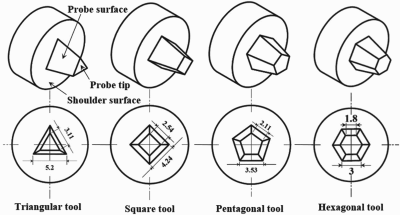
Heat generation equation for taper tools
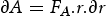
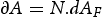
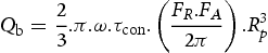
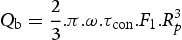
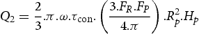
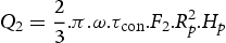
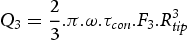
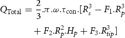
In the analytical estimation for all taper tools, a circular flat cross-section shoulder surface, a sloping trapezoidal prism probe side surface and a flat probe tip cross-section surface are assumed. The simplified tool design for the taper tools is presented in Figure 1, where Q1 is the heat generated under the tool shoulder, Q2 is the heat generated at the tool trapezoidal probe side and Q3 is the heat generated at the tool probe tip. Hence, the total heat generated can be expressed, QTotal = Q1 + Q2 + Q3. The heat generation expression for each surface is different but based on the same heat generation equation (Equation (1)) [19]:

The value of contact shear stress is assumed according to the contact condition. In this work, it is assumed to be due to the friction at the shoulder surface as it slides along the weld material. Coulomb's friction law is therefore used to estimate friction shear stress for a sliding condition
 . The sticking condition is assumed at the probe and probe tip surfaces because they contact with softening layers. Therefore, in these cases, the contact shear stress is given by the von Mises yield criterion
 .
.
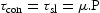
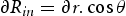
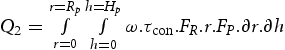
dA is the element of the cross-section area between matrix and tool surface. This element is expressed by its location and direction relative to tool rotation axis as shown in Figure 2. Circular and rectangular elements are used to calculate areas of the shoulder, probe base and probe tip (Figure 2 (a) and (c)).
Schematic drawing of surface orientations and infinitesimal segment. (a) Shoulder surface area, (b) Probe surface area and (c) Probe base and tip cross-section area.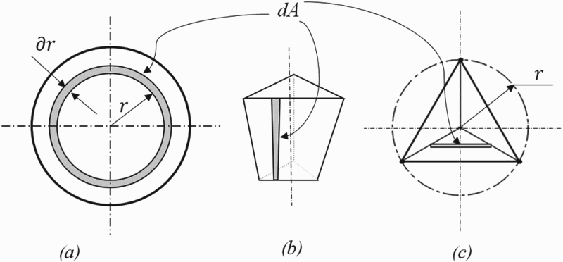
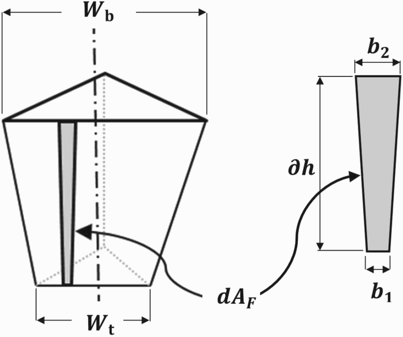
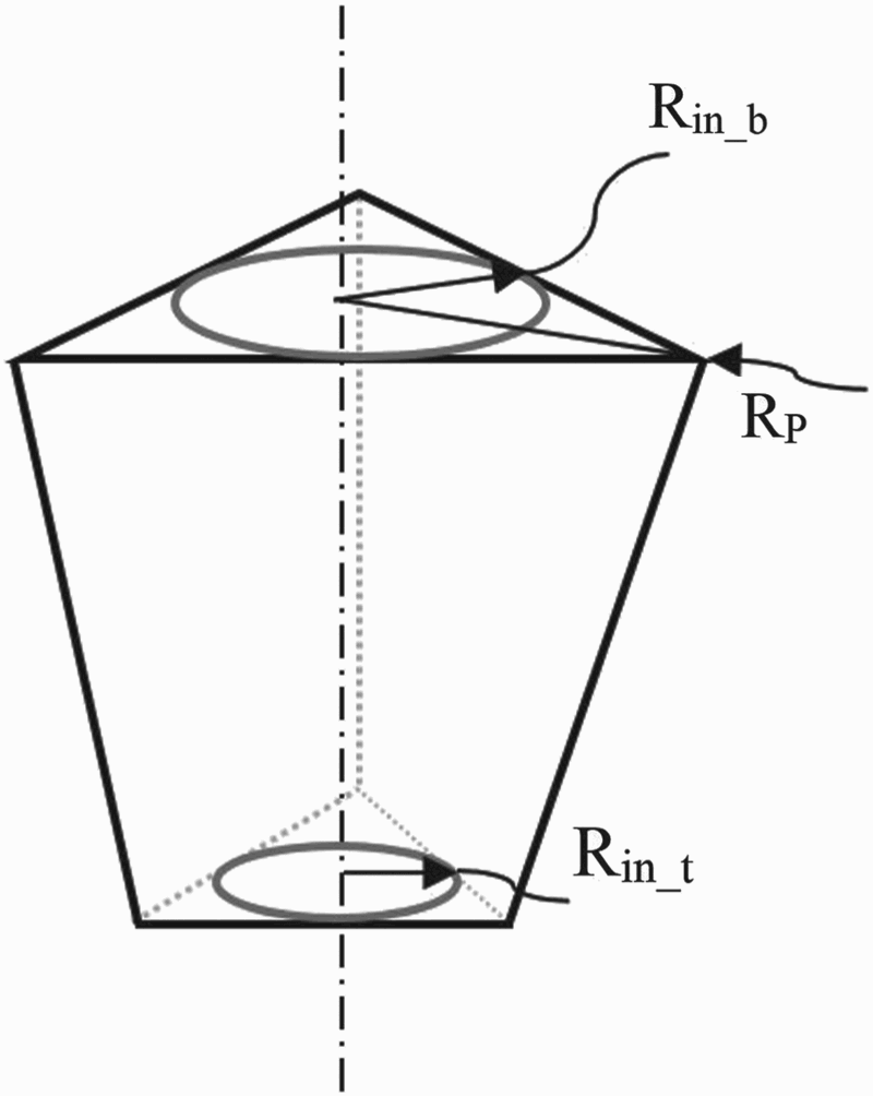
Probe base and tip cross-section element area dA are calculated by dividing this area into many triangles depending on the number of flats (N) as shown in Figure 3. dA can be calculated by:
Schematic drawing for probe base. (a) The triangular probe base cross-section. (b) Schematic drawing for position and dimensions of segment.
 is a height of element, it equals the change in radius of inscribed circle.
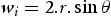
From Figure 3, wi is:
 is calculated by:


The values of radius factor (FR) and area factor (FA).
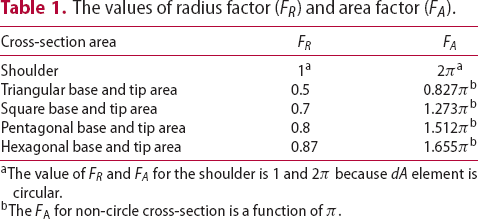
aThe value of FR and FA for the shoulder is 1 and 2π because dA element is circular.
bThe FA for non-circle cross-section is a function of π.
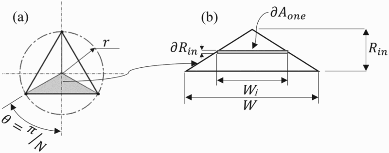
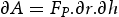
While the lateral probe surface area can be estimated by using isosceles trapezoidal elements (Figure 2 (b)). Polygonal probe surface area relies on a probe flats number, so probe surface area element (dA) calculates by:
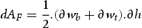
The element of area for one flat (dAF) can be expressed as (Figure 4):
Schematic drawing of isosceles trapezoidal element to probe surface.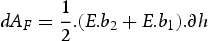
While E.b1 and E.b2 are wb and wt, respectively, so Equation (9) can be rewritten as:
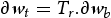
where Tr is the taper ratio, for present work, it is 0.6, so Equation (10) can be simplified to:
 can be expressed as:

dA is calculated by substitution of Equation (12) in Equation (8):

The values of radius factor (FR) and probe factor (FP).
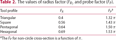
aThe FP for non-circle cross-section is a function of π.
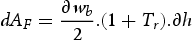
x is the shear force arm, i.e. it is the normal distance between the element area centre and probe central axis, its value for probe base, probe tip and probe surface can be calculated by:

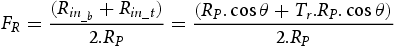
FR value for the probe base and probe tip is (Figure 5):
The radius of the inscribed circle at the probe base and probe tip cross-section.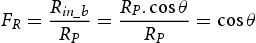
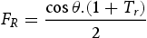
 for the probe surface is:
Heat generation in shoulder surface
The heat generated from the shoulder surface (
 ) is calculated by subtracting the heat generated by the probe base area
 from the heat generated at the shoulder
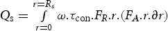
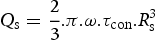
 . The QS can be calculated by substitution of Equation (7) and Equation (16) in Equation (1):
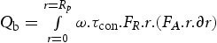
The heat generated by the probe base area
 can be expressed by substitution of Equation (7) and Equation (16) at Equation (1):
Equation (18) can be rewritten to become:
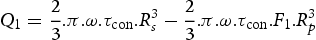
 is calculated from Qs to Qb, i.e. Equations (17) and (19).
Heat generation in probe surfaces
Heat generated from probe surface (
 ) is expressed by substitution Equation (15) and Equation (16) in Equation (1):
Equation (21) can be rewritten to become:
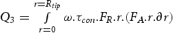
Heat generation in probe tip cross-section
Probe tip area heat generated
 can be expressed by substitution of Equation (7) and Equation (16) in Equation (1):
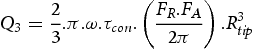
Equation (23) can be rewritten to become:
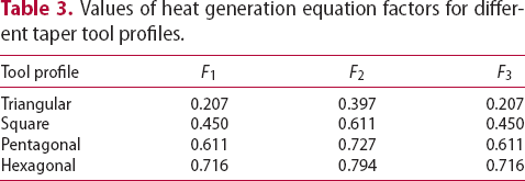
Values of heat generation equation factors for different taper tool profiles.
Validation
The thermal-pseudo-mechanical model (TPM) for the different taper probe profiles (TR, SQ, PEN and HEX) was developed using the heat transfer module in COMSOL 5.1. The model geometry was symmetric around the weld. The aluminium alloy AA 2014-T6 plate dimensions were 320 × 80 × 5 mm as shown in Figure 6.
Model geometry for FSW.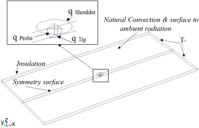
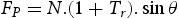
Tool rotational speed (N), weld speed (
 ) and axial force (Fn) were 1000 rev/min, 600 mm/min and 9 kN, respectively, for all tool profiles to study the effect of change in tool profile on the total heat generation. The temperature distribution was obtained from the steady-state conductive–convective energy equation (Equation (26) [18].

 is the density,
 the specific heat,
 the velocity vector,
 thermal conductivity, T the temperature and
 is the internal heat generation rate.
Two models (model 1 and model 2) were generated to predict the thermal profile for each tool with specific assumptions. These assumptions are listed in
Assumptions for models 1 and 2.
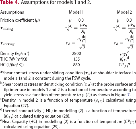
aShear contact stress under sliding condition (
 ) at shoulder interface in models 1and 2 is constant during the FSW cycle.
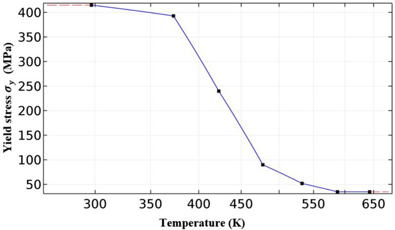
bShear contact stress under sticking condition (
Temperature-dependent 0.2% offset yield strength for AA 2014-T6 [25]. ) at the probe surface and tip interface in models 1 and 2 is a function of temperature according to yield stress as a function of temperature (σγ (T)) as shown in Figure 7.
cDensity in model 2 is a function of temperature (
 ) calculated using Equation (27).
dThermal conductivity (THC) in modelling (2) is a function of temperature (
 ) calculated using equation (28).
eHeat Capacity (HC) in modelling (2) is a function of temperature (
 ) calculated using equation (29).


where T is the temperature.
The data of physical properties (density, thermal conductivity, heat capacity) as a function of temperature in equations 27, 28 and 29 are calculated by JMatPro software.
Boundary conditions and initial condition
The heat flux boundary condition for the workpiece at the tool shoulder/workpiece interface is
 . Similarly, the heat flux boundary conditions at the probe lateral surface/workpiece interface and the probe tip/workpiece interface are
 and
and
 , respectively. The in-built material properties in COMSOL5.1 (density, thermal conductivity and heat capacity) for the AA 2014-T6 aluminium alloy were considered, and for AISI H13 tool steel, they are as follows: thermal conductivity –
 , density –
 and heat capacity at a constant pressure –
 [26]. The friction coefficient (
 ) was assumed constant at 0.3 [10].
Boundary conditions
The heat loss forms the upper plate's surface due convection and radiation; it can be expressed as:
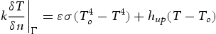
where k is the heat conductivity, ε is the emissivity, T is the temperature, n is a normal direction vector of boundary Γ,
 and
and
 are convection coefficients for lower and upper-base metal surfaces and
 is the initial temperature.
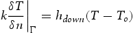
In the present project,
 and
and
 have different values because there is a contact between the lower surface and back-up plate. In the present study, it is considered as
 and
and
 , respectively. The emissivity (ε) was assumed to be 0.3 [10].
Initial condition
The initial condition for the calculation is:
 is the initial temperature.
Discussion
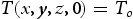
Figure 8(A–D) shows that peak temperature increases with number of flats TR (724 K), and SQ (743 K), PEN (758 K), and HEX tool profile (764 K). Kadian and Biswas [27] also showed that peak temperature increases with the increase in polygon probe sides. The present calculated results were about 81.5–83.6% of melting point. Biswas and Mandal [14] investigated the effect of tool profile on thermal profile. Their finding pointed that the ratio of peak temperature to melting point is more than 80%. Tikader et al. [28] reported that the ratio of peak temperature to melting point is increased by 10% with an increase in the probe diameter by 1 mm. Figure 9 compares peak temperature for different taper tool profiles under models 1 and 2 assumptions. It can be seen that the peak temperature increases by increasing the number of flats on the probe lateral surface in model 1 (TR (755 K), and SQ (775 K) PEN (791 K), and HEX (798 K)). In contrast, model 2 results showed the lowest peak temperatures compared with model 1.
Isotherms temperature distribution for different probe profiles: A-TR, B- SQ, C-PEN and D-HEX (model 2). Comparison between modelling results for the present work.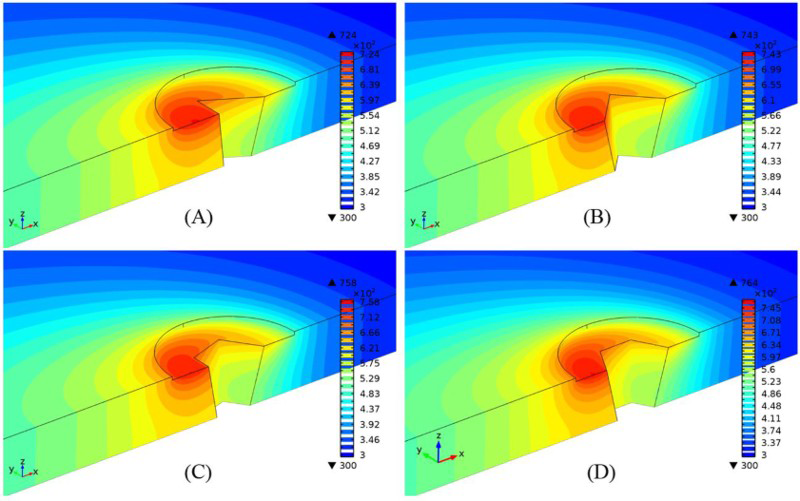
Model 2 results have a good agreement with the previous practical study [21] because it was considered the effect of change in physical material properties (density, thermal conductivity and heat capacity) with temperature on the thermal profile during welding cycle. HEX probe profile has the highest peak temperature because an increase in the number of flats in the probe surface leads to an increased deformation rate as a result of increasing stirring interaction and reducing rotating layer thickness [21] by a decrease in the effective stir dimension (the difference between inside and outside polygon radius for probe cross-section).
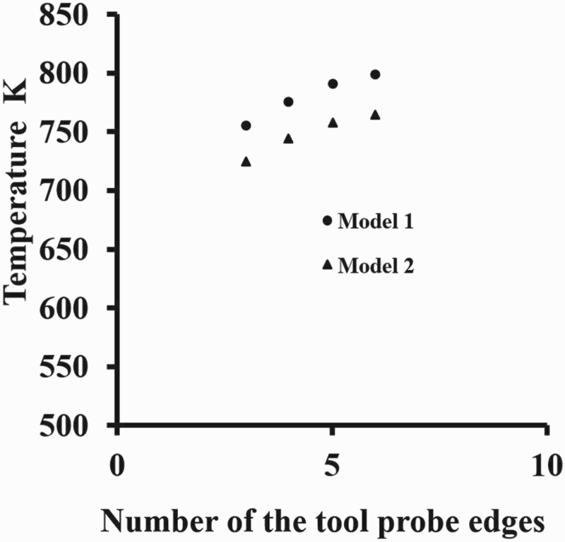
Modelling results for the present work are compared with experimental data measured by Ramanjaneyulu et al. [21] by calculating the temperature at specific point 3 mm from welding line (T_3 mm) at mid-thickness of plate because Ramanjaneyulu measured temperature at a point close to probe (approximately 3 mm).
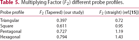
Good agreement is observed as shown in Figure 10. The variation between numerical model 1 results and practical results for Ramanjaneyulu et al. [21] is attributed to the following two reasons: The first reason is the material properties such as thermal conductivity, heat capacity and density for the workpiece are assumed constant and the second reason is the friction coefficient was assumed constant. The modelling results for the present work are also compared with numerical modelling results by Gadakh, Kumar et al. [15] who built their modelling according to practical results for Ramanjaneyulu et al. [21] as shown in Figure 10.
Multiplying Factor (F2) different probe profiles.
Conclusions
Equations
Equations for heat generation in FSW have been derived for different taper tool profiles such as TR, SQ, PEN and HEX. The major finding from the present work can be summarised as follows:
The amount of heat generation from shoulder surface decreases with increase of flats on the probe surface as a result of increase in the probe base area. The contribution of probe surface at total heat generation increases with increasing of flats on the probe surface as a result of increased deformation rate and contact area. The contribution of probe tip at total heat generation increases with increasing of flats on the probe surface as a result of increase in the contact area.
Validation
An analytical model for heat generation in FSW of aluminium alloy type AA 2014-T6 using different taper tool profiles such as TR, SQ, PEN and HEX is developed. The major findings from the present work can be summarised as follows:
The amount of heat generated as well as peak temperature is relatively high in non-circular taper probe profiles; they increase by increasing the number of edges for TR, SQ and PEN to reach maximum values in the HEX tool profile. The effective stir dimension is decreased by increasing the number of flats on surface probe profile. An increase in the number of effective stir dimension with an increase in the number of flats on the probe surface leads to an increase in the total heat generation.
By using the proposed analytical approach, we can predict the mechanical properties of a specific aluminium alloy by correlating the peak temperature for respective tool geometry under given FSW process conditions with the precipitate phase distribution and grain size.
Footnotes
Disclosure statement
No potential conflict of interest was reported by the authors.