Experimental evaluation of strain and strain rate during rapid cooling friction stir welding of pure copper

Abstract

The strain and strain rate during friction stir welding was evaluated by measuring the distortion of the marker material. A thin Cu-40Zn foil as marker was inserted into the butting surface of two pure copper workpieces and the tool ‘stop action’ was employed. The results show that the strain in the shoulder-affected zone increases in a two stair-step shape as the material flows from the front to the rear of the tool, corresponding to the first accelerated and then decelerated flow stages. However, the strain at the two stages has opposite directions. In other words, a strain reversal occurs. Accordingly, the strain rate in the shoulder-affected zone varies in a sinusoidal shape. In the probe-affected zone, there is no obvious strain reverse occurring due to the formation of banded structures. The average strain rate during the band formation is significantly higher than the maximum strain rate in the shoulder-affected zone.

Keywords

Friction stir welding strain strain rate pure copper material flow

Introduction

Friction stir welding (FSW) is generally accepted as a locally heated and large plastic deformation process, which usually leads to a significant microstructural refinement in the stir zone [1]. Rhodes et al. [2] suggested that nucleation and growth within a heavily deformed structure was the dominant mechanism for the formation of this fine-grain structure. Prangnell and Heason [3] revealed that the refined microstructure was actually the result of a slight grain coarsening during the cooling stage after the dynamic recrystallisation. Rapid cooling friction stir welding (RCFSW) is a modified FSW process, in which the cooling medium is directly exerted on the newly formed weld bead simultaneously with the FSW tool advancing. The rapid cooling can suppress the grain coarsening that occurred in the cooling stage of the FSW and therefore improve FSW joints’ mechanical properties. Xue et al. [4] achieved pure copper joints with nearly equal strength to the parent metal by RCFSW via flowing water. Xu et al. [5] improved the strength and ductility simultaneously in aluminium alloy joints by RCFSW with water cooling. Xu et al. [6, 7] obtained pure copper and Cu-30Zn joints with higher strength than the parent metal by RCFSW using liquid CO₂ cooling.

These studies show the great potential of RCFSW in the improvement of joints’ mechanical properties by suppressing the static annealing during the cooling stage of the FSW, and many studies [2, 3, 8] have revealed the recrystallisation mechanism during the FSW. However, a key issue, where is the limit of microstructural refinement at the plastic deformation stage of the FSW, is rarely addressed. This issue mainly involves the histories of the strain, strain rate and temperature during the FSW. The temperature history can be measured directly, though it may not be accurate due to the severe material flow. However, the strain and strain rate are difficult to obtain directly.

Researchers tend to obtain the strain and strain rate by numerical simulation methods. Nandan et al. [9] developed a three-dimensional viscoplastic flow and heat transfer numerical model, in which the strain rate was described together with the material flow ‘field’. It is difficult to correlate this kind of strain rate information with the actual microstructure evolution because the strain and strain rate histories which the material is subjected to are difficult to trace. Arora et al. [10] integrated the strain rate along a streamline to estimate the accumulated strain experienced by the materials based on a three-dimensional coupled viscoelastic flow and heat transfer model. This gives useful information on the strain and strain rate histories. Palanivel et al. [11] employed this method to calculate the shear-driven dissolution and fragmentation of thermally stable intermetallic particles during friction stir welding and processing. Unfortunately, the viscoplastic flow model has a congenital defect that it cannot simulate the non-continuous flow such as the banded structures formation in the probe-affected zone (PAZ) [12]. Therefore, there should be wide discrepancies between the evaluated strain and strain rate and the actual values in the PAZ. Tongne et al. [13] developed a finite element analysis model based on the Coupled Eulerian-Lagrangian formulation to predict the banded structures formed in the PAZ. They attributed the reason for the banded structures formation to the geometry of the pin (they used a trigonal shape pin). However, it cannot be explained reasonably why the banded structures still occur even though a smooth cylinder-shaped pin is used.

Recently, researchers have tried to develop some experimental methods to evaluate the strain and strain rate during the FSW. Liu et al. [14] employed the so-called marker insert method to evaluate the material flow velocity in the shoulder-affected zone (SAZ) and the nominal strain and strain rate in the PAZ. However, they did not evaluate the strain and strain rate in the SAZ. Morisada et al. [15] determined the strain rate during FSW by the three-dimensional visualisation of the material flow using tungsten sphere tracers and two sets of X-ray transmission real-time imaging systems. Kumar et al. [16] employed an experimental simulation method in which micro-spherical glass tracers in a transparent viscoplastic material together with the particle image velocimetry technique was used to approximate the strain rate during the FSW. Nevertheless, the strain was not obtained directly but reversely derived from the strain rate. In addition, as mentioned above, any methods based on the material flow velocity cannot be used to evaluate the strain and strain rate in the PAZ where non-continuous material flow occurs.

So far, there have not been unified methods to evaluate the strain and strain rate in the SAZ and PAZ simultaneously. Therefore, in this study, an experimental method based on the marker insert method was developed to approximately evaluate the strain and strain rate in the SAZ and PAZ during the RCFSW under the same standard, making them comparable. In this method, a thin marker material foil is inserted into the butting surface of the two workpieces. The strain and strain rate during the FSW can be directly evaluated based on the marker material distortion near the keyhole if a sudden ‘stop action’ of the FSW tool is used.

Experimental

Figure 1 shows a schematic of the experiment. Three millimetre-thick commercial pure copper C1100P in the 1/4H condition was used as the parent material. A thin foil of Cu-40Zn brass (0.5 mm nominal thickness) was pre-set into the butting surface of the two workpieces as the marker material. The pure copper and Cu-40Zn system shows a good solid solution and no brittle intermetallic compound formation over the whole processing temperature range. In addition, the Cu-40Zn brass has a duplex-phase structure, which leads to very low flow stress at high temperatures. Xiao et al. [17] reported that the flow stress of Cu-40Zn brass is only ∼40 MPa at 650°C (close to the welding peak temperature [18]) and strain rate of 1 s⁻¹. However, for the same deformation condition, the flow stress of pure copper is ∼100 MPa according to the studies of Huang et al. [19] and Zhao et al. [20]. This indicated that the Cu-40Zn brass can deform compatibly together with the pure copper at the FSW conditions. The tool sudden ‘stop action’ was applied using the emergency stop, which indicates that the FSW machine lost power suddenly and the tool was pulled out immediately. In the RCFSW, liquid CO₂ was jetted onto the fresh weld surface rapidly through two tandem pipes and was moved with the FSW tool simultaneously [21].

Figure 1

Schematic of the experiment.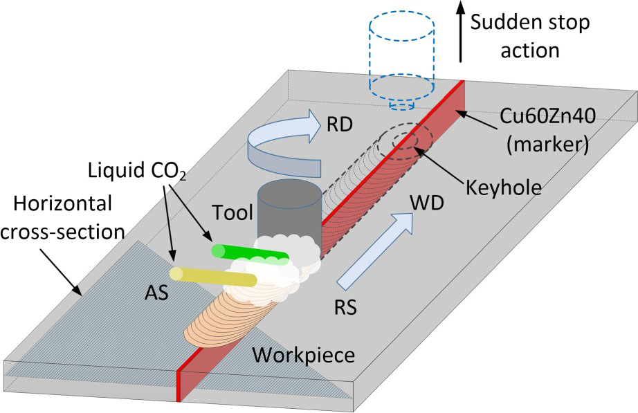

As for the welding parameters, a tungsten-carbide-based alloy tool containing a concave shoulder of 12 mm diameter and a smooth cylindrical probe of 4 mm diameter and 2.8 mm length was used. The tilt angle of the tool was 3°. The FSW machine was operated in a displacement control mode. The welding and rotating speeds were 150 mm min⁻¹ and 800 rpm, respectively.

After welding, the specimen containing the keyhole was collected via wire-cutting. In order to evaluate the strain and strain rate in the SAZ and PAZ, respectively, the specimen was ground 0.5 mm from the top and bottom using sandpapers in flowing water, defined as the 0.5-mm-plane (upper part) and 2.5-mm-plane (lower part, 0.5 mm from the bottom), respectively. Their metallographic specimens were prepared via mechanical polishing and subsequent etching with a solution of FeCl₃ (5 g) + HCl (25 mL) + H₂O (75 mL). The metallographic photographs for each plane were obtained using an optical microscope and were spliced to obtain a panoramic view.

Results and discussion

Material flow patterns

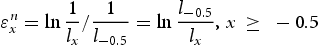
Figure 2 shows the macro-metallographic photos of the selected horizontal planes of the keyhole. A uniaxial coordinate system was established to describe the deformation characteristics at various locations. The keyhole center was set as the origin and the material feed direction (the opposite of the welding direction, WD) was set as the positive direction. The dimensions are in millimeters. In the upper weld part (Figure 2(a), 0.5-mm-plane), the long strip-shaped marker material was deformed into a continuous, curving and non-uniform-thickness strip. However, in the lower part (Figure 2(b), 2.5-mm-plane: 0.5 mm from the bottom), the distribution of the marker material is discontinuous. Behind the keyhole, it presents a periodic banded structure. Generally, the zone where a continuous material flow pattern is observed is defined as the SAZ, while the zone where a banded structure is formed is called the PAZ as proposed by Liu et al. [14] and Liu and Wu [12, 22]. Therefore, the material flow on the 0.5-mm-plane can be used as an example representing the material flow in the SAZ, while the material flow on the 2.5-mm-plane can be used to represent the material flow in the PAZ. According to the deformation of the marker material in Figure 2, the material flow both on the 0.5-mm-plane and the 2.5-mm-plane can be roughly divided into five stages.

Figure 2

Macro-metallographic photos of the 0.5-mm-plane (a) and 2.5-mm-plane (b). Note: WD, welding direction; RD, rotating direction.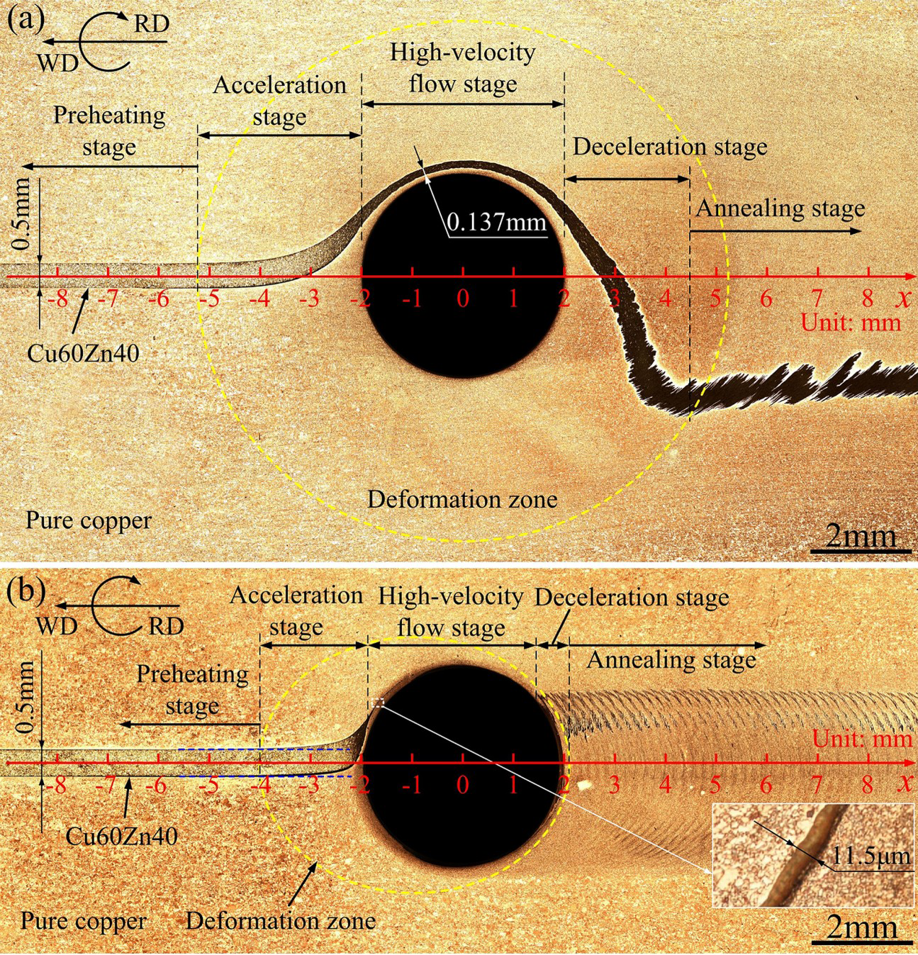

On the 0.5-mm-plane, first, the material in the region x < −5.2 has not yet started to deform, while the material may be subjected to heating due to the heat generation in the stir zone. Therefore, this stage is defined as the preheating stage in this study. Although no strain occurs at the preheating stage, it is believed that this stage will play an important role in the FSW of work hardened materials. Second, in the range of −5.2 < x < −2, the position of the marker material has deviated from the original butting line and its thickness decreases gradually. This means that the material flow velocity and plastic strain increase gradually, and thus this stage is defined as the acceleration flow stage. Thirdly, from x = −2 to x = 2, near the keyhole, the thickness of the marker material remains very thin and only slightly changes. The smallest thickness is 0.137 mm. This stage is defined as the high-velocity flow stage. Fourthly, from x = 2 to x = 4, the thickness of the marker material recovers to the initial thickness gradually, which means that the material flow velocity decreases gradually and the plastic deformation is finished at x = 4. This stage is defined as the deceleration flow stage. Finally, out of the stir zone (x > 4), the material will undergo afterheat and annealing may occur. Therefore, this stage is defined as the annealing stage. In the RCFSW, the cooling medium mainly influences this stage and suppresses the static annealing.

On the 2.5-mm-plane, due to the absence of the shoulder's effect, the deformation zone around the keyhole is much smaller than that on the 0.5-mm-plane, as shown by the ellipse region enclosed by the yellow short-dashed line in Figure 2(a,b). The beginning point of the deformation zone is determined by the marker material beginning to deviate from the original position, as depicted by the blue short-dashed line in Figure 2(b). The ending point is determined by the periodicity of the marker material distribution reaching a stable state. It can be seen that the deformation zone in front of the keyhole is much larger than that behind the keyhole. This should be attributed to the pressure on the front side caused by the relative motion between the workpieces and the tool. Similar to the 0.5-mm-plane, the material flow on the 2.5-mm-plane can also be divided into five stages: the preheating stage (x < −4), the acceleration flow stage (−4 < x < −2), the high-velocity flow stage (−2 < x < 1.4), the deceleration flow stage (1.4 < x < 2) and the annealing stage (x > 2), as shown in Figure 2(b). However, the plastic strain of the material at the high-velocity flow stage on the 2.5-mm-plane should be much higher than that on the 0.5-mm-plane. Within the visible range, the thickness of the marker material is only 11.5 μm (as marked in Figure 2(b)), which is 8.4% of the corresponding value on the 0.5-mm-plane. This should be attributed to the less distance from the marker material to the probe surface and the smaller deformation zone on the 2.5-mm-plane.

Owing to the non-continuous material flow, the deceleration process on the 2.5-mm-plane is significantly different from that on the 0.5-mm-plane. On the 0.5-mm-plane, it appears that the material gradually accumulates along the material flow path due to the decrease in driving force at the deceleration flow stage. This process looks like an inverse process in contrast with that occurring at the acceleration flow stage, where the marker material was stretched and became thinner and thinner. Therefore, if the strain occurring at the acceleration flow stage is defined as positive, the strain that occurred at the deceleration flow stage must be negative. However, on the 2.5-mm-plane, the material appears to be released suddenly by the rotating tool, because the marker material does not converge into one strip, but keeps its stretched shape, and deposits on the weld bead, as shown by the banded structure in Figure 2(b).

Strain and strain rate in SAZ

In this section, the distortion of the marker material on the 0.5-mm-plane is used to evaluate the strain and strain rate in the SAZ.

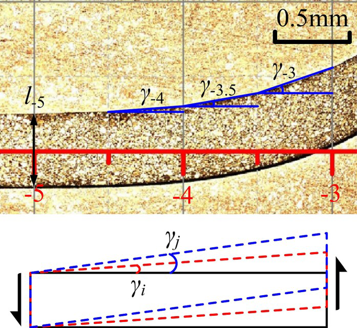
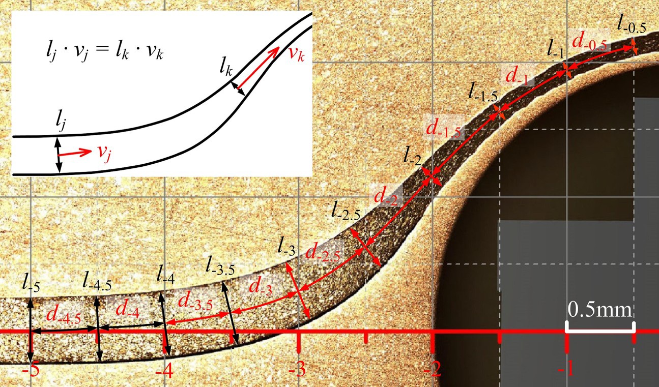
On the 0.5-mm-plane, from a panoramic view of the distribution of the marker material, the deformation model during FSW can be approximated to three classes. First, at the initial deformation stage (x ≤−3), the thickness of the marker material strip does not evidently change, but the marker material strip deviates from its initial position with the increase in angle γ, as shown in Figure 3. This kind of deformation can be approximately regarded as simple shear deformation. The nominal strain ϵ can be calculated using the following equation: (1) The equivalent accumulative true strain can then be approximately given by: (2) where , and are the nominal strain, deviated angle and accumulative true strain at the location x (x ≤−3), respectively.

Figure 3

Approximate deformation model at x ≤−3 on the 0.5-mm-plane.

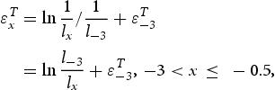
In the interval −3 < x ≤−0.5, the thickness of the marker material strip gradually decreases. Although this deformation results from a simple shear deformation, the driving force for the marker material flow should simultaneously come from both the shoulder and the probe. The shear force is not exerted on the marker material from only one side, but from multiple sides at the same time. In addition, due to the fact that the marker material strip is very thin, the velocity gradient of the two sides of the marker material strip must be very low (actually, the velocity of the inner side may larger than that of the outer side due to the tool advancing). Therefore, the deformation in the interval −3< x ≤−0.5 can be approximately equivalent to a tensile strain in the material flow direction if only the change in geometry shape is considered, as shown in Figure 4. For the sake of simplification, it is assumed as plane strain tension. Thus, the accumulative true strain can be roughly evaluated by the changes in the marker material thickness l: (3) where and are the thickness of the marker material strip and the accumulative true strain,respectively, at the location x = −3, and and are the thickness of the marker material strip and the accumulative true strain, respectively, at the location x (−3< x ≤−0.5), as shown in Figure 4.

Figure 4

Approximate deformation model at −3 < x≤−0.5 on the 0.5-mm-plane.

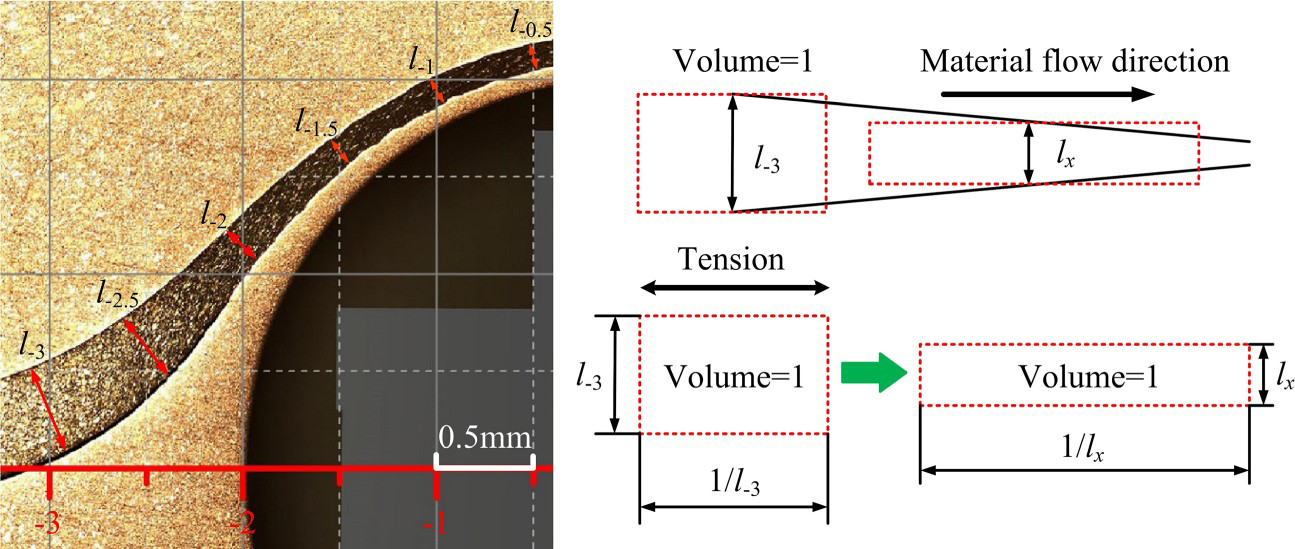
For x ≥ −0.5, the thickness of the marker material strip begins to increase. Owing to the decrease in the driving force of the tool, the marker material is accumulated gradually in the material flow direction, resulting in the increase in the marker material strip thickness. In addition, the driving force from the probe side may rapidly decrease due to the tool advancing, while the driving force from the shoulder may not obviously decrease because the shoulder still covers the deforming material. This may cause that the material flow velocity of the inner side is smaller than that of the outer side of the marker material stripe. Therefore, relative to the shear strain in the interval −3< x ≤−0.5, the shear strain in this stage should have the opposite direction (defined as negative in this study). Therefore, the deformation from x ≥ −0.5 is approximately regarded as a compressive strain in the material flow direction, as shown in Figure 5. Similarly, for the sake of simplification, it is assumed as plane strain compression. The negative (self-defined) shear true strain can be approximately evaluated using the following equation which is similar to Equation (3): (4) Thus, the accumulative true strain can be given by the following equation: (5)

Figure 5

Approximate deformation model at x ≥ −0.5 on the 0.5-mm-plane.

where and are the thickness of the marker material strip and the accumulative true strain,respectively, at the location x = −0.5; and are the thickness of the marker material strip and the negative (self-defined) shear true strain, respectively, at the location x (x ≥ −0.5), as shown in Figure 5. is a correction factor that represents the effect of the strain path reversal [23].

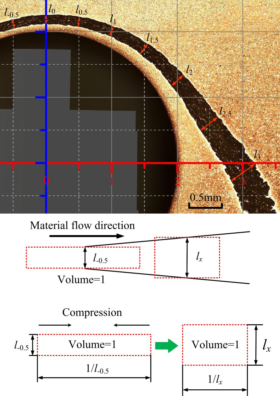
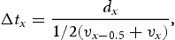
In order to calculate the strain rate, the deformation time between two measured points is necessary. The material flow in the passageway formed by the marker material on the horizontal plane of the keyhole can be approximated to a one-dimensional incompressible fluid flow [14] (assuming that the workpieces move relative to the FSW tool, the same as below). Thus, it satisfies the one-dimensional continuity equation, i.e. the flux of the fluid flowing at any two cross-sections is equal at any instance, as shown in Figure 6. The material flow velocity at a given location x is formulated as: (6) where and are the initial thickness of the marker material strip and the initial material flow velocity, respectively, and and are the thickness and the velocity at location x, respectively.

Figure 6

Schematic of the measurement and calculation of the material flow velocity and deformation time on the 0.5-mm-plane.

Using the average value of the velocities at two adjacent measured points as the average material flow velocity of the corresponding interval, the deformation time between two adjacent measured points is given by (7) where is the time interval between the locations [x−0.5] and x, and are the corresponding material flow velocities, and is the curvilinear distance along the marker material strip between the locations [x−0.5] and x, as shown in Figure 6.

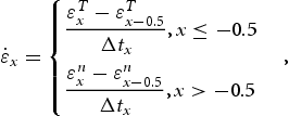
Thus, the true strain rate can be evaluated by the following equation: (8) where represents the average strain rate of the interval between the locations [x−0.5] and x.

The obtained strain, material flow velocity and strain rate on the 0.5-mm-plane are shown in Figure 7. Here is assumed to be 1, which indicates that the geometric effect of the strain is the main consideration. The curve of the accumulative true strain presents a two stair-step shape. It contains two stages, i.e. the positive shear strain stage and the negative (self-defined) shear strain stage, corresponding to an initial decrease and subsequent increase in the thickness of the marker material strip. The increase in the accumulative strain at the two stages is similar, and the total true strain reaches ∼2.7, which is comparable with the simulated results by Arora et al. [10]. Nevertheless, the strain reverse is noticeable. The material flow velocity with respect to the locations in the x direction shows a unimodal distribution. Similar to the observed results in Figure 2, the calculated material flow velocity begins to increase significantly at the location x = −3, thereafter rapidly reaches the peak value of 8.97 mm s⁻¹ at the location x = −0.5, and finally decreases to 2.5 mm s⁻¹ at the location x = 4, which is the same value as the initial velocity. The calculated strain rate is very interesting and shows an approximately sinusoidal distribution. At the stretching stage, a peak is located at x = −1.5 with a value of 3.29 s⁻¹, which corresponds to the sharp acceleration of the material flow as the material approaches the probe. At the compression stage, a peak value of −2.20 s⁻¹ is observed at the location x = 2, which corresponds to the sharp decrease in the material flow velocity and is slightly weaker than the first peak. The measured strain rates are of the same order of magnitude as the simulated results by Arora et al. [10].

Figure 7

Distributions of strain, material flow velocity and strain rate in x direction on the 0.5-mm-plane.

Strain and strain rate in PAZ

In this section, the distortion of the marker material on the 2.5-mm-plane is used to evaluate the strain and strain rate in the PAZ.

On the 2.5-mm-plane, due to the discontinuous material flow, the above method is no longer appropriate for calculating the strain and strain rate. Liu et al. [14] proposed a method to evaluate the strain and strain rate for this kind of banded structure. However, the effect of the non-continuous material flow was neglected in calculating the strain and strain rate in front of the keyhole. In this study, a new approximate method is proposed to calculate the true strain and strain rate for the banded structure on the 2.5-mm-plane. The model is shown in Figure 8.

Figure 8

Schematic of the measurement and calculation of the strain and strain rate on the 2.5-mm-plane.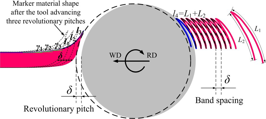

When the marker material strip thickness has no obvious change, the true strain can be evaluated using Equation (2), i.e. . The true strain rate can be calculated using Equation (8). If the thickness of the marker material strip decreases apparently, Equation (2) is no longer applicable. In this case, it can be imagined that if the tool advances one revolutionary pitch, , the marker material shape in front of the probe would change as the dashed line shown in Figure 8. At the same time, a new band would be formed behind the probe. The stretching of the marker material in front of the probe during one revolution, , can be evaluated approximately by the spacing between two adjacent imagined marker material shape profiles (the dashed line) along the streamline, as recorded by l₁, l₂ and l₃ in Figure 8. In addition, the stretching of the marker material during one revolution, , behind the probe can be measured according to the length of one band, as recorded by l₄ in Figure 8. Thus, the true strain can be approximately evaluated as follows: (9) where is the revolution pitch and is the stretching of the marker material during one revolution. The true strain rate, , over the time required to complete a revolution, Δt, can be calculated as follows: (10)

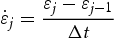
The calculated results are shown in Figure 9. The accumulative true strain in front of the probe is 1.03 and the strain rate is as high as 9.47 s⁻¹. After the band formation, the accumulative true strain reaches ∼2.59, and the average true strain rate during the band formation is as high as 20.8 s⁻¹. When transformed into the nominal strain and strain rate, they are equivalent to 12.5 and 140 s⁻¹, respectively, which have the same order of magnitude as the results (34 and 103 s⁻¹, respectively) obtained during the FSW of 2024 Al-alloy by [14]. In contrast to the strain and strain rate in the SAZ, there is no obvious strain reversal occurring in the PAZ. In addition, the average strain rate during the band formation is significantly higher than the strain rate in the SAZ. Foreseeably, these complicated strain and strain rate distributions must have significant effect on the grain refinement during the FSW. Further investigation will be done to clarify these problems in the next study.

Figure 9

Distributions of strain, material flow velocity and strain rate in x direction on the 0.5-mm-plane.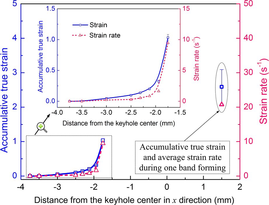

Notably, the measured maximum strain and strain rate do not represent the maximum values occurring during the entire FSW because the strain and strain rate distributions are inhomogeneous and the maximum values may not occur in the marker material flow line.

Conclusions

A series of measurements and calculations based on the distortion of the marker material during FSW have been developed to evaluate the strain and strain rate distribution during the RCFSW of pure copper. The following conclusions can be drawn:

Two approximate methods have been developed to evaluate the strain and strain rate for the continuous material flow pattern in the SAZ and the non-continuous material flow pattern in the PAZ.

An obvious strain reverse occurs in the SAZ, while it is negligible in the PAZ.

The accumulative strain in the SAZ increases in a two stair-step shape as the material flows from the front side to the rear side of the probe. The maximum strain in the butting line reaches ∼2.7.

The strain rate in the SAZ varies in a sinusoidal shape as the material flows from the front side to the rear side of the probe, with a positive peak value of 3.29 s⁻¹ at the acceleration flow stage and a negative peak value of −2.20 s⁻¹ at the deceleration flow stage.

In the PAZ, the accumulative strain reaches ∼2.59 after the band formation. The average strain rate during the band formation is 20.8 s⁻¹, which is significantly higher than the maximum strain rate in the SAZ.

Footnotes

Disclosure statement

No potential conflict of interest was reported by the authors.

References

Mishra

, Ma

ZY.

Friction stir welding and processing. Mater Sci Eng R. 2005; 50:1–78. doi: 10.1016/j.mser.2005.07.001

Rhodes

, Mahoney

, Bingel

, Fine-grain evolution in friction-stir processed 7050 aluminum. Scr Mater. 2003; 48:1451–1455. doi: 10.1016/S1359-6462(03)00082-4

Prangnell

, Heason

CP.

Grain structure formation during friction stir welding observed by the ‘stop action technique’. Acta Mater. 2005; 53:3179–3192. doi: 10.1016/j.actamat.2005.03.044

Xue

, Xiao

, Zhang

, Achieving friction stir welded pure copper joints with nearly equal strength to the parent metal via additional rapid cooling. Scr Mater. 2011; 64:1051–1054. doi: 10.1016/j.scriptamat.2011.02.019

, Liu

, Chen

, Improvements of strength and ductility in aluminum alloy joints via rapid cooling during friction stir welding. Mater Sci Eng A. 2012; 548:89–98. doi: 10.1016/j.msea.2012.03.094

, Ueji

, Morisada

, Modification of mechanical properties of friction stir welded Cu joint by additional liquid CO₂ cooling. Mater Des. 2014; 56:20–25. doi: 10.1016/j.matdes.2013.10.076

, Ueji

, Fujii

Enhanced mechanical properties of 70/30 brass joint by rapid cooling friction stir welding. Mater Sci Eng A. 2014; 610:132–138. doi: 10.1016/j.msea.2014.05.037

McNelley

, Swaminathan

, Su

JQ.

Recrystallization mechanisms during friction stir welding/processing of aluminum alloys. Scr. Mater. 2008; 58:349–354. doi: 10.1016/j.scriptamat.2007.09.064

Nandan

, Roy

, Lienert

, Three-dimensional heat and material flow during friction stir welding of mild steel. Acta Mater. 2007; 55:883–895. doi: 10.1016/j.actamat.2006.09.009

10.

Arora

, Zhang

, De

, Strains and strain rates during friction stir welding. Scr Mater. 2009; 61:863–866. doi: 10.1016/j.scriptamat.2009.07.015

11.

Palanivel

, Arora

, Doherty

, A framework for shear driven dissolution of thermally stable particles during friction stir welding and processing. Mater. Sci. Eng. A. 2016; 678:308–314. doi: 10.1016/j.msea.2016.10.015

12.

Liu

, Wu

CS.

Material flow in ultrasonic vibration enhanced friction stir welding. J Mater Process Technol. 2015; 225:32–44. doi: 10.1016/j.jmatprotec.2015.05.020

13.

Tongne

, Desrayaud

, Jahazi

, On material flow in friction stir welded Al alloys. J Mater Process Technol. 2017; 239:284–296. doi: 10.1016/j.jmatprotec.2016.08.030

14.

Liu

, Wu

, Padhy

GK.

Characterization of plastic deformation and material flow in ultrasonic vibration enhanced friction stir welding. Scr Mater. 2015; 102:95–98. doi: 10.1016/j.scriptamat.2015.02.022

15.

Morisada

, Imaizumi

, Fujii

Determination of strain rate in friction stir welding by three-dimensional visualization of material flow using X-ray radiography. Scr Mater. 2015; 106:57–60. doi: 10.1016/j.scriptamat.2015.05.006

16.

Kumar

, Pancholi

, Bharti

RP.

Material flow visualization and determination of strain rate during friction stir welding. J Mater Process Technol. 2018; 255:470–476. doi: 10.1016/j.jmatprotec.2017.12.034

17.

Xiao

, Guo

XY.

Constitutive modeling of hot deformation behavior of H62 brass. Mater Sci Eng A. 2011; 528:6510–6518. doi: 10.1016/j.msea.2011.04.090

18.

Mironov

, Inagaki

, Sato

, Microstructural evolution of pure copper during friction-stir welding. Phil Mag. 2015; 95:367–381. doi: 10.1080/14786435.2015.1006293

19.

Huang

, Shu

, Hu

, Effect of strain rate and deformation temperature on strain hardening and softening behavior of pure copper. Trans Nonferrous Met Soc China. 2016; 26:1044–1054. doi: 10.1016/S1003-6326(16)64201-2

20.

Zhao

, Liu

, Tian

, High temperature deformation behavior of pure copper. Heat Treat Met. 2011; 36:17–20. Chinese.

21.

Fujii

, Chung

, Sun

YF.

Friction stir welding of AISI 1080 steel using liquid CO₂ for enhanced toughness and ductility. Sci Technol Weld Join. 2013; 18:500–506. doi: 10.1179/1362171813Y.0000000128

22.

Liu

, Wu

CS.

Elimination of tunnel defect in ultrasonic vibration enhanced friction stir welding. Mater Des. 2016; 90:350–358. doi: 10.1016/j.matdes.2015.10.131

23.

Humphreys

, Hatherly

Recrystallization and related annealing phenomena. Oxford: Elsevier; 2004; pp. 222–224.