Stress measurement and correction with contour method for additively manufactured round-rod specimen

Abstract

The contour method (CM) was applied to obtain residual stress field in the round-rod titanium alloy specimen fabricated by laser power bed fusion additive manufacturing. In order to improve the accuracy of CM, two methods were investigated. One employed a steel block glued to the specimen to shift the surface stress uncertainties. The other is to reconstruct the stress based on the eigenstrain inverse analysis method. Results show that both methods can improve the measurement accuracy on the surface layer stress to a certain extent. Attaching steel block would affect the cutting process and cause new test errors. The stress reconstruction method requires surface stress results and eigenstrain basis function with an order of at least 10.

Keywords

Round-rod specimen residual stress contour method eigenstrain stress correction

Introduction

Additive manufacturing (AM) is a process in which material is deposited layer by layer to build up a three-dimensional object [1]. This facilitates or enables the rapid production of prototype geometries and complex morphologies, making AM an attractive process for the metal production of low-volume parts and novel complex shapes [2]. There are also some intrinsic characteristics of the as-deposited metal parts, such as large columnar grains, high residual stress, distortions, micro-voids, or even cracks [3, 4], which are caused by a strong temperature gradient, high cooling rate, and high solidification front velocity during the process of very localised melting and solidification.

The residual stress, especially high tensile residual stress, has detrimental effects on the overall deformation and dimensions, fatigue strength, and fracture toughness of parts [5]. Knowing the distribution of the residual stress is the key factor to mitigate the residual stress, and then improve the service performance of the metallic structures. It is also very important to obtain the internal stress distribution in additively manufactured components for optimising the additive manufacturing process, the structural design, and the heat treatment strategy of stress mitigation. The contour method (CM) [6] is a completely destructive stress measurement method, which can obtain the whole two-dimensional map of stress distribution inside a component. In this method, the specimen is cut into two halves on the plane of interest, so that the residual stresses in the specimen are relaxed and cause the deformation of the cut planes. Then the displacements on the cut planes are measured and adopted to construct the stress distribution based on the finite element analysis.

The CM has been applied to get the full map stress distribution in AM specimens [7 -10]. However, due to the limitations of cutting and surface deformation measurement [6], there are large uncertainties existed in the surface layer stress obtained by the CM [11], especially for the round-rod specimen. In the present study, the residuals stress in the round-rod specimens prepared by laser power-bed fusion (L-PBF) additive manufacturing (AM) were measured by CM. The surface stress was measured by the X-ray diffraction method. The axial stress distribution in the round-rod titanium alloy specimen fabricated by L-PBF is obtained. Two methods to improve the stress measurement accuracy of the CM in the surface layer were investigated. One employs a steel block glued to the specimen with the electrically conductive adhesive, then the surface errors during cutting and deformation measurement can be transferred to the surface of the block. The other is the stress reconstruction based on the eigenstrain method.

Specimen preparation

The round-rod specimen was prepared with the L-PBF method using the Ti6Al4V powder. The average diameter of the power is about 38 µm. The specimen has a diameter of 16 mm and a length of 70 mm, as shown in Figure 1(a). Two specimens with the same dimensions were prepared using the L-PBF method and the same parameters. One specimen is used to measure the axial stress with the common contour method without any strategy to reduce the displacement error. The other was measured under the condition with two steel blocks attached to reduce the displacement error (the method is introduced in the following section). Two specimens are prepared by a commercial EOS-M280 manufacturing system. The manufacturing parameters are the same as those introduced in Ref. [12]. The laser power ranges from 260 to 300 W, the scanning speed lies in the range from 1000 mm s⁻¹ to 1400 mm s⁻¹. A ‘back and forth’ hatch pattern was employed with the scanning direction of each newly deposited layer rotated by 67° with respect to the previous one. The layer thickness of 30 µm and hatch spacing of 0.14 mm was adopted.

Figure 1

(a) The Ti6Al4V round-rod specimen; (b) contour measurement after cut.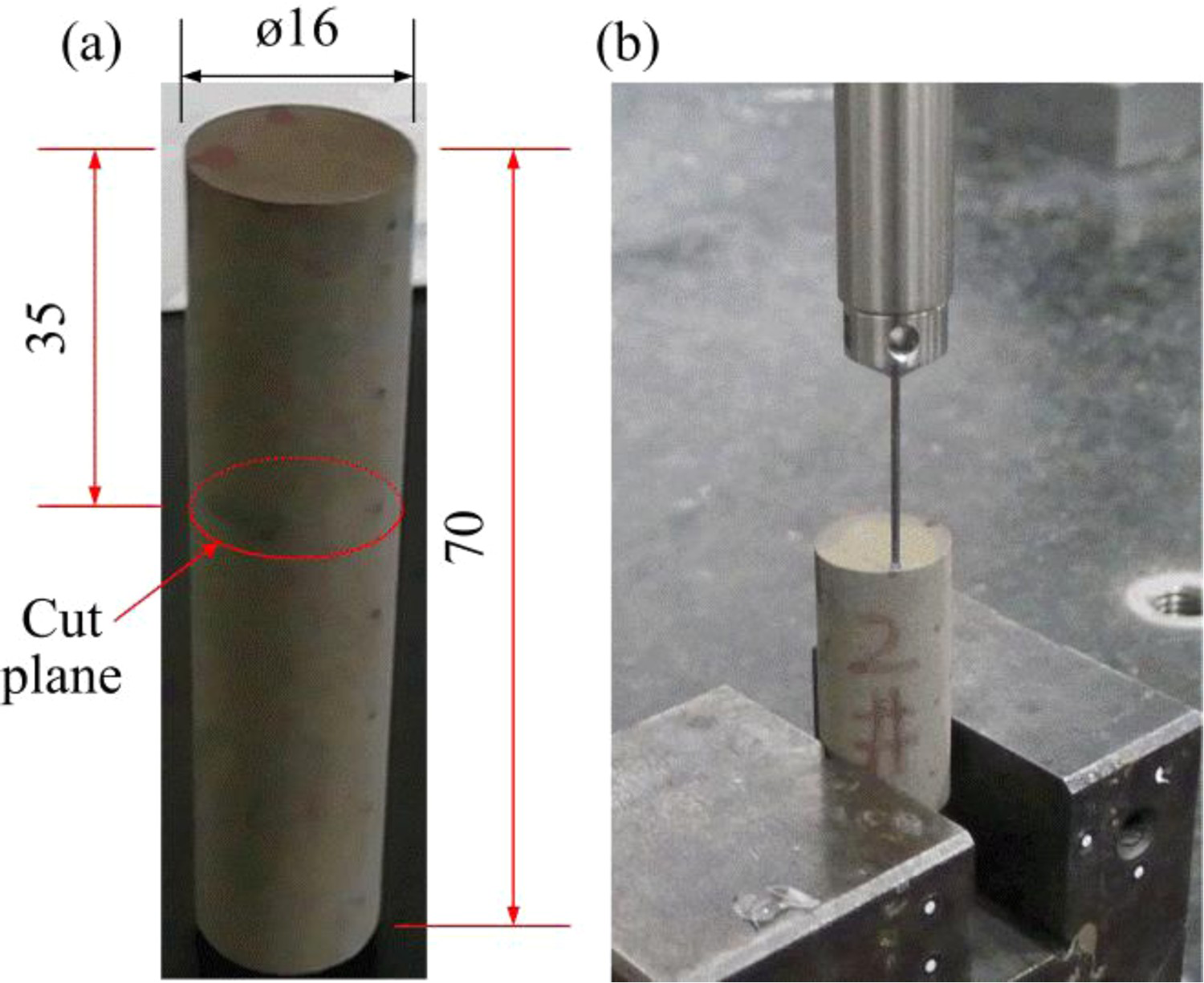

Residual stress measurement

X-ray diffraction method

The X-ray diffraction (XRD) method was adopted to measure the surface stress. Several points on the surface near the location of the mid-length were measured. The device proto LXRD was adopted to perform the measurement using the constant ψ₀ method to analyse the lattice planes {213} diffraction peaks with a Cu-kα radiation source.

Contour method

Application of the contour method primarily involves four steps: specimen cutting, contour measurement, data processing, and finite element analysis. The CM procedure is introduced based on the round-rod specimen in this study.

First, the part is securely clamped in a special fixture and cut into two halves at the location of the mid-length using a wire electric discharge machine (EDM). The goal of the clamping is to minimise movement of the part during cutting. The use of wire EDM is preferred because the cutting action is localised to the cut tip and the quality of the cut is high. A Seibu M50 EDM was adopted to perform the cut in the present study with a cutting speed of about 0.3 mm min⁻¹.

After the cut, the cut surface topography of each half is measured using a Zeiss coordinate measuring machine (CMM). The measurement space is 0.25 mm in both radial and hoop directions. The photo of the displacement measurement is shown in Figure 1(b). The displacements on the cut planes are then processed by deleting the singular points, averaging each pair of measured points, and smoothing with a bivariate spline smoothing algorithm. Finally, a finite element (FE) model is built according to the dimensions of the after-cut specimen and the smoothed surface contours are introduced to the FE model as displacement boundary conditions, and the original stresses on the cut plane are back-calculated by an elastic FE analysis. In the present study, the Young's modulus of the material was assumed to be 105 GPa with 0.33 for the Poisson's ratio. Three additional displacement constraints were applied to the model to avoid rigid body motion.

Displacement error in CM and improvement methods

Displacement error in CM

During EDM cutting, the melting metal could recast on the surface, resulting in a recast layer and rough surface [13]. Therefore, the EDM cut itself would lead to a rougher cutting quality in the surface layer than in the interior. In addition, the spherical tip of the CMM probe would go slightly past the edge of the part when measuring the displacement [6], which also results in stress error at the specimen edge. For the round-rod specimen, the cut thickness during EDM cut is constantly changing, making it difficult to maintain constant cutting, so that additional displacement error would occur, especially on the surface layer. The uncertainty associated with the noise in the displacement data is collectively known as the displacement error in CM [14].

Attaching steel block method

Two steel blocks are glued to the round-rod specimen using the conductive adhesive, thus the round-rod specimen becomes a rectangle block and the cutting thickness keeps constant during EDM cutting. The displacement of the steel block was discarded when reconstructing the stress distribution for the second step of the CM. The steel block attached to the round-rod specimen is also called the sacrificial block, as described in Ref. [15] The schematic diagram of the specimen and the after-cut section of the specimen with the sacrificial block is shown in Figure 2.

Figure 2

(a) Schematic diagram of attaching steel blocks; (b) cutting specimen after attaching steel blocks;(c) after-cut section.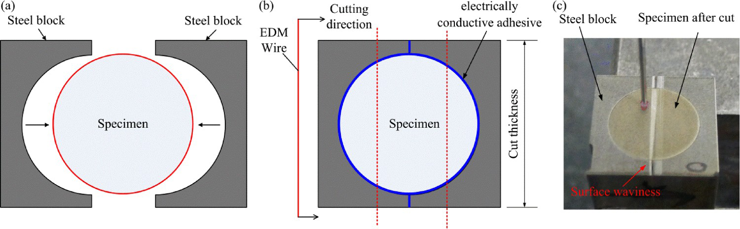

Eigenstrain method of stress reconstruction

The eigenstrain method was adopted to reconstruct the stress distribution in Specimen 1 using part of the measured results of the CM and the XRD surface stress results to improve the measurement accuracy at the edge of the round-rod specimen. The term eigenstrain designates any kind of permanent incompatible strain in a body that arises due to some inelastic process such as plastic deformation, crystallographic transformation, thermal expansion mismatch between different parts of an assembly, etc. [16]. Eigenstrain is an intrinsic parameter that can be thought of as the origin (or the source) of residual stress, as opposed to these stresses themselves that are extrinsic, i.e. change with the system configuration [17]. Once the eigenstrain distribution is found, the residual stress can be calculated for any configuration sectioned from this body [17].

Residual stresses or residual elastic strains are somehow known in some locations, while the unknown underlying distribution of eigenstrain sources of residual stresses needs to be found. The problem about the determination of unknown eigenstrains from this incomplete knowledge of elastic strains or residual stresses is known as the inverse eigenstrain problem [16, 17]. Once the eigenstrain distribution is found, it can be used to solve the ‘easy’ direct problem, so that the residual stress distribution becomes known in full.

For the measured results with the CM, though the full map of stress distribution on the cut plane can be obtained, the large error occurs at the surface layer with relatively accurate value in the interior due to the limitations of cutting and surface deformation measurement lied in the CM. If the eigenstrain distribution in the specimen measured in the present study can be found based on the partial stress information in the interior (without considering the surface stress measured by the CM) and limited surface stress, then the full stress on the cut plane can be reconstructed, thus the stress at the surface layer can be corrected.

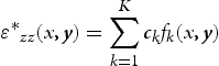
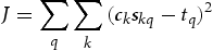
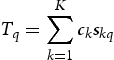
In the formulation of the inverse problem, it is first assumed that the two-dimensional spatially varying unknown eigenstrain distribution ϵ*_zz(x,y) can be expressed as a series expansion [16]: (1) where c_k represents unknown coefficients of the series terms f_k which can be created by multiplying two polynomial functions [16].

Denoted by S_k(x,y) the distribution of the axial stress component σ_zz arising from the eigenstrain given by the kth basis function f_k(x,y). Evaluating S_k(x,y) at each of the qth measurement points with coordinates (x_q, y_q) gives rise to simulated values S_kq= S_k(x_q,y_q) using each term of the function f_k. Owing to the problem's linearity, the linear combination of basis functions expressed by Equation (1) gives rise to the stress values at each measurement point given by the linear combination of S_kq with the same coefficients c_k, i.e. (2) Denoted by t_q the values of the same axial stress component at point (x_q,y_q) deduced from the experiment. To measure the goodness of the prediction, a functional J was given by the sum of squares of differences between actual measurements and the predicted values: (3)

The search for the best choice of model can now be accomplished by minimising J with respect to the unknown coefficients, c_k, i.e. by solving: (4)

The partial derivative of J with respect to the coefficient c_k can be written explicitly as: (5)

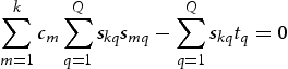
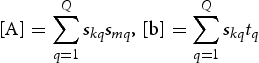
Introducing the following matrix: (6) The solution of the inverse problem has thus been changed to the solution of the above linear system for the unknown vector of coefficients c_k: (7)

In the present study, the stresses at the points within the region with a diameter of 7.2 mm are used as the finite number of residual stress component values t_q. In addition, the surface stresses at several points measured by the XRD method are also included in the experimental results to deduce the eigenstrain strain distribution responsible for the stress in the z-direction. The schematic diagram of the experimental stress used to construct the eigenstrain strain distribution is shown in Figure 3.

Figure 3

Schematic diagram of the experimental data used to find the eigenstrain distribution.

The Chebyshev Polynomials was chosen as the basis function of the eigenstrain distribution in the radial and hoop directions. The motivation for choosing the set of Chebyshev polynomials comes from the fact that they are frequently used in least-square fitting algorithms.

The higher order of polynomials was chosen to ensure good approximation to the experimental data while avoiding excessive oscillations associated with high order polynomial interpolations. The order of the polynomials has effects on the reconstructed stress distribution, and the effect of the order of the polynomial on the stress is discussed in the next section. In the present study, the same order was used for the basis function in the two directions.

Results and discussion

Stress results measured by CM and constructed by eigentrain method

The measured stress distributions on the cut plane with the CM are shown in Figure 4(a,b). The measured stress is in the direction normal to the cut plane, that is, the z-direction stress (axial stress). The stress constructed by the eigenstrain method is shown in Figure 4(c).

Figure 4

Residual stress distribution on the cut plane: (a) CM measurement; (b) CM measurement with steel block attached; (c) reconstructed stress distribution with the eigenstrain method.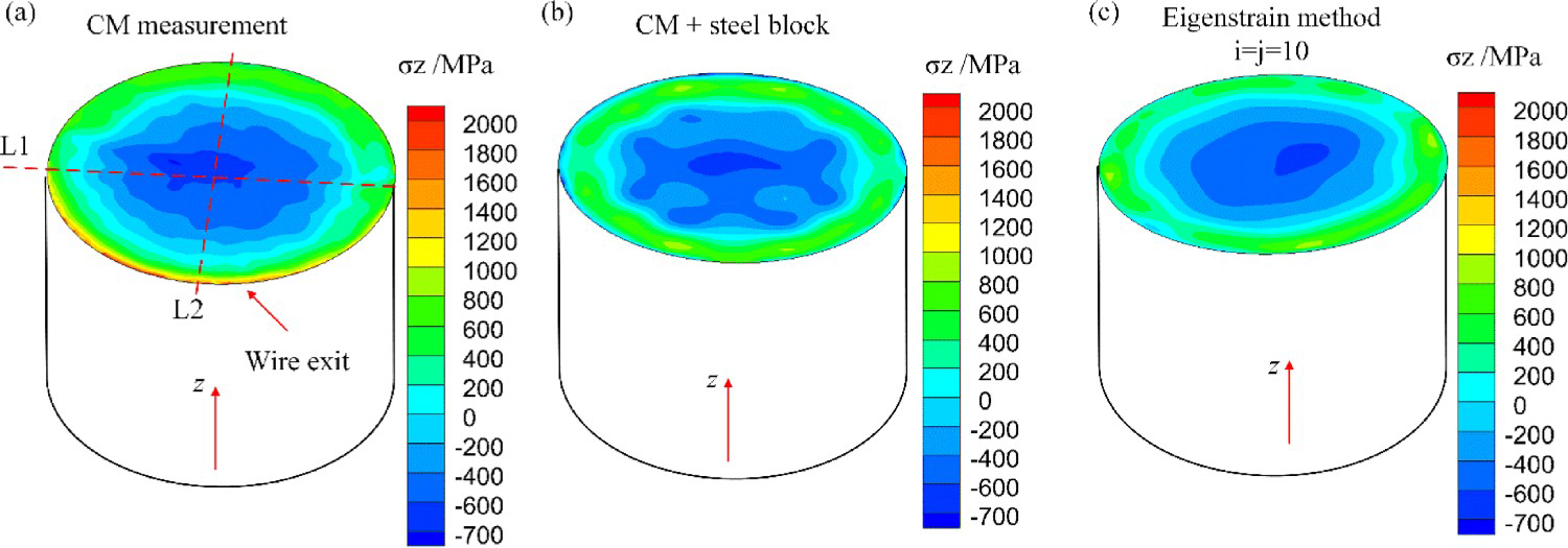

As shown in Figure 4, the axial stress in the specimen obtained by three methods show a trend of tensile exteriors and compressive interiors. The same axial stress distribtution trend is also found in a PBF additively manufactured cylindrical Inconel 625 specimen measured by neutron diffraction [18]. Ahmad et al. [10] adopted the contour method and numerical simulation method to investigate the stresses along the build direction in blocks manufactured by the PBF method. The presence of high tensile residual stresses at and near the surface of both titanium and Inconel alloys blocks was also found, whereas compressive residual stresses were seen at the centre region.

As seen from Figure 4(a), large tensile stress occurs at the edge of the wire exit side, with a peak value over 2000 MPa, which is much larger than the tensile strength of the specimen (about 1000 MPa). The surface stresses measured by the XRD at several points range from 80 MPa to 110 MPa, with an average value of 85 MPa. Therefore, a large error appears at the edge of the round-rod specimen if using CM measurement without any strategy to mitigate the displacement error at the edge.

Figure 4(b) demonstrates the stress in the specimen attached with two steel blocks before cutting to avoid the displacement error on the edge, and it is found that the tensile stress at the edge drops sharply as compared with those near the surface. Considering the low tensile surface stress measured by the XRD method (85 MPa), it can be concluded that the method by attaching steel block to the round-rod specimen for CM stress measurement can lower the measurement error at the edge to a certain extent. From Figure 4(c), the surface stress obtained by the eigenstrain method ranges from 0 to 100 MPa, which matches the results measured by the XRD. It means the stress error at the edge of the round-rod specimen can be corrected by the eigenstrain method.

From Figure 4, the stresses in the interior of the three conditions have a similar distribution; compressive stress appears in most regions inside the specimen with a peak value of about −700 MPa.

The stresses along two lines (L1 and L2 in Figure 4(a)) are shown in Figure 5. As shown in Figure 5, The stresses obtained by the three methods (CM, steel block + CM, eigenstrain method) have a very close distribution in the internal region. The stresses in the region from the centre to the diameter of about 6 mm are compressive, with a peak value of about −700 MPa appearing at the core location of the specimen. Tensile stress appears within the surface layer with a depth of 0-2 mm from the surface. However, the stresses within the surface layer (about 0.5 mm depth from the surface) are different; the surface stresses obtained by the CM are larger. Those obtained by the eigenstrain method and by attaching steel blocks drop drastically as compared with that from the CM. Peak tensile stress obtained by the eigenstrain method is about 900 MPa, which is close to the yield strength of the material and occurs at a depth of about 0.5 mm from the surface. The surface stress obtained by the eigenstrain method is about 85 MPa, which is almost the same as the results obtained by the XRD method. While the surface stress in the specimen with attaching steel blocks is compressive stress or small tensile stress. It means a large error also occurs in the surface stress of the specimen, even attaching steel blocks to reduce the displacement error of the CM. The error may be induced by the different electric conductivities of the specimen, the conductive adhesive, and the steel. The tightness between the steel blocks and the specimen also affects the cutting quality at the edge of the specimen. The EDM wire breakage occurs easily during cutting the region between the steel block and the specimen, resulting in surface waviness as shown in Figure 2(c).

Figure 5

Stress distributions along lines: (a) L1; (b) L2.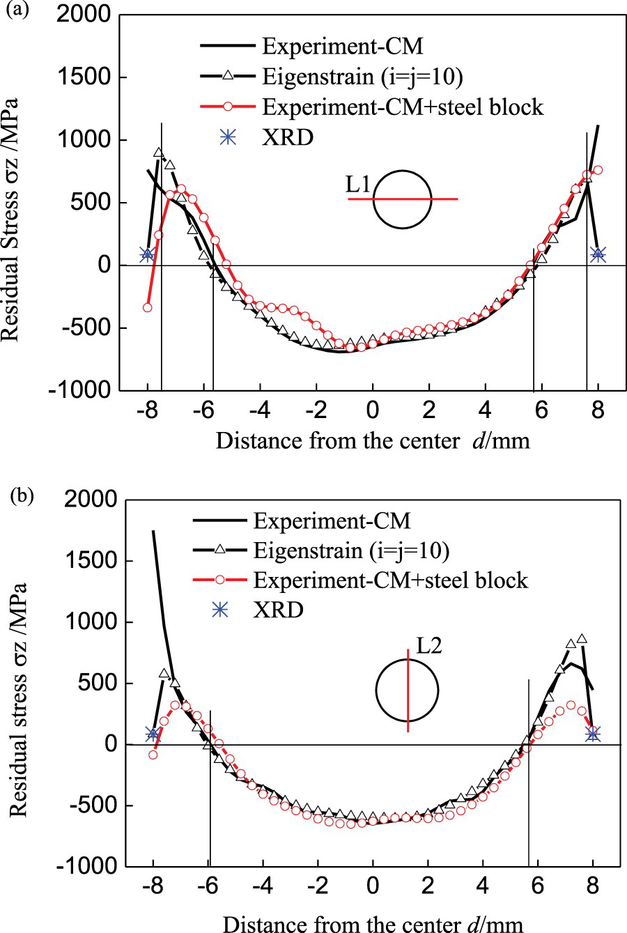

Effect of the polynomial order on the constructed stress

For the eigenstrain method to reconstruct the stress distribution, higher order of the polynomials can ensure good approximation to the experimental data, however, it could take a long time to perform the computations. There is an optimal order of the selected polynomials to get the surface stress matching the XRD results and reasonable computation time.

Several computations were carried out on different orders of the Chebyshev polynomials, the stress results were compared with each other and the XRD measurement. Figure 6 shows the results obtained by eigenstrain method using different orders of polynomials.

Figure 6

Stress distribution obtained by eigenstrain method using different polynomial orders.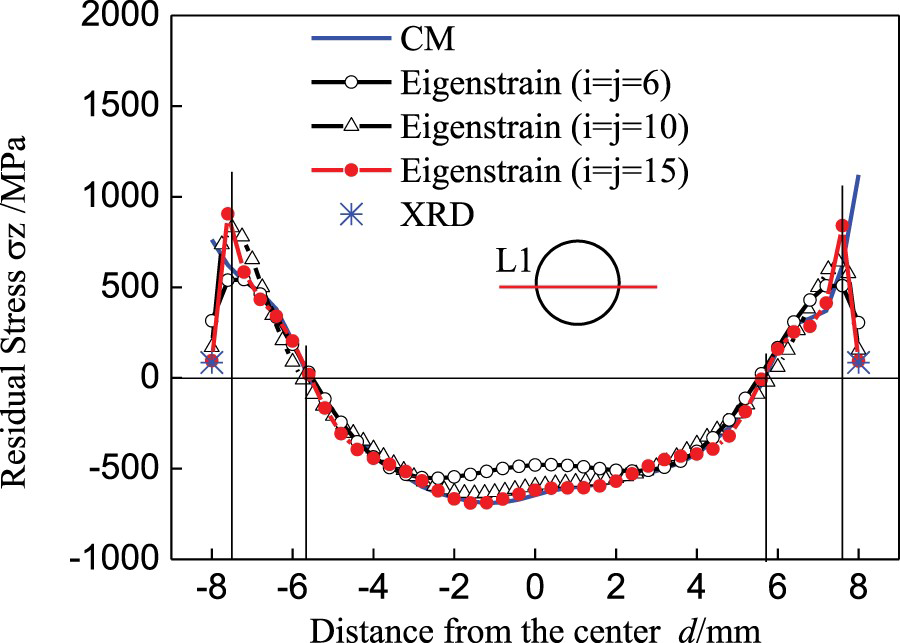

As seen in Figure 6, the higher order of the polynomials can get closer results to the surface stress obtained by the XRD method and the internal stress measured by the CM. While the stress results from the polynomials with an order of 15 are much close to those with an order of 10. Therefore, for the specimens investigated in the present study, the eigenstrain method using the Chebyshev polynomial with an order of 10 can reduce the displacement error of the CM at the edge and the corrected results agree well with the surface stress measured by the XRD. Considering the computation time and precision, the trial calculations for similar applications using eigenstrain method can start from 10-order Chebyshev polynomial.

Conclusions

The titanium alloy round-rod specimens were prepared by laser-based power-bed fusion (L-PBF) additive manufacturing and the axial stresses in these specimens were measured with the contour method. Two strategies to correct the displacement error of contour method are investigated. The main conclusions can be drawn as follows.

The axial stress in the Ti6Al4V specimen fabricated by L-PBF is tensile stress within the surface layer with a distance of about 0–2 mm from the surface, and the compressive stress occurs in most regions in the interior. The peak value of the compressive stress is about −700 MPa, which appears at the core location of the specimen.

Without correction, the peak tensile stress occurs at the surface with a magnitude much higher than the yield strength of the material. After correction, the tensile stress peak value is about 900 MPa, which is close to the yield strength of the material and occurs at a depth of about 0.5 mm from the surface. The corrected surface stress is close to that obtained by the XRD method.

Both the method of attaching steel block and the stress reconstruction method based on eigenstrain can improve the measurement accuracy of the CM on the surface layer stress to a certain extent. However, the conductivity of the conductive adhesive and the tightness between the glued steel block and the specimen affect the cutting process and would cause new test errors.

The stress reconstruction method based on eigenstrain requires accurate surface stress results and the optimisation of the order of the eigenstrain basis function.

Footnotes

Disclosure statement

No potential conflict of interest was reported by the author(s).

References

Herzog

, Seyda

, Wycisk

, Additive manufacturing of metals. Acta Mater. 2016; 117:371–392. doi:10.1016/j.actamat.2016.07.019.

Zhang

, Zhou

, Energy absorption diagram characteristic of metallic self-supporting 3D lattices fabricated by additive manufacturing and design method of energy absorption structure. Int J Solids Struct. 2021; 226–227:111082. doi:10.1016/j.ijsolstr.2021.111082.

, Pan

, Ding

, A review of the wire arc additive manufacturing of metals: properties, defects and quality improvement. J Manuf Process. 2018; 35:127–139. doi:10.1016/j.jmapro.2018.08.001.

Biegler

, Elsner

BAM

, Graf

, Geometric distortion-compensation via transient numerical simulation for directed energy deposition additive manufacturing. Sci Technol Weld Joining. 2020; 25(6):468–475. doi:10.1080/13621718.2020.1743927.

Withers

PJ.

Residual stress and its role in failure. Rep Prog Phys. 2007; 70(12):2211–2264. doi:10.1088/0034-4885/70/12/R04.

Prime

MB.

Cross-sectional mapping of residual stresses by measuring the surface contour after a cut. J Eng Mater Technol. 2001; 123(2):162–168. doi:10.1115/1.1345526.

Martina

, Roy

, Szost

, Residual stress of as-deposited and rolled wire +arc additive manufacturing Ti–6Al–4V components. Mater Sci Technol. 2016; 32(14):1439–1448. doi:10.1080/02670836.2016.1142704.

, Brown

, Kumar

, An experimental investigation into additive manufacturing-induced residual stresses in 316L stainless steel. Metall Mater Trans A. 2014; 45(13):6260–6270. doi:10.1007/s11661-014-2549-x.

Moat

, Pinkerton

, Li

, Residual stresses in laser direct metal deposited Waspaloy. Mater Sci Eng A. 2011; 528:2288–2298. doi:10.1016/j.msea.2010.12.010.

10.

Ahmad

, van der Veen

, Fitzpatrick

, Residual stress evaluation in selective-laser-melting additively manufactured titanium (Ti-6Al-4V) and inconel 718 using the contour method and numerical simulation. Addit Manufact. 2018; 22:571–582. doi:10.1016/j.addma.2018.06.002.

11.

Hatamleh

, DeWald

An investigation of the peening effects on the residual stresses in friction stir welded 2195 and 7075 aluminum alloy joints. J Mater Process Technol. 2009; 209(10):4822–4829. doi:10.1016/j.jmatprotec.2008.12.010.

12.

, Wu

, Withers

, The effect of manufacturing defects on the fatigue life of selective laser melted Ti-6Al-4V structures. Mater Des. 2020; 192:108708. doi:10.1016/j.matdes.2020.108708.

13.

Hosseinzadeh

, Kowal

, Bouchard

PJ.

Towards good practice guidelines for the contour method of residual stress measurement. Journal of Engineering. 2014; 2014(8):453–468. doi:10.1049/joe.2014.0134.

14.

Olson

, DeWald

, Prime

, Estimation of uncertainty for contour method residual stress measurements. Exp Mech. 2015; 55(3):577–585. doi:10.1007/s11340-014-9971-2.

15.

Toparli

, Fitzpatrick

ME.

Development and application of the contour method to determine the residual stresses in thin laser-peened aluminum alloy plates. Exp Mech. 2016; 56:323–330. doi:10.1007/s11340-015-0100-7.

16.

Korsunsky

, Regino

, Nowell

Variational eigenstrain analysis of residual stresses in a welded plate. Int J Solids Struct. 2007; 44(13):4574–4591. doi:10.1016/j.ijsolstr.2006.11.037.

17.

Kartal

, Kang

Y-H

, Korsunsky

, The influence of welding procedure and plate geometry on residual stresses in thick components. Int J Solids Struct. 2016; 80:420–429. doi:10.1016/j.ijsolstr.2015.10.001.

18.

Bass

, Milner

, Gnäupel-Herold

, Residual stress in additive manufactured nickel alloy 625 parts. J Manuf Sci Eng. 2018; 140(6):061004. doi:10.1115/1.4039063.