Results of an international round-robin exercise on electrochemical impedance spectroscopy

Abstract

ABSTRACT

To check the reproducibility of electrochemical impedance spectroscopy (EIS) measurements, 19 laboratories have performed round-robin (RR) testing on EIS using various instruments and three different systems: a dummy cell and two electrochemical systems of practical interest in the nuclear corrosion domain. The general conclusion drawn from the tests performed with the dummy cell is that the actual commercially available instruments for EIS measurements are suitable to produce good quality data. Differences in the EIS diagrams for the tested electrochemical systems were observed and discussed. This RR exercise, involving for the first time a large number of laboratories, shows that intrinsic scatter (large or small) is present in the impedance data and that reproducibility should be readily checked. While EIS is an excellent technique for investigating the kinetics of electrochemical systems, great care has to be taken on planning and conducting the experiments. Recommendations are given to help obtaining reliable EIS results.

Keywords

Electrochemical impedance spectroscopy round-robin test dummy cell corrosion

Introduction

The European Cooperative Group on Corrosion Monitoring of Nuclear Materials (ECG-COMON, www.ecg-comon.org) was established in 2004 with the main aim to improve corrosion monitoring techniques and equipment to be used for structural materials in nuclear and other industrial environments. One of the activities to accomplish this goal is the annual organisation of a round-robin (RR) exercise for the involved laboratories. A first series of RRs was related to the electrochemical noise (EN) technique. The published results show rather large deviations between the power spectral densities of the potential and current time records measured by the different laboratories and equipment on dummy cells and electrochemical systems, even when using a dedicated test procedure [1,2]. A second series of RR tests was organised on the electrochemical impedance spectroscopy (EIS) technique. As for the EN RRs, a detailed test procedure has been set up by the group and used by the participants to test different systems. The principles and results are presented below after a short introduction of the EIS technique.

In the EIS technique, a small sinusoidal potential or, less commonly, current signal of a certain frequency is used to perturb the electrochemical system around the polarisation point investigated. The current or potential response is measured and the modulus and phase shift of the impedance are determined [3 7]. Information on electrochemical corrosion phenomena are then obtained in situ, so that EIS appears as a non-destructive technique and, therefore, a good candidate for monitoring corrosion processes. Three conditions are required to obtain valid EIS experimental data: (1) stability, (2) linearity and (3) causality of the system [6]. Stability means that the system comes back to its initial state after superposition of a small and short perturbation signal. So, by using a small potential or current perturbation signal, the system is expected to stay close to its steady state in the linear region, in which the amplitude of the system response is proportional to that of the perturbation signal. On the other hand, causality means that the system response is induced by the perturbation signal, which is fulfilled for stationary systems with small background noise. Stationarity means that the system remains in the same state during the experiment. Satisfying this requirement is sometimes difficult, since a corroding system is often changing with time. For slow changes, the system is assumed to be quasi-stationary and valid experimental data can be obtained. For the difficult, but fortunately not too frequent, cases of electrochemical systems not respecting the basic conditions required for EIS measurement, advanced signal processing or instrumental techniques have been proposed in the literature [8 10].

Under circumstances where a standard reference electrode cannot be used (e.g. for light water reactor type or research investigations in autoclave experiments at high temperature and pressure) EIS measurements can also be performed with a pseudo-reference electrode, like a Pt wire. But great care should be taken when analysing such EIS measurements. Although there is no widespread application currently, some works have already been carried out on stainless steels and Ni-based alloys in high-temperature and high-pressure autoclaves [11 13].

The present RR testing on EIS has been carried out with the main aim to check the reproducibility of EIS measurements performed at ambient temperature by different laboratories and equipment. This paper does not intend to consider the applications of EIS to the study of electrochemical processes, nor recent progresses in EIS analysis (the reader is referred to the extensive available literature on these topics [3 7,14,15]). Instead, it focuses on the principles of the measurement process and the analysis/validation of such measurements. While several standards about EIS have been published [16 18], to the best of our knowledge, no EIS RR test with a substantial number of participants (>3) has been reported, only one was presented recently at an EIS conference [19]. Therefore, a series of RR exercises have been undertaken by the ECG-COMON to evaluate to which extent the equipment and laboratory lead to comparable results, as is the aim of an RR. Three trials were performed. In the first one (RR1), EIS measurements were carried out on a dummy cell consisting of a circuit of resistors and capacitors with typical values for electrochemical systems in the corrosion domain. This allowed primarily the different electronic devices used for EIS measurements to be checked. Indeed, it is important to note that all EIS equipment have various limitations in their characteristics, for example, in the measurement frequency bandwidth, at high and low frequencies, and in the input impedance, i.e. the maximum and minimum measurable impedance. In the following trials, because most participants are working in the nuclear corrosion field, it was decided to select electrochemical systems of practical use in this domain or which already have been investigated by some of them. In the second trial (RR2), Cu in CuSO₄ solution was studied. Because of the large deviation in results of the second trial, this RR exercise was repeated with an improved set of guiding notes. In the third trial (RR3), Zr in Na₂SO₄ solution was selected showing impedances with a magnitude exceeding 1 MΩ.

This paper summarises the results of all three RR exercises, focusing primarily on problems that were experienced during testing and the limitations of various measurement systems. A total of 19 laboratories participated to this study, using 23 measurement systems, including mainly general-purpose potentiostats and frequency response analysers (FRAs) from different manufacturers: Bio-Logic [SP-200 (1)], Gamry [Ref600 (8), PC3/750 (1), PCI4/750 (2), PCI4/300 (1), Interface 1000 (1)], Ivium Technologies [Compactstat (1)], IPS Elektroniklabor GmbH & Co. KG [IPS PGU 10V-1A-IMP-S (1)], Metrohm [Autolab PGSTAT302N + FRA32M (1)], Solartron [1260 FRA + 1287 potentiostat (1), 1255B FRA + 1287a potentiostat (2), Modulab (1), 1250 FRA + Macrostat MGS-03 (homemade potentiostat) (1)], Zahner [IM6e (1)]. The equipment used in each laboratory is not identified in the paper for reasons of confidentiality.

Experimental

Three different systems were used: a dummy cell and two electrochemical systems (Cu/CuSO₄ and Zr/Na₂SO₄). A summary of the experimental procedures for the RR exercises is presented in the Appendix. Note that it was recommended to switch the EIS measuring device to the shortest measurements procedure available to have a standard measurement setup for all measurement devices, some of them having no possibility to increase the integration time of the signals during the impedance measurement. Moreover, the electrochemical systems investigated were not expected to generate electrochemical noise of large amplitude implying long integration times. Note also that a very large measurement frequency bandwidth was defined in the testing procedure, 0.1 mHz for the dummy cell to investigate the limits of the measuring instruments, and 0.5 or 1 mHz for the electrochemical systems to analyse the largest possible frequency bandwidth, even if frequencies below 10 mHz are rarely used in corrosion investigations. The procedures, as well as the dummy cells and working electrodes, were sent to all participants by a single organisation (SCK CEN) since this is a key definition of the RR tests that must be performed by all participants under the same conditions. Finally, not all 19 laboratories participated in all RR campaigns, the number of laboratories participating to each campaign being mentioned in the figures (14 participants in RR1, 13 in RR2 and 10 in RR3).

Part 1: Dummy cell

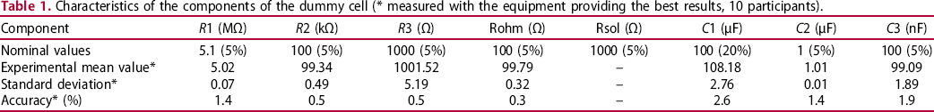
A dummy cell has been constructed, consisting of a number of resistors and capacitors with values ranging from low to high impedances and a wide range of time constants. A photograph and a schematic of this dummy cell are shown in Figure 1. The values of the resistors and capacitors are summarised in Table 1. They were chosen to mimic typical impedances in the corrosion domain but limiting the highest resistance value to 5 MΩ because some measuring devices are unable to measure impedances of higher magnitude; this allowed testing more equipment in RR1. Spreading in the results should, in the ideal case, be small, but can exist due to the use of different equipment, differences in testing environment (background noise), etc. Two tests without and two tests with Faraday cage were carried out according to the procedure described in the Appendix.

Figure 1

(a) Dummy cell used in RR1 and (b) electric scheme. The value of each component is given in Table 1.

Table 1

Characteristics of the components of the dummy cell (* measured with the equipment providing the best results, 10 participants).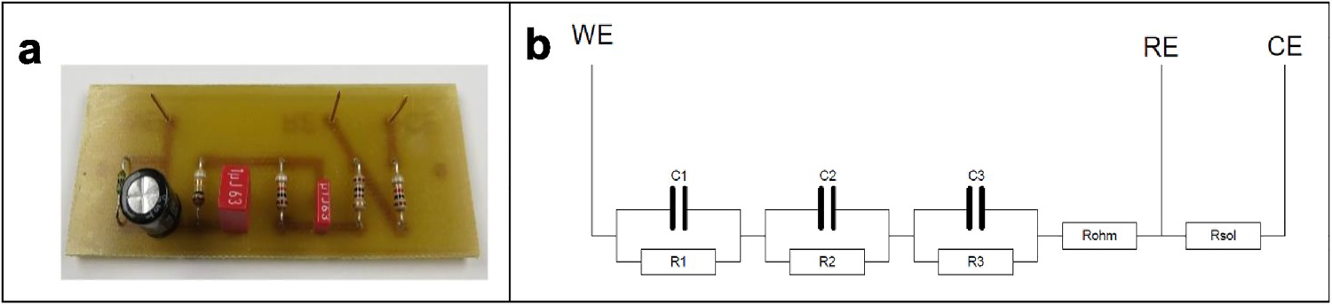

Component	R1 (MΩ)	R2 (kΩ)	R3 (Ω)	Rohm (Ω)	Rsol (Ω)	C1 (μF)	C2 (μF)	C3 (nF)
Nominal values	5.1 (5%)	100 (5%)	1000 (5%)	100 (5%)	1000 (5%)	100 (20%)	1 (5%)	100 (5%)
Experimental mean value*	5.02	99.34	1001.52	99.79	–	108.18	1.01	99.09
Standard deviation*	0.07	0.49	5.19	0.32	–	2.76	0.01	1.89
Accuracy* (%)	1.4	0.5	0.5	0.3	–	2.6	1.4	1.9

Parts 2 and 3: Electrochemical systems

The electrochemical system used in RR2 consisted of a Cu wire in 1 M CuSO₄ solution. This system is frequently used as a reference electrode in field experiments because its reaction kinetics is fast and thus this electrode is considered as non-polarisable. The electrochemical system used in RR3 consisted of a Zr wire in a 0.5 M Na₂SO₄ solution. The Zr wire oxidises over time forming a passive oxide layer which has a very poor electric conductance and so a very high resistance.

In RR2, the working electrode (WE) and counter electrode (CE) were made of a 1 mm diameter Cu wire (99.95% purity) used as-received without surface treatment. In RR3, the WE was made of a 1 mm diameter Zr wire (99.95% purity), while the CE was made of a Pt wire or mesh (as an alternative, a stainless steel wire could be used). The surface treatment of the WE consisted of wet polishing with 2500 SiC paper, rinsing with demineralised water, and then immediate immersion in the test solution.

The cell configuration was similar in RR2 and RR3, as shown in Figure 2(a,b). The WE consisted of the wire bent to a 3 cm diameter circle around the reference electrode (RE) and the CE of a 9 cm diameter circle around the RE. When possible, the vertical part of the wires was masked-off by PTFE tape or by heat-shrinkable PTFE tube, or silicone sealant, etc. The WE electrode was immersed in the solution 3 cm deep, i.e. the total wire length that was soaked in the solution was 10 cm (surface area ≈ 3 cm²). The distance of the CE below the WE was not specified in the test procedure. A commercial Ag/AgCl electrode (without Haber-Luggin capillary) was used as RE and placed in the centre of the Cu and Zr wire circles. The system was open to the air (no gas purging) and at room temperature.

Figure 2

Schematics of the (a) Cu/CuSO₄ and (b) Zr/Na₂SO₄ electrochemical cells.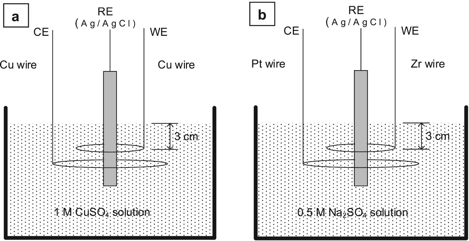

The participants in the RR tests were invited to perform:

three impedance measurements in RR2, one under galvanostatic control and two under potentiostatic control,

seven impedance measurements under potentiostatic control in RR3,

according to the procedure shown in the Appendix to study the influence of the time of exposure in solution and of the amplitude of the excitation signal used in RR3.

Reporting and analysis

The raw EIS data were collected by the participants in ASCII files that were sent to SCK CEN. These files were analysed in Excel and Origin with simple macros to obtain Nyquist and Bode plots of the various results. The results collected in this way were quite consistent, although sometimes the frequency range used for testing deviated from the test procedure, i.e. the start frequency was lower and/or the end frequency was higher. In a few cases, the imaginary part of the impedance was recorded as a positive value for a capacitive impedance: the results were then corrected before computing the summary graphs. This was the only correction performed on the raw data, which otherwise were shown as received. No validation of the EIS data by tools, such as the Kramers–Kronig relations [5,6,15], was asked from the participants in the testing procedure, because these tools were not available by default in all instrument software.

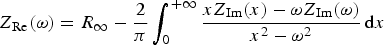
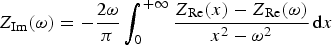
As mentioned in the introduction, stability, linearity and causality of the system are necessary conditions to obtain valid EIS experimental data. Violation of either of these conditions may be detected by using Kramers–Kronig relations that check whether the real part and the imaginary part of the measured impedance are internally consistent. These relations, based on the integration of the real or the imaginary part of the impedance over the frequency limits of zero to infinity, cannot be used directly in all situations, especially when the low-frequency and/or high-frequency limits of the impedance are not reached in the measured frequency range [15]. Different advanced data processing techniques exist for such cases to avoid the direct integration of the Kramers–Kronig relations [20 22], often requiring the existence of models (electrical circuit analogue, measurement model, etc.). In this paper, in order to test the compliance of the raw impedance data to the Kramers–Kronig relations, two different methods were used. Direct integration of the following relations: (1) (2) with obvious notations (ω = 2π f, Z _Re = Real part of Z, Z _Im = Imaginary part of Z) was performed using an in-house developed software. The second method, developed by B.A. Boukamp and called ‘indirect integration’ in this paper, is based on a linear least squares fit algorithm, using the impedance of a series connection of parallel R–C circuits (Voigt network), hence avoiding the development of electrical circuits for both electrochemical systems tested, which was beyond the scope of the round-robin exercise. The basic idea of this method is that each R–C circuit, and therefore the entire circuit, obey the Kramers–Kronig relations. So, when the raw impedance data can be fitted to the entire circuit with reasonable accuracy, then it can be considered that they obey the Kramers–Kronig relations. The executable program, equivcrt, downloadable from the Twente University website [23], was used with the default values of the Kramers–Kronig test settings, as recommended [21,24]. It is important to note that the fitted values R _k, C _k of the R–C circuits do not all have a physical meaning since they may be negative (while the time constants R _kC _k are always positive to satisfy the causality requirement).

Results and discussion

Part 1: Dummy cell

The first trial was mainly a test of the equipment as it was not expected that much could go wrong in connecting the dummy cell. Figure 3 shows the results of measurement B in the frequency range 1 MHz to 0.1 mHz, where no Faraday cage was used. With the exception of one test (red points), probably due to a bad functioning of the potentiostat or faulty electrical contact, there is very good agreement in the results of the 13 other tests. Figure 3(a) shows a low scatter at very low frequencies where the impedance magnitude is higher than 1 MΩ, with the exception of a few wrong points (orange, red and purple points). It is impossible to quantify the measurement accuracy precisely because the measurements were performed in different laboratories, therefore using different dummy cells with resistors and capacitors of precision 5 and 20%, as shown in Table 1. To identify the accuracy of his EIS measuring equipment, the user is recommended to refer to the data sheet or accuracy contour plot given by the manufacturer.

Figure 3

EIS data for the dummy cell (RR1): Nyquist diagrams at (a) low frequency, (b) mid-frequency, (c) high frequency and (d) Bode plots (without Faraday cage, ΔV = 10 mV_rms, 14 participants). The solid lines correspond to the impedance simulated with the fitted values of the components given in Table 1. (a–d) Raw data, (e) data validated by direct integration with an error lower than 3%, (f) data validated by indirect integration with an error lower than 3%.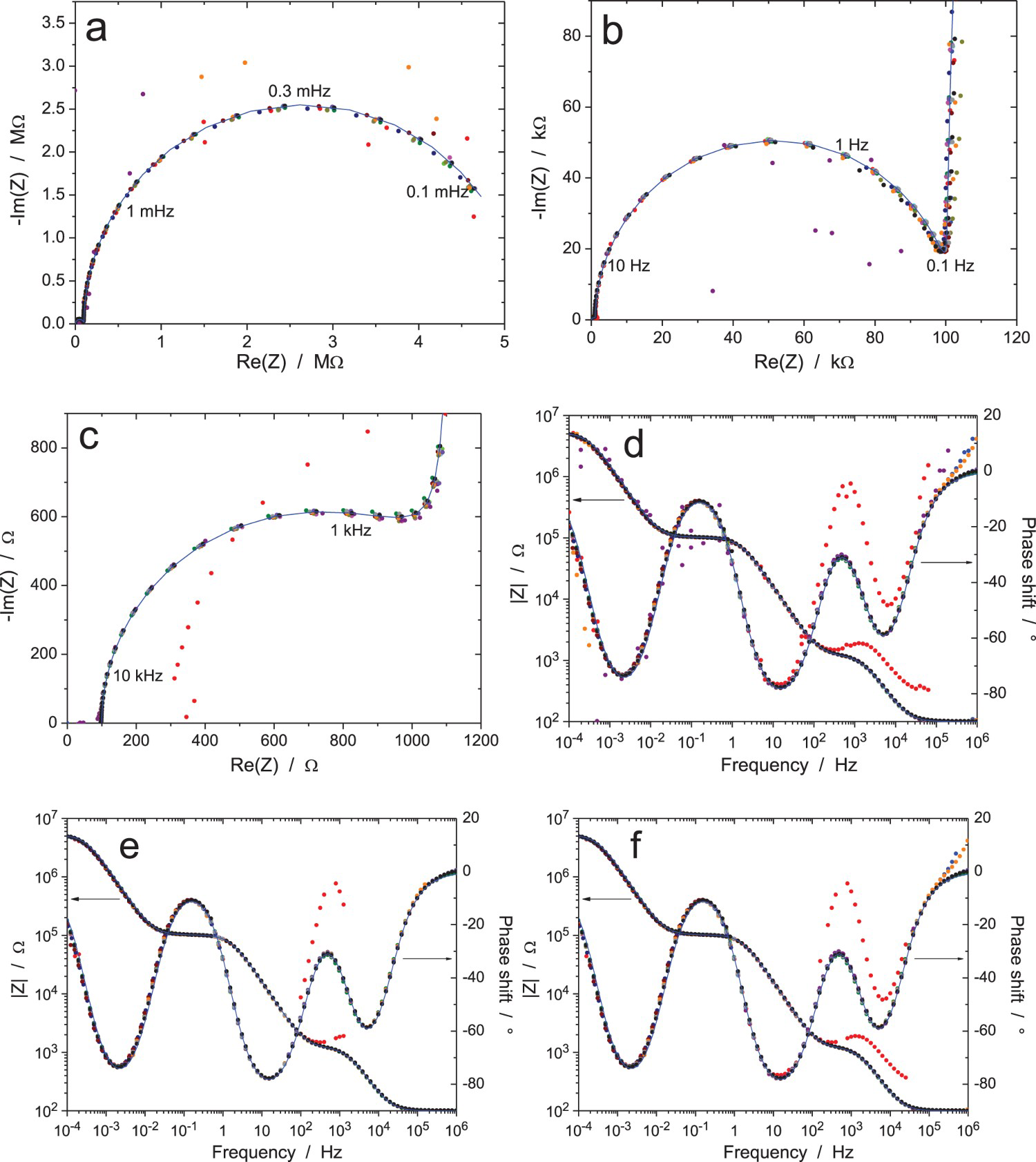

Table 1 shows that the mean value, standard deviation and accuracy of the components are in good concordance with the expected values. These results were obtained by fitting the experimental data given by the equipment providing the best results (10 participants), with the theoretical value of the impedance given by the below equation: (3) Figure 3 also shows a perfect agreement between the experimental impedance values and those calculated with the fitted values of the dummy cell components (solid lines). Measurements with a Faraday cage to shield against external noise sources were also performed by some participants. No significant improvement of the measurement impedance was obtained. It can also be noted that some instruments did not give correct impedance values above 100 kHz (see Figure 3(d)). Some of the participants even tried to measure the impedance at frequencies higher than 1 MHz, but without success. For electrochemical systems, however, frequencies above 100 kHz or 1 MHz are of limited interest, so this is not a key issue. In conclusion, all the potentiostats but one performed well with the dummy cell in the frequency range from 100 kHz to 0.1 mHz.

Even if it is not necessary to check the compliance of the raw data to the Kramers–Kronig relations, in this case where the theoretical impedance curves are given in Figure 3(a–d), direct and indirect integrations were performed. Figure 3(e,f) shows the Bode diagrams of the impedance data validated, respectively, by direct and indirect integration with an error lower than 3%. This validation error is defined as follows: (4) where (Z _Re, Z _Im) and (Z _Re,valid, Z _Im,valid) concern, respectively, the measured impedance and the impedance validated by either direct or indirect integration. It can be seen in Figure 3(e,f) that all scattered points in Figure 3(d) have been eliminated by both validation processes. Some slight differences in these processes can be mentioned, first on the outlier data represented by the red curve and second above 100 kHz where indirect integration validates obviously incorrect points (negative phase angle), in contrast to direct integration. This might be due to a too large number of R–C circuits leading to over-fitting. This indirect integration problem was addressed in Ref. [22]. Results in direct integration also depend on the choice of the immittance (impedance or admittance) and of the impedance component (real or imaginary part) submitted to the Kramers–Kronig criterion. It is recommended to integrate the admittance (resp. impedance) for measurements under potentiostatic (resp. galvanostatic) mode in order to systematically analyse the transfer function ‘response/excitation’ [25]. It should also be mentioned that when the impedance diagram does not reach its low-frequency limit in the measured frequency range, as in Figure 3(a) or for the Zr/Na₂SO₄ system, direct integration from frequency zero is not possible. In that case, it is better to use the admittance since its Nyquist diagram converges to the real axis at high and low frequencies, and, therefore, this gives better integration results. The best results in Figure 3(e) were obtained by integrating the real part of the admittance [Equation (2) with 1/Z instead of Z].

Part 2: Cu/CuSO₄ electrochemical system

This trial was carried out in two steps. The first one, performed under potentiostatic control at the open circuit potential (OCP), showed that the system was very sensitive to the amplitude of the voltage perturbation, ΔV. This is illustrated in Figure 4(a) in which the inductive loop disappeared only for amplitudes of ΔV <5 mV_rms, indicating that the polarisation curve is far from being linear around the OCP. Moreover, indirect integration performed on the raw data shows that the major part of the impedance diagrams for ΔV = 10 and 20 mV_rms are not validated in Figure 4(b) due to drifting current responses (see below). This is after all not surprising as the Cu/CuSO₄ electrochemical system is considered as ‘non-polarisable’ and can be used as a reference electrode [26]. Therefore, in the second round, the amplitudes of the voltage excitation were fixed to 0.1 and 1 mV when working under potential control at OCP, and a galvanostatic test at zero DC current was added to avoid over-polarisation of the electrochemical system. The results of the second test campaign are presented in Figures 5–7, in which each data with the same colour have been measured by the same participant.

Figure 4

Influence of the perturbation amplitude, ΔV _rms, on the impedance of the Cu/CuSO₄ system measured by a single participant in potentiostatic mode, sequentially with small to large ΔV _rms value. Frequencies in Hz (lowest frequency 10 mHz). (a) Raw data, (b) data validated by indirect integration with an error lower than 3%.

Figure 5

EIS raw data for the Cu/CuSO₄ system (RR2, measurement A: immersion time 1 h, ΔI = 10 µA_rms): (a) Nyquist diagram; (b) enlargement around the origin; (c and d) Bode plots (13 participants).

Figure 6

EIS raw data for the Cu/CuSO₄ system (RR2, measurement B: immersion time 5 h, ΔV = 0.1 mV_rms): (a) Nyquist diagram; (b) enlargement around the origin; (c and d) Bode plots (10 participants).

Figure 7

EIS data for the Cu/CuSO₄ system (RR2, measurement C: immersion time 9 h, ΔV = 1 mV_rms): (a and b) Nyquist diagrams and (c and d) enlargement around the origin of (a and c) raw data and (b and d) data validated by indirect integration with an error lower than 3%; (e and f) Bode diagrams of raw data (13 participants).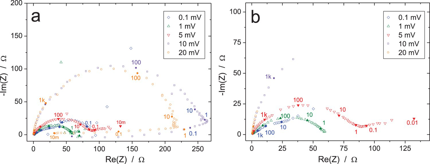

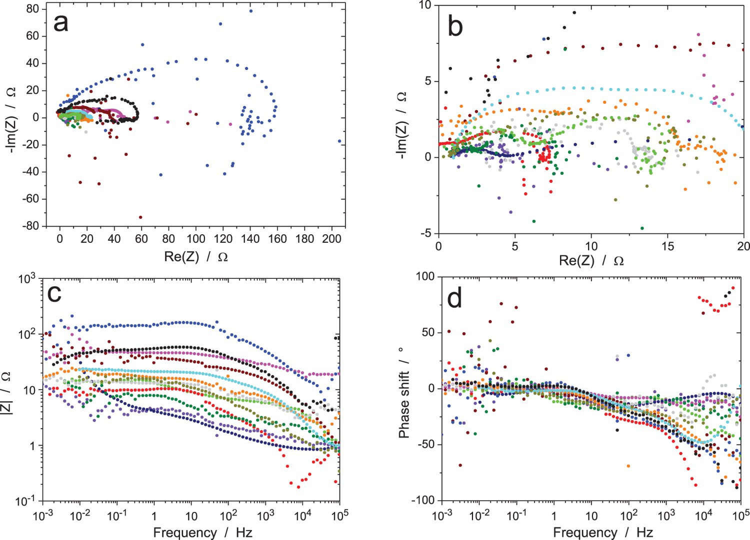
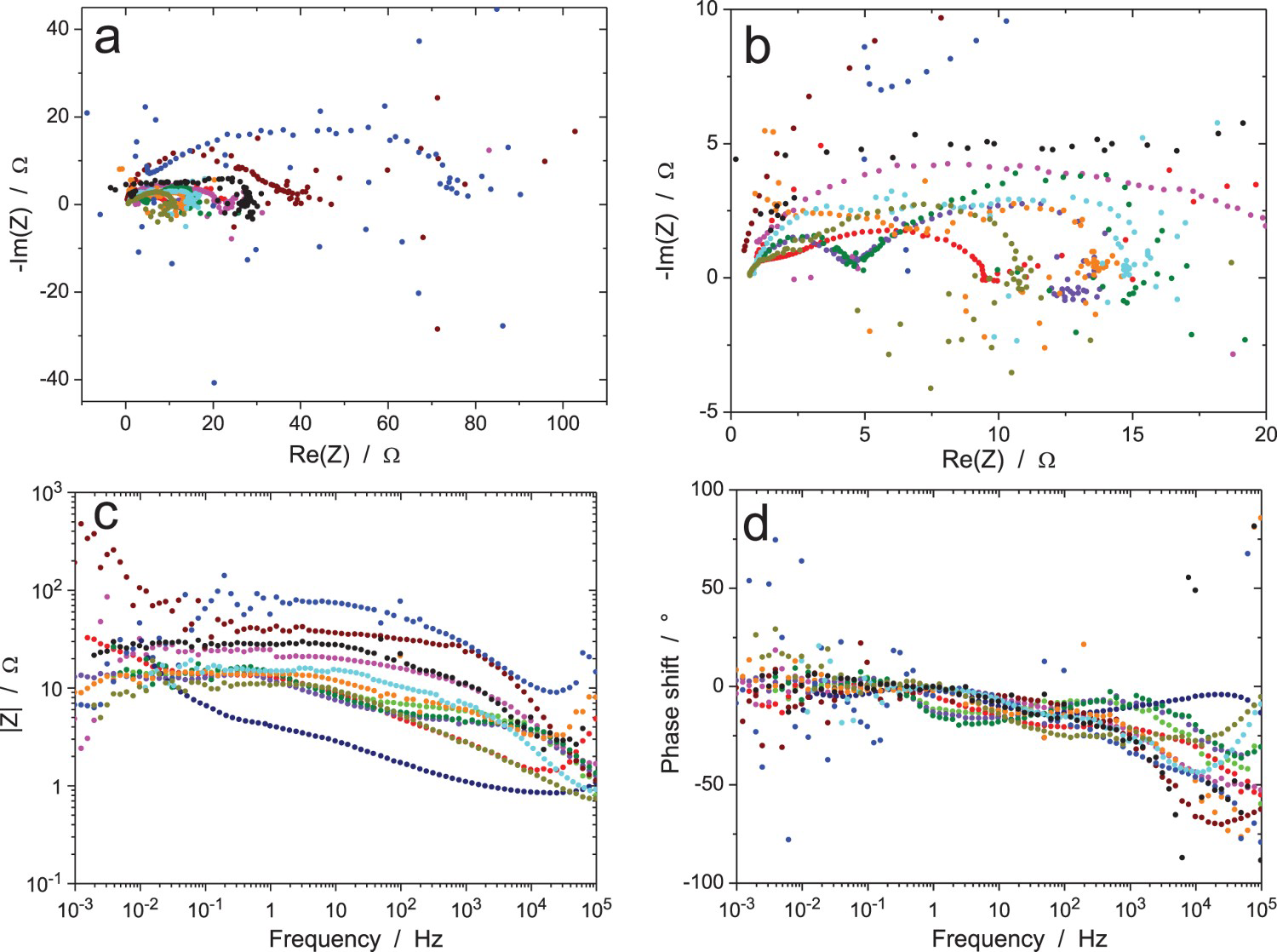
The results of the first test, which was performed under galvanostatic control (measurement A), are shown in Figure 5. While low values of the impedance modulus were measured due to the high exchange current density of the electrochemical reaction, there was a large scatter in the experimental data, with Nyquist diagrams showing different shapes and amplitudes, as well as many dispersed points mainly at low and high frequencies. This is not related to the fact that different instruments were employed since impedance moduli lower than 15 Ω or higher than 100 Ω were measured by participants using the same equipment. It could be argued that the amplitude of the current excitation (10 µA_rms) was too large, but the width of most Nyquist diagrams was lower than 20 Ω, which corresponds to a 0.2 mV_rms amplitude of the voltage response, which is rather small. The mid-frequency range showed results that seem in better agreement with each other for the phase angle, but this is mainly due to the fact that the capacitive loops in the Nyquist diagrams are depressed, hence giving low values of the phase angle.

The results of the tests performed in potentiostatic mode with an excitation signal of amplitude ΔV = 0.1 mV_rms (measurement B) are shown in Figure 6. They are very similar to those obtained in galvanostatic mode with a large scatter in the shape and amplitude of the Nyquist diagrams and many inaccurate impedance data in the low- and high-frequency ranges. This is due to the too low amplitude of the voltage excitation signal. The Bode diagrams also show measurement errors at the power-line frequency of 50 Hz and harmonics. Validation of the impedance data by direct or indirect integration was not performed for measurements A and B because of the too large measurement errors caused by the low excitation signal. Direct integration of scattered Z _Re or Z _Im values cannot give accurate results and indirect integration will tend to use a too large number of R–C circuits to better fit the dispersed data. For measurement C in potentiostatic mode with ΔV = 1 mV_rms, the results in Figure 7 are much less noisy than for measurement B because of the higher excitation signal; however, the Nyquist diagrams still show clear differences in shape and amplitude of the loops. Validation could be performed by both validation methods on these better accurate impedance data. The major part of all impedance diagrams could be validated by either method with the exception of the weird curve of largest amplitude in Figure 7(a), as shown in Figure 7(b) when using indirect integration.

In some Nyquist diagrams of the impedances measured by the participants, it is possible to see the influence of signal drift on the impedance value at low frequency (inductive loop above the X-axis or capacitive loop below the X-axis, etc.), which is not unexpected since almost all electrochemical systems are drifting with time and the participants had to measure the impedance at frequencies down to 1 mHz. When the impedance does not change significantly during the measurement time, the theoretical effect of a linear current (resp. potential) drift on the impedance in potentiostatic (resp. galvanostatic) mode is given by the following expressions [27,28]: (5) (6) where ΔV _rms (resp. ΔI _rms) is the rms amplitude of the potential (resp. current) excitation signal and a _v (resp. a _i) is the drift rate of the voltage (resp. current) response in V/s (resp. A/s), while t _o is the initial time of the calculation of the four integrals implied in the analogue lock-in ampliﬁer technique used in most FRA to determine the impedance value at frequency f. As a simple example, the effect of a linear drift of rate a _i = ±1 nA/s on the impedance of a dummy cell under potentiostatic control was calculated for an excitation signal of amplitude 10 mV_rms with Equation (5). At frequencies below 0.1 Hz, the amplitude of the drift during a period of the sine wave signal becomes more and more significant compared to the amplitude of the excitation signal when the frequency decreases, which explains the errors in the impedance diagrams presented in Figure 8. Similar results can be obtained in galvanostatic regime from Equation (6).

Figure 8

Influence of a linear drift on the impedance of a dummy cell (r + (R//C)) with r = 10 Ω, R = 10 kΩ, C = 150 µF in potentiostatic regime (ΔV _rms = 10 mV, a _i = 1 nA/s) from Equation (2) with t _o = 0. Frequencies in Hz.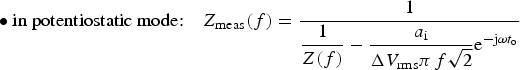

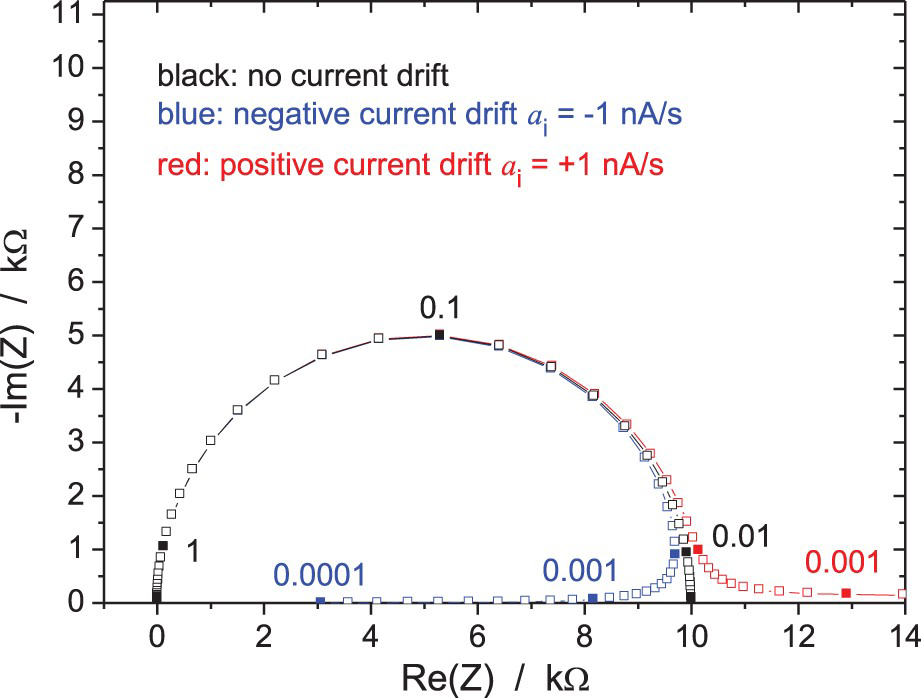
When the impedance varies significantly during its measurement, the problem is much more involved. The low-frequency points in the Nyquist diagram tend to move too, but in that case, the direction of that movement also depends on the fact that the impedance increases/decreases and on the frequency sweep mode (ascending or descending). This drift problem can be partly solved when the FRA and potentiostat/galvanostat are two different instruments by inserting an analogue high-pass filter between them, the cut-off frequency of the filter being controlled to be lower than the measured frequency. However, this is not possible for most modern instruments containing both potentiostat/galvanostat and FRA in the same box. A solution could be the implementation by the manufacturers of digital high-pass filtering on both, potential and current channels in their equipment.

In conclusion, for the Cu/CuSO₄ system, the RR tests showed large deviations in the results of the participants, even if some of them are quite acceptable, as those given in Figure 9. It could be mentioned that the deviations might be due to differences in the assembly of the electrochemical cells, in particular because the position of the CE was not specified in the measuring procedure so that the position of the RE was not always between the WE and CE, as usually recommended. But it is important to mention that measuring the impedance of the Cu/CuSO₄ system is a difficult task due to its ‘non-polarisability’, as mentioned above. It requires using excitation signals of very low amplitude so that the system is more prone to be influenced by external noise sources. In principle, galvanostatic mode with a mean current of zero should be the best way for measuring the impedance of a reference electrode, because the mean voltage is not a priori prone to vary with time. Unfortunately, the amplitude of the excitation current signal was chosen too low to get accurate results in Figure 5. This system could be considered as not adequate for performing an RR test, but it can also be considered that the exercise better illustrates the care that must be taken when measuring the impedance of an electrochemical system.

Figure 9

Nyquist diagrams of the EIS raw data for the Cu/CuSO₄ system (RR2, measurements A: immersion time 1 h, ΔI = 10 µA_rms, B: immersion time 5 h, ΔV = 0.1 mV_rms and C: immersion time 9 h, ΔV = 1 mV_rms): influence of the immersion time and amplitude of the voltage excitation for two participants (a and b), using the same equipment. Frequencies in Hz.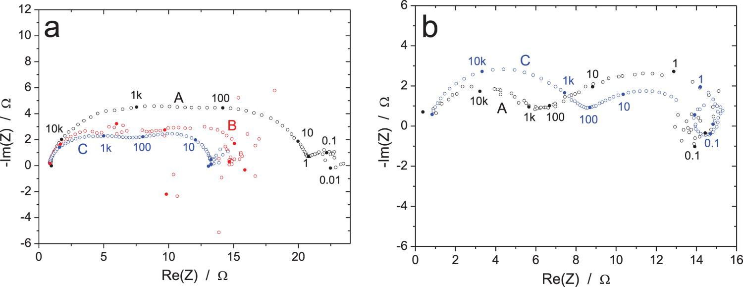

Part 3: Zr/Na₂SO₄ electrochemical system

The third trial consisted of a Zr wire immersed in a sodium sulphate solution, which had as a consequence that the wire surface oxidised over time forming a thicker passive layer. This means that with each successive measurement, the magnitude of the impedance was increasing. However, this change in impedance was fast only during the first few hours and then slowed down rapidly, so it was quite possible to measure the impedance from time to time, as asked in the testing procedure. Results of the seven consecutive tests performed in potentiostatic mode are shown in Figures 10–16 in which all data measured by a given participant are plotted with the same colour.

Figure 10

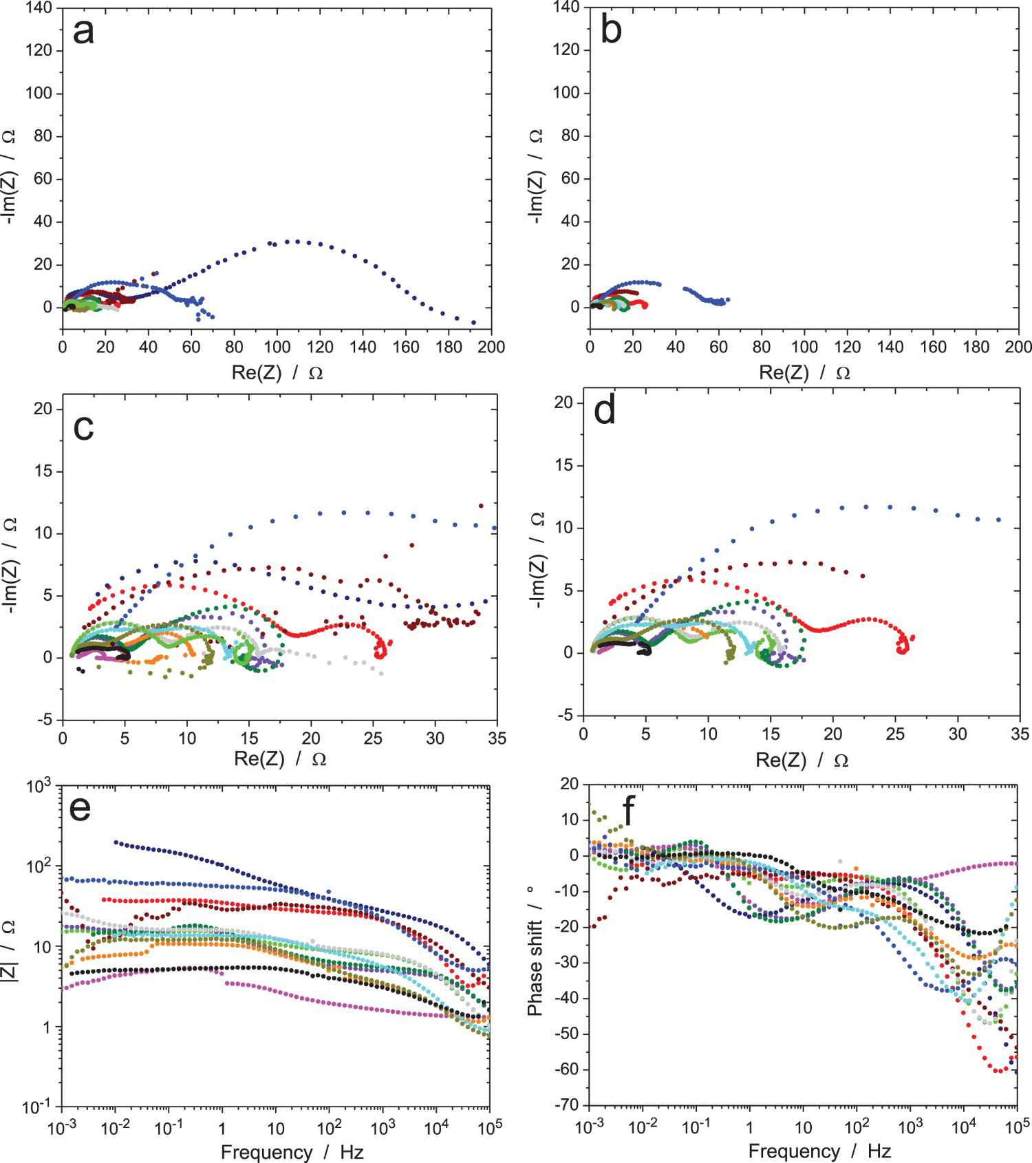
EIS data for the Zr/Na₂SO₄ system (RR3, measurement A: immersion time 6 h, ΔV = 20 mV_rms): (a) Nyquist and (b) Bode diagrams of raw data (10 participants).

Figure 11

EIS data for the Zr/Na₂SO₄ system (RR3, measurement B: immersion time 24 h, ΔV = 20 mV_rms): (a and c) Nyquist and (b and d) Bode diagrams of (a and b) raw data and (c and d) data validated by indirect integration with an error lower than 3% (10 participants).

Figure 12

EIS data for the Zr/Na₂SO₄ system (RR3, measurement C: immersion time 120 h, ΔV = 20 mV_rms): (a) Nyquist diagram; (b) Bode plots of raw data (10 participants).

Figure 13

EIS data for the Zr/Na₂SO₄ system (RR3, measurement D: immersion time 168 h, ΔV = 20 mV_rms): (a) Nyquist diagram; (b) Bode plots of raw data (10 participants).

Figure 14

EIS data for the Zr/Na₂SO₄ system (RR3, measurement E: after measurement D, ΔV = 2 mV_rms): (a) Nyquist diagram; (b) Bode plots of raw data (10 participants).

Figure 15

EIS data for the Zr/Na₂SO₄ system (RR3, measurement F: after measurement E and 15 min at OCP, ΔV = 5 mV_rms): (a) Nyquist diagram; (b) Bode plots of raw data (10 participants).

Figure 16

EIS data for the Zr/Na₂SO₄ system (RR3, measurement G: after measurement F and 15 min at OCP, ΔV = 50 mV_rms): (a) Nyquist diagram; (b) Bode plots of raw data (10 participants).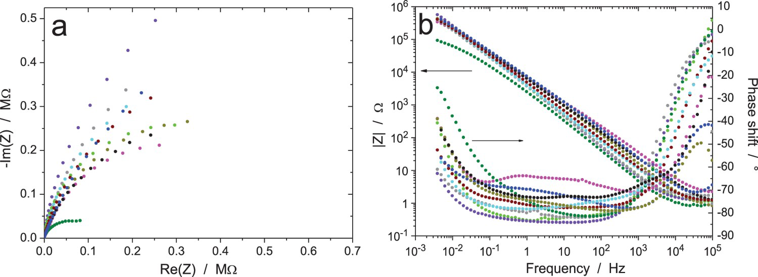

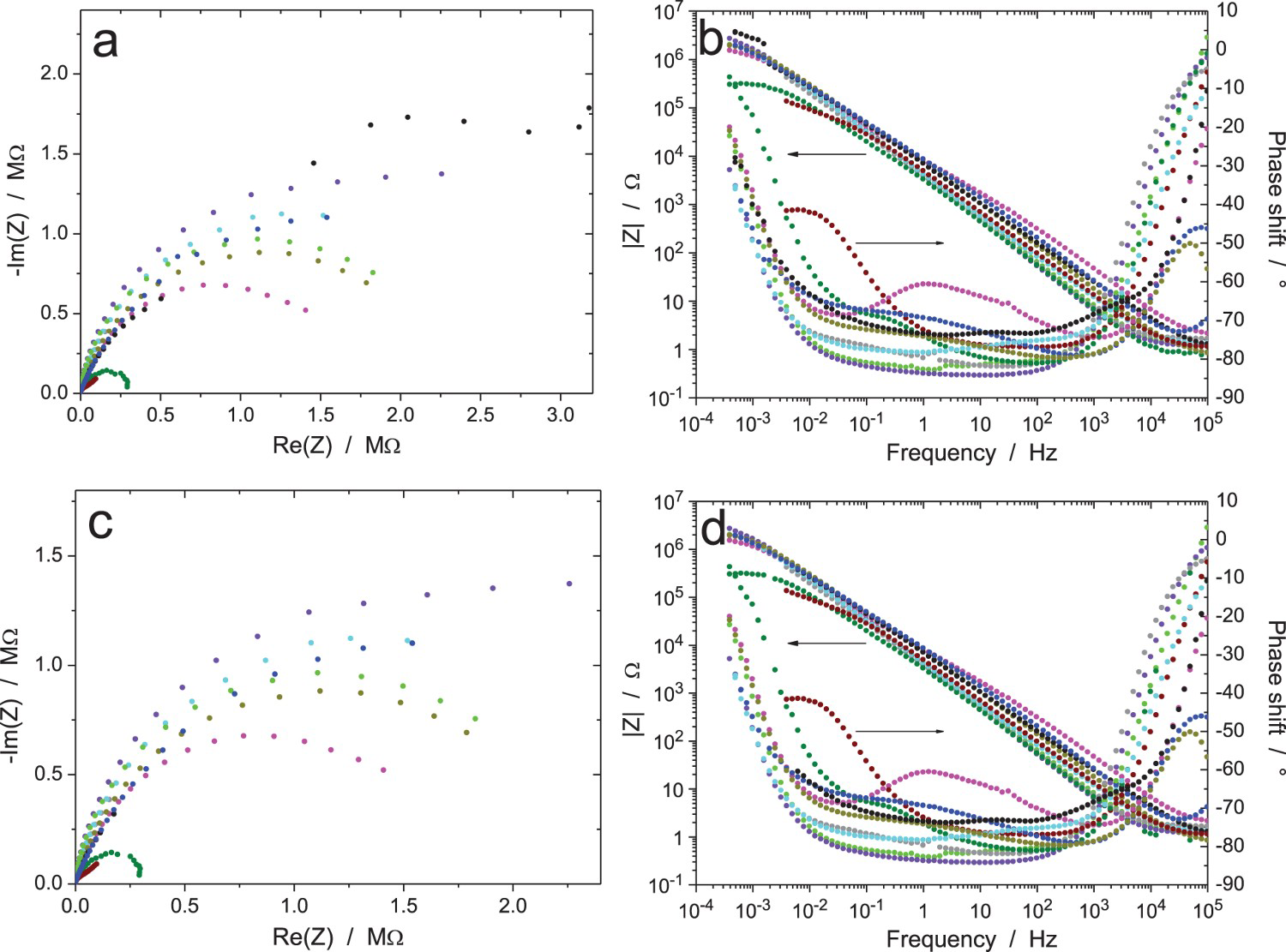
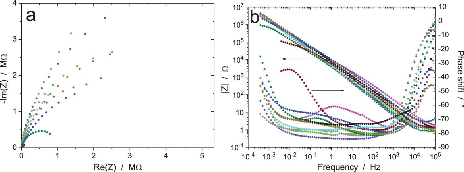
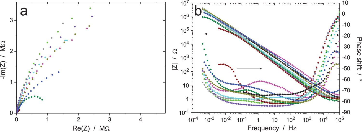
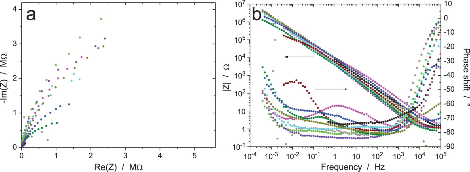
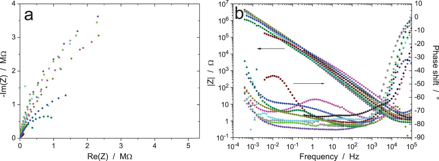
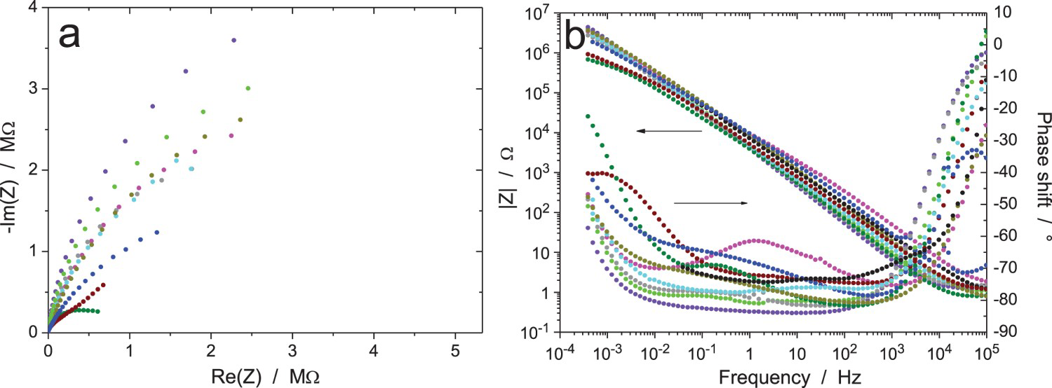
Figure 10 shows the results after 6 h of exposure with an amplitude of 20 mV_rms (measurement A) for the excitation signal. Results are free of noise and all show the same behaviour, except one system (olive curve) with a lower impedance modulus at low frequency than the others. Small differences are present in the modulus, with a factor of three between the minimum and maximum values at 1 Hz and a factor of six at 10 kHz, and some discrepancies are also exhibited in the measured phase shift. This is most probably caused by small differences in the thickness of the oxidation layer on the Zr wire, possibly due to small variations in the specimen surface preparation, or to different waiting times between surface grinding and exposure to the test solution, or also to environmental parameters such as temperature and humidity. Even if the Zr wire was provided by the same manufacturer and the surface preparation procedure was indicated in the testing procedure, it was impossible, as usual, to have perfectly identical experimental conditions in different laboratories participating to an RR exercise. All measured impedances have a standard shape, only the blue impedance modulus curve increasing with frequency above 50 kHz shows an unusual shape, possibly due to a too-resistive reference electrode. All raw data in Figure 10 have been validated by indirect integration, including the modulus curve giving a phase shift close to -40° at 100 kHz (blue curve), which was not validated by direct integration.

Figures 11–13 show the results after 24, 120 and 168 h of exposure, still with an amplitude of the excitation signal of 20 mV_rms (measurements B, C and D, respectively). As expected, the impedance modulus increased with time at low frequency, because of the thickening of the oxide layer, and reached values above 1 MΩ. Curiously, another system showed a much lower modulus at low frequency (about 1 kΩ in Figure 11, burgundy colour) showed a different behaviour, probably because the oxide film did not cover the electrode surface perfectly so that an electrochemical reaction could occur on the unprotected surface area. A discontinuity in the impedance modulus at 1.6 mHz can also be noted for one test (black colour in Figure 11b); it was probably due to an automatic change of the current-measuring resistor in the potentiostat. As shown in Figure 11(c,d), all the raw data in Figure 11(a,b) have been validated by indirect integration, with the exception of the black impedance curve at low frequency. For better clarity in the Nyquist diagrams, the low-frequency part of the black impedance curve has not been plotted in the following figures.

The results of the impedance measurements after 168 h of exposure are shown in Figures 14–16 for an increasing value of the amplitude of the perturbation signal of 2, 5 and 50 mV_rms (measurement E, F, G, respectively). All raw data have been validated by indirect integration with the obvious exception of a few ‘wild’ points, especially in Figures 14 and 15 because of the low amplitude of the excitation signal. Roughly speaking, all results are similar to the previous ones with a clear improvement of the measurement accuracy when increasing the amplitude of the excitation signal. However, it is not possible to conclude on the quality of the result when comparing the data provided by the 10 participants on the same plot. Therefore, the impedance data measured by two different participants were plotted in Figure 17 to show the results obtained with two different equipment. In both Nyquist diagrams, the magnitude of the impedance clearly increases during the first 120 h of immersion (measurements A, B and C) indicating the thickening of the oxide layer, but later this phenomenon seems to reach a maximum since the curve for measurement D is slightly below that of measurement C in Figure 17(b), even if this case is not the most representative among the 10 data sets. Concerning the influence of the amplitude of the excitation signal on the impedance data, it can be seen in Figure 17 that, for both participants, the effect was not significant when using an amplitude ΔV _rms lower than 20 mV. However, when using an amplitude of 50 mV_rms (measurement G), the conclusion is not straightforward since in Figure 17(a) curve G is below curves E and F, while in Figure 17(b), curves B, E and F are very close to each other. Both cases were encountered by the other participants. It should also be noted that the accuracy of the impedance diagram measured with an excitation amplitude of 2 mV_rms was good for some equipment, as shown in Figure 17, while the diagram was very noisy for some other equipment.

Figure 17

EIS raw data for the Zr/Na₂SO₄ system (RR3): influence of the immersion time and amplitude of the voltage excitation for two different participants (a and b) using two different equipment.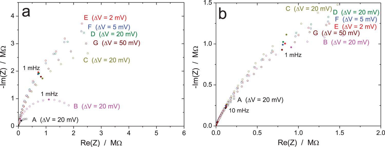

In conclusion, all devices gave good results for the Zr/Na₂SO₄ system even when the impedance exceeded 1 MΩ. Only the combination of the smallest amplitude and maximum impedance (∼3 MΩ) resulted in noisy data for some devices. Most probably, this is related to the settings of the instrument and/or background noise in the test laboratory.

The scatter in the impedance data observed in the RR exercises involving electrochemical systems may be surprising for experienced EIS users. However, this is a common feature of RR exercises to find different results with well-functioning measurement instruments. In this exercise, all EIS measuring devices performed well, as shown in RR1. The scatter can be explained by different factors. First, it is well known that the reproducibility of corrosion experiments is often poor because it is impossible to have exactly the same material and experimental conditions in the different laboratories, even if the electrodes were prepared in the same way and sent to all participants who did their best to follow as much as possible the experimental recommendations given in the testing procedure. This is an original output of this work, which does not at all put into question the reliability of the EIS technique. Second, an RR test is not a complete investigation of a given (electrochemical) system. Its role is to study the reproducibility of EIS measurements performed by different laboratories and instruments by comparing the results sent by all participants. The measurements were not repeated by each participant in his laboratory, it is then not possible to assess the reproducibility of EIS measurements performed in a given laboratory. In a sense, the EIS data on a given system sent by each participant are like the data obtained the first time by a common user who will then perform again his experiment to test its reproducibility and understand the possible impact of each parameter (size and position of each electrode, temperature, etc.) of his electrochemical cell on the measured impedance. This is what is expected from the researchers publishing EIS investigations, not from an RR exercise.

Conclusions

Three RR exercises were carried out on EIS measurements with (1) a dummy cell, (2) a Cu/CuSO₄ system and (3) a Zr/Na₂SO₄ system to assess to which extent the equipment and laboratory lead to comparable results. The originality of the current work is the presentation, for the first time to the best of our knowledge, of an RR test involving a very large number of laboratories [19]. The first trial with a dummy cell of impedance magnitude ranging from 100 Ω to 5 MΩ showed very good results, indicating that all actual commercially available instruments for EIS measurements performed well in the frequency range from 0.1 mHz to 100 kHz. The second trial with the Cu/CuSO₄ system showed that clear differences in results between the different participants were obtained and that there was a pronounced influence of the amplitude of the excitation signal, which had to be set well below the common value of 10 mV_rms. The main cause for the different results is the difficulty of measuring the impedance of a ‘non-polarisable’ system like a reference electrode. It could be concluded that the Cu/CuSO₄ system was not adequate for performing an RR test, but it can also be considered that the exercise better demonstrates the care that needs to be taken when measuring the impedance of an electrochemical system, and the scatter in the results is more informative for a common EIS user than identical results obtained by the participants on an easy system. The third trial with a system whose impedance exceeded 1 MΩ showed good reproducibility in the shape and time evolution of the impedance diagrams for the different participants, with an inevitable variation of the impedance magnitude as for any electrochemical system implemented in different laboratories.

Validation of the measured impedance data to check their compliance to Kramers–Kronig relations was performed, which allowed the elimination of errant points or signal drift effects. The fact that most impedance diagrams were successfully validated indicates that the dispersion in the impedance results, obtained for both tested electrochemical systems, the largest difference being for the Cu/CuSO₄ system, comes from variations in the experimental conditions in the different laboratories (wire surface preparation, waiting times in solution, etc.). This reveals that the experimental parameters should have been more thoroughly defined in the RR testing procedure.

The general conclusion is that EIS is an excellent technique for investigating the kinetics of electrochemical systems, but that the measurements have to be planned and performed very carefully. This is actually true for all experimental techniques and should always be kept in mind. Great care has to be taken, e.g. repeating measurements to check reproducibility, as the RR test shows that to a certain extent, intrinsic scatter is always present. Training with dummy cells that mimic the measured electrochemical impedance is also recommended in order to validate EIS measurements.

Footnotes

Acknowledgements

The support from the members of the European Cooperative Group on Corrosion Monitoring of Nuclear Materials (ECG-COMON, ) is gratefully acknowledged. Special thanks are expressed to Christian Bataillon (CEA Saclay, France), Zsolt Kerner (MTA EK, Hungary), Bo Rosborg (KTH, Sweden), Peter Schrems (IPS Elektroniklabor, Germany) and Max Yaffe (Gamry Instruments, USA) for their participation to the RR exercises.

Disclosure statement

No potential conflict of interest was reported by the authors.

Appendix

References

Bosch

R-W

Cottis

Csecs

. Reliability of electrochemical noise measurements: results of round-robin testing on electrochemical noise. Electrochim Acta. 2014; 120: 379–389.

Huet

Ritter

Electrochemical noise measurements with dummy cells: Evaluation of a round-robin test series. Corrosion. 2018; 74: 1457–1465.

Macdonald

McKubre

MCH.

Electrochemical impedance techniques in corrosion science. In: Mansfeld

Bertocci

, editors. Electrochemical corrosion testing, STP 727. West Conshohocken (PA): American Society for Testing and Materials; 1981. p. 110–149.

Scully Jr Silverman

Kendig

(Eds). Electrochemical impedance: analysis and interpretation, STP 1188. West Conshohocken (PA): American Society for Testing and Materials; 1993.

Gabrielli

Use and applications of electrochemical impedance techniques. Technical Report 24, Solartron Analytical; 1997 [cited 2020 September 22]. Available from: https://www.ameteksi.com/-/media/ameteksi/download_links/documentations/library/solartonanalytical/electrochemistry/technical-report-24-gabrielli-applications-of-eis.pdf.

Macdonald

JR.

Impedance spectroscopy emphasizing solid materials and systems. New York: Wiley; 1987.

Cottis

Turgoose

Electrochemical impedance and noise. In: Syrett

, editor. Corrosion testing made easy. Houston (TX): NACE International; 1999.

Stoynov

Savova-Stoynov

BS.

Impedance study of non-stationary systems: four-dimensional analysis. J Electroanal Chem Interfacial Electrochem. 1985; 183: 133–144.

Breugelmans

Lataire

Muselle

. Odd random phase multisine electrochemical impedance spectroscopy to quantify a non-stationary behaviour: theory and validation by calculating an instantaneous impedance value. Electrochim Acta. 2012; 76: 375–382.

10.

Koster

Battistel

. Dynamic impedance spectroscopy using dynamic multi-frequency analysis: a theoretical and experimental investigation. Electrochim Acta. 2017; 246: 553–563.

11.

Macák

Novotný

Sajdl

. In-situ electrochemical impedance measurements of corroding stainless steel in high subcritical and supercritical water. Corros Sci. 2019; 150: 9–16.

12.

de Araújo Figueiredo

Bosch

Vankeerberghen

Electrochemical investigation of oxide films formed on nickel alloys 182, 600 and 52 in high temperature water. Electrochim Acta. 2011; 56: 7871–7879.

13.

Bosch

Vankeerberghen

In-pile electrochemical tests of stainless steel under PWR conditions: interpretation of electrochemical impedance spectroscopy data. Electrochim Acta. 2007; 52: 7538–7544.

14.

Lasia

Electrochemical impedance spectroscopy and its applications. New York (NY): Springer; 2014.

15.

Orazem

Tribollet

Electrochemical impedance spectroscopy. 2nd ed. New York (NY): Wiley; 2017.

16.

ISO 16208. Corrosion of metals and alloys – test method for corrosion of materials by electrochemical impedance measurements. Geneva: International Organization for Standardization; 2014.

17.

ISO 16773. Electrochemical impedance spectroscopy (EIS) on coated and uncoated metallic specimens. Geneva: International Organization for Standardization; 2016.

18.

STM G106-89. Standard practice for verification of algorithm and equipment for electrochemical impedance measurements. West Conshohocken (PA): American Society for Testing and Materials; 2015.

19.

Vogelsang

Bakalli

Electrochemical impedance spectroscopy measurements on organic coatings according to the standard ISO 16773-2: evaluation of a round-robin test and introduction to ISO technical report on measurement artefacts. 11th International Symposium on Electrochemical Impedance Spectroscopy 2019; Lège-Cap-Ferret, France ; 2019 June 2-7.

20.

Agarwal

Orazem

Garcia-Rubio

LH.

Application of measurement models to impedance spectroscopy: III. Evaluation of consistency with the Kramers-Kronig relations. J Electrochem Soc. 1995; 142: 4159–4168.

21.

Boukamp

BA.

A linear Kronig-Kramers transform test for immittance data validation. J Electrochem Soc. 1995; 142: 1885–1894.

22.

Schönleber

Klotz

Ivers-Tiffée

A method for improving the robustness of linear Kramers-Kronig validity tests. Electrochim Acta. 2014; 131: 20–27.

23.

Boukamp

BA.

Kramers-Kronig data validation programme equivcrt, University of Twente [cited 2020 September 22]. Available from: https://www.utwente.nl/en/tnw/ims/publications/downloads.

24.

Boukamp

BA.

Electrochemical impedance spectroscopy in solid state ionics: recent advances. Solid State Ionics. 2004; 169: 65–73.

25.

Gabrielli

Keddam

Takenouti

Kramers-Kronig transformation in relation to the interface regulating device. In: Scully Jr Silverman

Kendig

, editors. Electrochemical impedance: analysis and Interpretation, ASTM STP 1188. West Conshohocken (PA): American Society for Testing and Materials; 1993. p. 140–153.

26.

Ives

DJG

Janz

GJ.

Referenced electrodes: Theory and practice. London: Academic Press; 1961.

27.

Stoynov

Savova

Instrumental error in impedance measurements of non-steady-state systems. J Electroanal Chem Interfacial Electrochem. 1980; 112: 157–161.

28.

Rakotomavo

Etude par mesure d'impédance de la nature des polarisations à l'électrode positive d'un accumulateur au plomb [PhD Thesis]. Paris, France: University Paris 7; 1983.

Results of an international round-robin exercise on electrochemical impedance spectroscopy

Abstract

ABSTRACT

Keywords

Introduction

Experimental

Part 1: Dummy cell

Parts 2 and 3: Electrochemical systems

Reporting and analysis

Results and discussion

Part 1: Dummy cell

Part 2: Cu/CuSO4 electrochemical system

Part 3: Zr/Na2SO4 electrochemical system

Conclusions

Footnotes

Acknowledgements

Disclosure statement

Appendix

References

Part 2: Cu/CuSO₄ electrochemical system

Part 3: Zr/Na₂SO₄ electrochemical system