Prediction of surf-zone and open-ocean airborne sea-salt spatial distribution via computational fluid dynamics and statistical method

Abstract

The atmospheric corrosion of steel is a critical design and maintenance issue for structures such as electric transmission towers and bridges, which are generally widely dispersed. As airborne sea-salt particles are a major corrosion factor, the long-term cumulative spatial distributions of sea salt deposited on the structure surfaces are needed. In this study, we predict the long-term cumulative spatial distribution of sea-salt particles originating from the surf zone and from the open ocean, combining a computational fluid dynamics simulation and a statistical procedure. A new prediction method is introduced for sea-salt particle concentration originating from the surf zone and is validated based on comparisons with observed data. The predicted results indicate that surf-zone-originating particles increase remarkably the amount of airborne sea-salt particles near the coastline and can travel more than 5 km inland.

Keywords

Atmospheric corrosion steel structure sea-salt particle numerical simulation statistical method

Introduction

The atmospheric corrosion of steel is a major problem as it requires maintenance of the outdoor structures such as electric transmission towers and bridges. The steels used in these structures, typically hot-dip galvanised and/or coated with anticorrosion paints, suffer from corrosion during their long-term operation; this is particularly true for structures located near coastal areas. Thus, efficient planning of maintenance activities and effective design and materials selection to combat the corrosion of such structures are a worldwide concern (e.g. [1,2]). A major factor causing the corrosion is long-term exposure to airborne sea-salt particles (e.g. [3]). While the amount of airborne sea-salt particles decays exponentially with increasing distance from the coast, they vary markedly according to the different offshore winds (e.g. [4]). There is also the local variation according to the topography and ground roughness to consider (e.g. [5,6]).

Most sea-salt particles are generated from the breaking of waves in the open ocean (OO) by wind action. In the 1950s and 1960s, pioneering studies on the number and weight of sea-salt particles generated at sea were conducted, based on observations and experiments (e.g. [7,8]). These works were followed by many studies on production flux models for sea-salt particles; the outcome of these models was treated as source terms in numerical simulations of sea-salt particle transport (for details, see [9 11]). However, sea-salt particles are also generated from waves breaking in shallow sea areas near the coastline because of water depth limitations; these are surf-zone-originating (SZ) particles. Thus, models for predicting the SZ particle production fluxes, expressed as a function of particle diameter occasionally with the wind velocity or the energy dissipation of the wave as a variable, have also been proposed [12 14].

Numerical simulations are an effective means of evaluating the amount of airborne sea-salt particles, and the above-mentioned models concerning sea-salt particle generation have been used in previous simulations: for instance, de Leeuw et al. [12] applied their own SZ model to a simple transport simulation. It indicated that the SZ particles contribute significantly to particle concentration at distances of at least 25 km from the coastline. Tedeschi et al. [15] also performed numerical simulations with OO and SZ models, finding that the SZ particles contribute significantly during high wind velocities and high wave events. Regardless, there are still very few studies on SZ particles, leading to insufficient knowledge for the spatial distribution of the long-term accumulated SZ particles.

Suto et al. [16] proposed a method combining a computational fluid dynamics (CFD) simulation and a statistical procedure to estimate the spatial distribution of long-term accumulated sea-salt particles. This method allows the prediction of the spatial distributions of long-term cumulative sea-salt mass, while considering the effects of offshore wind velocity, topography and ground roughness. When only the OO particle generation process was considered, the predicted values correlated significantly with observed values. However, some values tend to be underestimated near the coast, suggesting that consideration of the SZ particles may improve the prediction accuracy. In this study, we introduce a novel method for estimating the SZ particle concentration while also using the Suto et al. [16] method to predict the spatial distribution of sea-salt particles originating from both the OO and SZ. We also discuss the properties of the OO and SZ particles transported inland.

The remainder of this paper is organised as follows. In the ‘Numerical method’ section, we show the equations used to estimate the concentration of OO particles and propose a novel method for estimating the concentration of SZ particles. An outline of the CFD simulation and the statistical procedure is also provided. In the ‘Prediction of airborne sea salt originating from open ocean and surf zone’ section, the amounts of airborne sea salt originating from the OO and SZ are predicted; the accuracy is evaluated by comparison with existing observation data. The ‘Characteristics of ocean- and surf-originating particles transported inland’ section discusses the characteristics of the particles transported inland.

Numerical method

CFD simulation

The basic equations used in the CFD simulation are the continuity, Navier–Stokes and sea-salt concentration transport equations described in boundary-fitted coordinates [16]. The standard k–ϵ model was applied as a turbulence model, and the turbulent Schmidt number was set to 1.0. A third-order upwind finite difference was applied to the advection terms and a second-order central finite difference was applied to all other terms for spatial discretisation. The Crank–Nicolson method was applied for time marching.

The inlet boundary was set on the sea, where a wind velocity distribution based on the logarithmic law was given. An equation for the sea-salt concentration in terms of the wind velocity and the sea fetch, the details of which are described in the ‘Concentration of particles reaching the coastline’ section, was applied. At the ground boundary, the wind velocity was calculated from a logarithmic law considering the ground roughness, and sea-salt concentration was deduced from the deposition model of Lewellen and Sheng [17].

Concentration of particles reaching the coastline

In the CFD simulation, the inflow boundary was set on the sea, as described above. The following equations, based on the Toba [8] model, were adopted for the distribution of the OO particles [16]:

(1) (2)

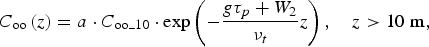
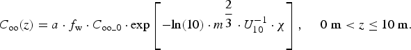
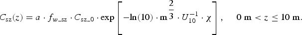
Here, the subscript ‘ ’, ‘10’ and ‘0’ represent the OO, and the heights of 10 and 0 m, respectively, while is the concentration reduction factor as a function of , and ; the sea-salt concentration; the sea-salt particle diameter; the fetch; the wind velocity factor; the gravity acceleration; the sea-salt nucleus mass; the wind velocity; the velocity of descending air (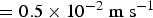); z the height; the air kinetic viscosity; the air density; the sea-salt particle density; and the velocity relaxation time 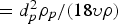; the coefficient ().

Additionally, the following equations showing the concentration distribution of SZ particles are proposed in this work, based on Equations (1) and (2) (3) (4)

Here, the subscript ‘ ’ represents the SZ, while the following definitions apply: is the concentration reduction factor as a function of , and ; is the SZ width; and the wind velocity factor for the concentration of SZ particles. Note that Equations (3) and (4) assume a similarity between two processes: the concentration of OO particles increasing with the fetch and the second of the concentration of SZ particles increasing with the SZ width. This assumption is based on the premise that the vertical distributions of the particle concentration at a wind velocity can be normalised by the concentration on the sea surface, which is consistent with the Toba [8] model and the mass transport similarity in boundary-layer flows (e.g. [18]). Moreover, as and are assumed to indicate the respective particle concentrations reaching the coastline, it is desirable for them to hold the distribution of Equations (1)–(4) between the inlet boundary on the sea and the coastline, unless those particles are not affected by the topography. To realise this, a source term suppressing the vertical diffusion of the sea-salt concentration on the sea only was added to the sea-salt concentration transport equation [19]. Note that in the methods for feeding SZ particles as a flux from the sea surface adopted in previous numerical simulations (e.g. [15]), the particle concentration distribution at the coastline may be strongly affected by the numerical parameters (such as the grid resolution); however, our proposed method is unaffected by this issue.

Concerning the parameters of the above-mentioned particle concentration distribution, the value was identified from the land-use data described in the ‘Numerical conditions’ section [16]. The value was set to 200 or 50 m (representative values), as it is typically a few hundred metres. The parameters and were set to . This setting corresponds to the observation by de Leeuw et al. [12] that the concentrations of OO and SZ particles differ by more than 10 times (the correspondence with existing models is described in the ‘Numerical results for concentration of particles reaching coastline’ section). The value was determined using a numerical simulation code reproducing the generation, advection, diffusion and sedimentation processes of sea-salt particles [16,20].

Statistical procedure

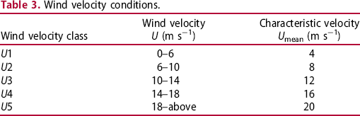
To efficiently estimate the spatial distributions of the cumulative amount of airborne sea salt, the following procedures were adopted [16]: (1) the wind directions, wind velocities and particle sizes were divided into classes, and the wind and sea-salt particle transport were numerically simulated for each class, (2) the occurrence frequencies of the wind direction and velocity at arbitrary locations were estimated using statistical wind data obtained at ∼10 km offshore and (3) the cumulative or period-averaged amount of airborne sea salt were calculated by adding the CFD results for all wind direction, wind velocity and particle size classes, weighted with their occurrence frequencies.

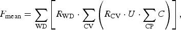
In procedure (3), the period-averaged amount of airborne sea salt (sea-salt advection flux) was calculated from the following equation: (5) where is the particle size class, the wind velocity class, the wind direction and the occurrence frequency of . As the amount of airborne sea salt is approximately proportional to the amount of deposited sea salt [21] within a region where the degree of rain washing from structure surfaces and the deposition efficiency are almost identical, the airborne sea salt was used as an indicator for comparison with the deposited sea-salt observation data discussed below.

Prediction of airborne sea salt originating from open ocean and surf zone

Numerical conditions

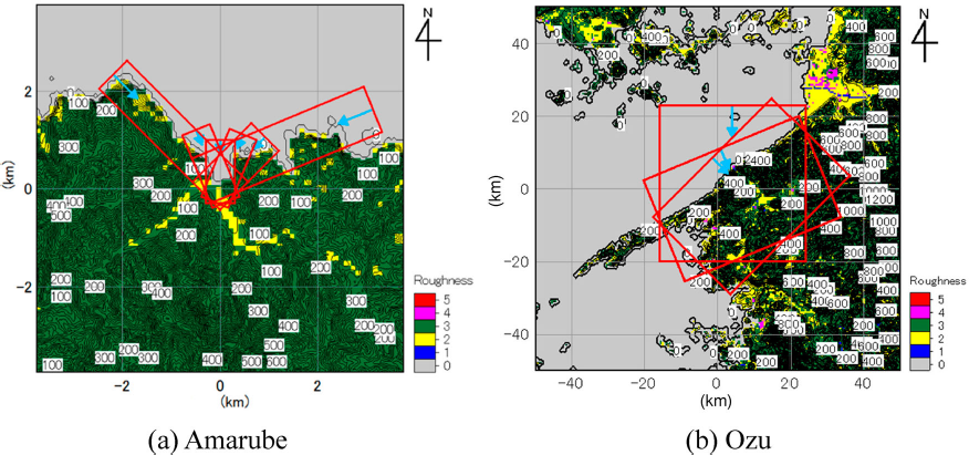
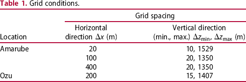
To evaluate the airborne sea-salt particles in a coastal area and inland, regions were selected where previous observation data were available for comparison with the predicted values. Specifically, the Amarube region (Hyogo Prefecture, Japan) was selected for evaluation of the sea salt in a coastal area, while the Ozu region (Ehime Prefecture, Japan) was selected for evaluation of sea salt transported inland.

The computational domains for each wind direction are indicated by the rectangular frames in Figure 1. The selected directions correspond to sea winds with a high occurrence frequency and high mean wind velocity. Note that the domain sizes in the Amarube and Ozu regions differ by approximately one order of magnitude. The grid conditions are listed in Table 1. The grid spacing in the vertical direction (minimum value) was set in the range of 10-20 m near the ground, to accurately capture the vertical distribution of the particle concentration. The grid spacing in the horizontal direction was set to one of four values in the range of 20-400 m, referring to the empirical criterion of 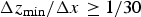for numerical stability. Three different grid systems were applied to evaluate the resolution effect. The was set to one of the two values (200 and 50 m) to evaluate its sensitivity, mentioned above.

Figure 1

Computational domains.

Table 1

Grid conditions.

Location	Grid spacing
Horizontal direction (m)	Vertical direction (min., max.) , (m)
Amarube	20	10, 1529
	100	20, 1350
	400	20, 1350
Ozu	200	15, 1407

To set the topography and ground roughness, a 10 m mesh digital elevation model from the Geospatial Information Authority of Japan and 100 m mesh land-use data from the Ministry of Land, Infrastructure, Transport and Tourism, were used, respectively. The high-resolution and long-term meteorological dataset CRIEPI-RCM-Era2 [22], which reproduces the weather for the past 53 years (1957-2010), was used as the statistical data source for the offshore wind. The particle size and wind velocity were classified into three and five classes, respectively, as detailed in Tables 2 and 3 [16].

Table 2

Sea-salt particle conditions.

Particle size class	Logarithm of mass of salt content −log m (kg)	Mean mass of salt content m (kg)	Number concentration (1/m³) (OO, wind velocity 4.4 m s⁻¹)	Particle diameter d_p (m) (relative humidity 80%)
P1	14.5-13.0	1.75 × 10⁻¹⁴	3.00 × 10⁵	4.94 × 10⁻⁶
P2	13.0-12.0	3.53 × 10⁻¹³	4.84 × 10⁴	1.34 × 10⁻⁵
P3	12.0-11.0	4.01 × 10⁻¹²	6.88 × 10⁴	3.02 × 10⁻⁵

Table 3

Wind velocity conditions.

Wind velocity class	Wind velocity U (m s⁻¹)	Characteristic velocity U _mean (m s⁻¹)
U1	0-6	4
U2	6-10	8
U3	10-14	12
U4	14-18	16
U5	18–above	20

Observation data for accuracy evaluation

In this section, we outline the existing observation data used to evaluate the prediction accuracy in the ‘Accuracy evaluation’ section.

For the Amarube region, the observation data for the deposited sea salt (on painted steel plates and dry gauze) and the weight loss of unpainted steel plates (SS400) due to corrosion were used; the plates and gauze were vertically oriented facing the sea at multiple points of the original Amarube trestle bridge, located near an intricate coastline [23]. The detailed location and height are mentioned in the ‘Numerical results for spatial distribution of airborne sea-salt particles’ section. Concerning the data on the sea-salt deposition on the steel plates, the plates were washed using pure water to remove the deposited substance from the surface after exposure for 1 month. The chloride ion content of the obtained water was measured and converted to equivalent salt content. The data regarding the sea-salt deposition on dry gauze placed under rain protection were obtained on considering the JIS Z 2382 standard. The salt content was measured using the same procedure as for the steel plates. The average values of monthly data obtained over ∼5 years were used to compare with the predicted results. Regarding the weight loss data, after an exposure of ∼5 years, the corrosion products were removed using a sulphuric-acid aqueous solution; then, the variation in each plate weight was measured.

For the Ozu region, the observation data for the sea salt deposited on insulators installed on transmission towers were used [16]. The observation points and their point numbers are shown in Figure 2. The insulator ground height was ∼5-20 m. As the measurement method, a manual washing method (e.g. [24]) was used, where all the ground-facing surfaces of the contaminated insulators were washed with pure water. The equivalent salt content was then calculated from the resistivity of the obtained water. The average value of monthly data over ∼5 years was compared with the predicted results.

Figure 2

Observation data locations in Ozu.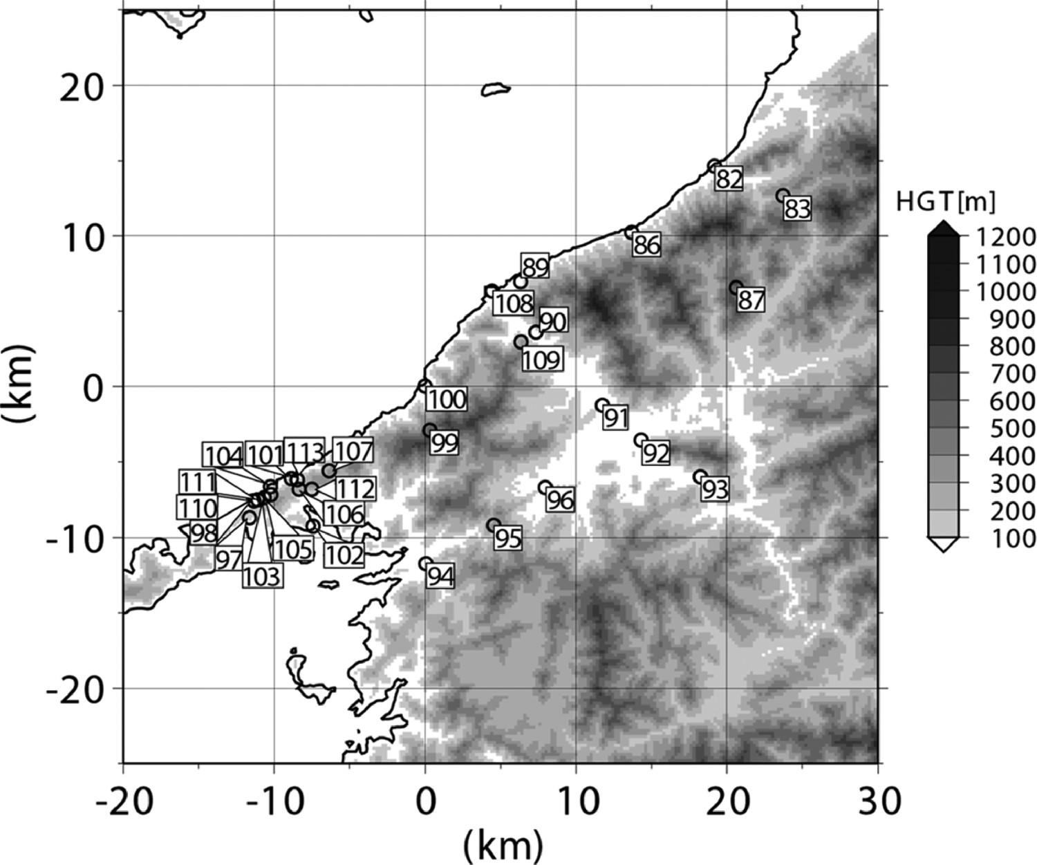

Numerical results for concentration of particles reaching coastline

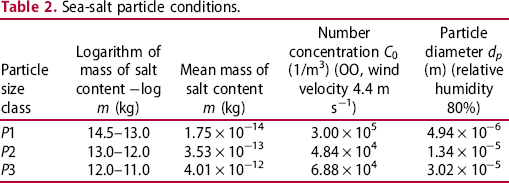
Here, we pay attention to the concentrations of OO and SZ particles calculated using Equations (1)–(4) and their relationship with an existing representative model for the particle production on the sea surface. As an example, Figure 3 shows the concentration distributions of OO particles and both OO and SZ (OO + SZ) particles, which reach the coastline when . The symbols P1–P3 correspond to particle diameters of 4.9, 13.4 and 30.2 µm, respectively (Table 2). The SZ particle effects obviously appear in the range of 0-100 m. Figure 4 shows the production flux of the number of sea-salt particles , determined from the production flux model of Monahan et al. [25], and the number concentration on the sea surface , obtained from Equations (1) to (4) and the parameters set in the ‘Concentration of particles reaching the coastline’ section; these characteristics are shown for each particle size. Note that in the figure represents the concentration on the sea surface. represents the particle radius at 80% relative humidity. In the existing model, the dependence of the whitecap fraction on the wind velocity was considered for the flux on OO , whereas was set to unity for the flux on SZ [12]. The Toba [8] model, which is the basis for Equations (1)–(4), focuses on relatively large particles possibly closely related to salt damage and spans a particle size range larger than that of Monahan et al. [25]. Note that it is inappropriate to directly compare the concentration to the production flux, as the relationship between them is determined by a balance of elementary processes such as the production, gravitational sedimentation, turbulent diffusion and particle deposition, and the balance depends on the particle size and wind velocity (e.g. [26]). However, we can confirm that the variations in the flux and concentration for particles with different origins and sizes are similar.

Figure 3

Vertical distributions of sea-salt concentration at coastline (, P1: 4.9 µm, P2: 13.4 µm, P3: 30.2 µm).

Figure 4

Variations in particle flux and concentration on sea surface with particle size ().

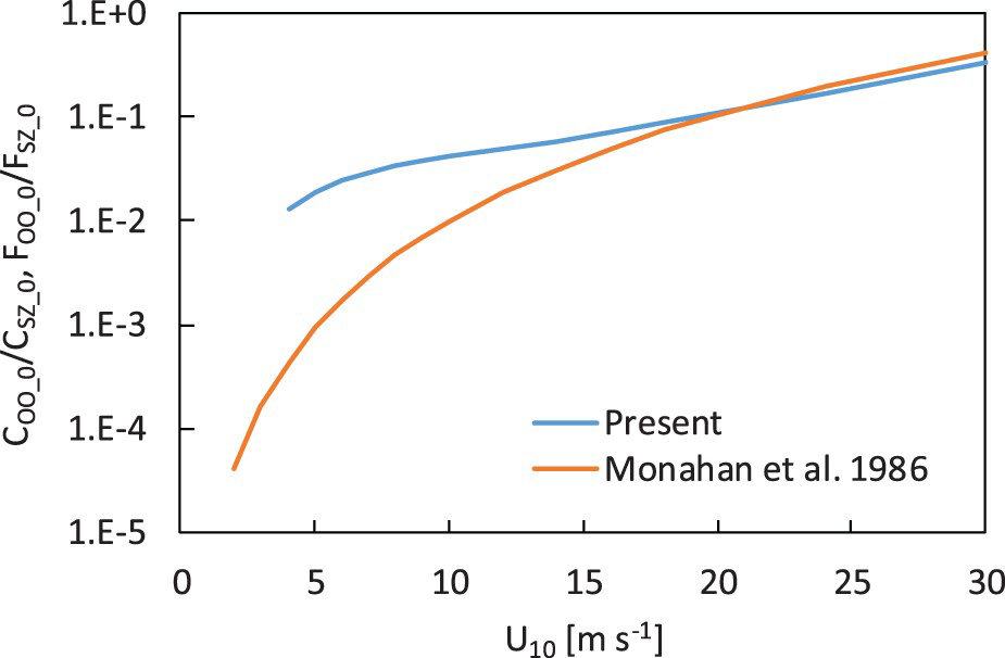
Figure 5 shows the ratios of the OO- to SZ-originating sea-salt concentrations and production fluxes according to the wind velocity. The Monahan et al. [25] line corresponds to the whitecap fraction described above. Note that the proposed here is independent of the wind velocity ( is constant), as in Clarke et al. [13]. This causes the concentration ratio to tend asymptotically towards one with wind velocity, similar to the Monahan et al. [25] flux ratio. Note also that there is a large dispersion of one or two orders of magnitude between the flux values obtained from many previous models and observations (e.g. [11]). Although the ratios in our model, based on Toba [8], are separated from those of the Monahan et al. [25] model in a low-wind velocity range, the causes are not only the uncertainties of the existing models, but also the dependence of the above-mentioned relationship between the production flux and concentration on the wind velocity.

Figure 5

Ratios of OO particle flux and concentration to those of SZ particles.

Numerical results for spatial distribution of airborne sea-salt particles

The distributions of the annual mean amounts of airborne sea salt for the OO only and the OO + SZ in Amarube are shown in Figures 6 and 7, respectively. Points 2P–10P in the figures indicate the positions of the bridge piers where the observation data were acquired. The results indicate that the airborne sea-salt decay with distance from the coastline is non-uniform, reflecting the effects of the intricate coastline and topographical undulation. Note that the values for OO + SZ in Figure 7 are multiplied by 0.5 to magnify the variation. When the SZ particles are considered, the absolute amount of airborne sea salt increases as a whole, and that near the ground surface along the coastline increases markedly.

Figure 6

Annual mean amount of airborne sea salt (Amarube, OO, , ).

Figure 7

Annual mean amount of airborne sea salt (Amarube, OO + SZ, , ).

Figure 8 shows the vertical distributions of the amount of airborne sea salt for the OO only and the OO + SZ for each wind direction at point 4P in Amarube. The values for the SZ sea salt are larger than those of the OO sea salt near the surface and decrease with increasing height, corresponding to Figure 3. However, there is a large decrease in the values in the vicinity of the ground surface in accordance with low near-surface wind velocities as well as particle deposition on the ground. This is because the amount of airborne sea salt is dependent on both the wind velocity and the concentration (Equation (5)). Moreover, the values remarkably vary with the wind direction, indicating that the distance from the coastline, offshore wind velocity and windward topography, which all vary with the wind direction, affect the amount of airborne sea salt.

Figure 8

Amount of airborne sea salt in each wind direction (Amarube, , , location 4P).

The distributions of the annual mean amount of airborne sea salt for the OO only and the OO + SZ in Ozu are shown in Figure 9. The results indicate an attenuation according to the distance from the coastline and local variations based on topography. The results are similar to those of Amarube in that the absolute amount of airborne sea salt increases overall and the amount near the coastline increases in particular when the SZ particles are considered.

Figure 9

Annual mean amount of airborne sea salt for Ozu (20 m height, , ).

Accuracy evaluation

In this section, we evaluate the accuracy of the predicted results. Particular attention is paid to the effects of the resolutions exceeding 400 m on the predicted results in both coastal and inland areas. This assessment is in contrast to the study by Suto et al. [19], in which the effects of lower resolutions on predictions for inland areas were considered.

The comparison of the predicted (the amount of airborne sea salt) and observed (the amount of sea salt deposited on the examined gauze and steel plate, and the steel-plate weight loss) values for Amarube is shown in Figure 10. The upper, middle and lower parts of the figure correspond to the reference heights of ∼5, 15 and 40 m, respectively, and 2P–10P denote the bridge pier positions (Figures 6 and 7). The predicted value at each observation point was calculated using the spatial interpolation from the values on the surrounding grid points. Focusing on the case of , the amount of OO-originating airborne sea salt does not vary significantly even between the different positions, whereas the OO + SZ content varies with position, particularly near the surface (middle and lower parts); this is similar to the observed values. This result indicates the importance of considering the SZ particles and the windward-side topography. However, the variations in the observed values with position and height are more localised than those of the predicted values (for instance, the observed values of the lower and middle parts at 10P are considerably smaller than those at the other positions); this discrepancy suggests that the prediction of the SZ particle concentration can be further improved.

Figure 10

Comparison of the predicted and observed values for Amarube.

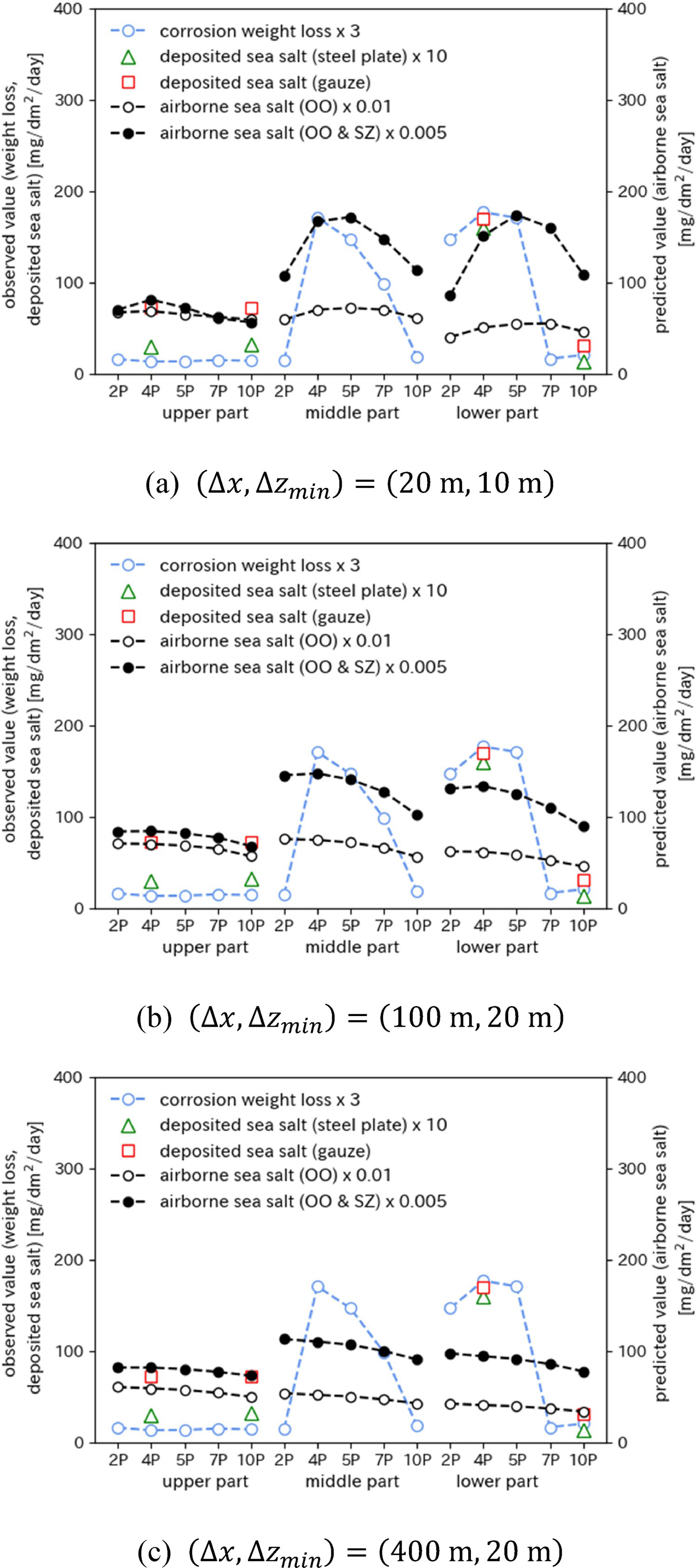
Regarding the effects of the grid spacing, the reproducibility of the local variation decreases with increased grid spacing. This is related to the distance between points 2P and 10P of ∼300 m. Although the variation in the vertical direction is measurably expressed even in the case of when SZ is considered, there is a tendency to underestimate the relative amount of airborne sea salt near the ground surface along the coast. This is apparent for the values at the lower part at point 4P in cases of lower grid resolution, for example.

The predicted and observed values at each observation point in Ozu are shown in Figure 11. The observation points are arranged in order of distance from the coast (L) on the horizontal axis. The predicted values are the amount of airborne sea salt for the OO only and the OO + SZ at a ground height of 10 m at each observation point. Note that the predicted values for the different ground heights of 5, 10, and 20 m exhibit a similar relationship to the observed values in a preliminary comparison. This suggests that the variation in the vertical direction becomes smaller than that in the horizontal direction in inland areas. It is apparent that consideration of SZ increases the amount of airborne sea salt when is <5 km, and it seems that the results for the OO + SZ are more closely correlated with the observed values. Note that the ratios of the OO values to the values for the OO + SZ at points with (∼0.5; see relevant legend) are within the range of the predicted results shown in Tedeschi et al. [15]. The small variation in the predicted values at close to the coastline is affected by the grid resolution.

Figure 11

Predicted and observed values at Ozu observation points (, ss: sea salt).

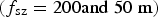The relationship between the predicted and observed values for Ozu is shown in Figure 12. The values at the points with and are represented by filled and unfilled plots, respectively. The regression lines and their coefficients of determination (R ²) for the points with are shown in the figure. Positive correlation was found. In particular, the R ² increased with increasing line gradient when the SZ particles were considered. The set value had little effect on the correlation, although it slightly altered the amount of airborne sea salt.

Figure 12

Relationship between the predicted and observed values for Ozu (lines: regression lines for points of , filled circles: values at points of , open circles: values at points of ).

For the points with , the tendency towards small variations in the predicted values were apparent again. This corresponds to the underestimation tendency near the coastal area ground surfaces under low grid resolution shown in Figure 10. It can be concluded that a high grid resolution enables the capturing of the spatial variation in the airborne sea salt in coastal areas.

Characteristics of ocean- and surf-originating particles transported inland

The characteristics of sea-salt particles transported inland according to their origin and size are discussed in this section. Figure 13 shows the mass fractions of particles with different sizes and origins in the annual mean amount of airborne sea salt at observation points in Ozu. The horizontal axis is L, which replaces the observation point numbers arranged in order of distance in Figure 11. The fraction of SZ particles dominating the amount near the coast decreases inland but does not become zero even at L > 5 km; this indicates that a portion of the SZ particles reaches inland, corresponding to the results of Tedeschi et al. [15]. Moreover, the decrease in the SZ particle fraction with increasing L is large for particles of class P3 with large size, showing that the larger SZ particles have a lower tendency to reach inland. Further, the results confirm that the SZ particle fraction decreases when smaller values are set.

Figure 13

Mass fractions of particles with different sizes and origins in the annual mean amount of airborne sea salt at Ozu observation points.

The particle size is a parameter that essentially affects the deposition efficiency (e.g. [27]), though the efficiency was simply assumed to be constant in this study. Considering that the fractions of differently sized particles vary with L, the estimation of the cumulative amount of airborne sea salt originating from both the OO and the SZ should lead to more accurate predictions for the absolute amount of deposited sea salt on the surfaces of structures at any location.

Conclusions

We estimated the spatial distributions of the cumulative amount of airborne sea salt originating from the open ocean (OO) and surf zone (SZ) using a method combining CFD simulation and a statistical method. A new method for predicting the SZ-originating particle concentration was incorporated. The prediction accuracy was evaluated by comparing the predicted amount of airborne sea salt with the observation data, and the characteristics of sea-salt particles with different origins and sizes transported inland were discussed based on the prediction results. The main findings are as follows.

Consideration of the SZ particles had a considerable effect on the prediction accuracy.

A high grid resolution was particularly conducive to the CFD simulation that capture the spatial variation in the amount of SZ airborne sea salt in coastal areas accurately.

The SZ width affected the absolute amount of airborne sea salt but had a smaller effect on the relative correspondence with the observed deposited sea-salt value.

The SZ sea-salt particles increased the amount of airborne sea salt in coastal areas and possibly reached inland for more than 5 km; this finding supported the results of Tedeschi et al. [15]. The larger SZ particles had a lower tendency to reach inland.

These findings suggest that considering the SZ particles must contribute to an improved prediction of the deposited sea salt on structures at any locations and will lead to an increased efficiency of maintenance activities and to an increased effectiveness of design and materials selection to combat corrosion. On the other hand, significant uncertainty remains in the prediction for the airborne sea salt (‘Accuracy evaluation’). One of the sources for this uncertainty is that the model parameters for predicting the SZ particle concentration are defined according to the limited available observation data and existing models (‘Concentration of particles reaching the coastline’). As a topic of future research, more appropriate methods for assessing the concentration and particle size distributions of SZ particles at the coastline should be developed, through a series of validation studies.

Footnotes

Acknowledgements

The authors acknowledge Shikoku Electric Power Co. for providing observation data. The authors are grateful to Professor K. Fujii, Professor H. Nakamura (Hiroshima Univ.), and the electric power companies of Japan for their invaluable advice and fruitful discussion. The authors also thank Dr N. Tanaka (CRIEPI) for his significant contribution to the initial development of this method and Mr K. Kanzaki (DCC) for his assistance in performing the numerical simulation.

Disclosure statement

No potential conflict of interest was reported by the authors.

References

Feliu

Morcillo

Chico

Effect of distance from sea on atmospheric corrosion rate. Corrosion. 1999; 55 (9): 883–891.

Obata

Watanabe

Guotai

. Numerical simulation of adhesion of sea-salt particles on bridge girders. Struct Infrastruct Eng. 2014; 10 (3): 398–408. doi: 10.1080/15732479.2012.757328

Fuse

Naganuma

Fukuchi

. Underfilm corrosion of transmission tower cross-arms service-used in a Pacific coast area. Corrosion. 2015; 71 (11): 1387–1397. doi: 10.5006/1736

Lee

J-S

Moon

H-Y.

Salinity distribution of seashore concrete structures in Korea. Build Environ. 2006; 41: 1447–1453.

Meira

Andrade

Padaratz

. Measurements and modelling of marine salt transportation and deposition in a tropical region in Brazil. Atmos Environ. 2006; 40: 5596–5607.

Manders

AMM

Schaap

Querol

. Sea salt concentrations across the European continent. Atmos Environ. 2010; 44: 2434–2442.

Woodcock

AH.

Salt nuclei in marine air as a function of altitude and wind force. J Meteor. 1953; 10: 362–371.

Toba

On the giant sea-salt particles in the atmosphere I. General features of the distribution. Tellus. 1965; 17 (1): 131–145. doi: 10.1111/j.2153-3490.1965.tb00202.x

Lewis

Schwartz

SE.

Sea salt aerosol production: mechanisms, methods, measurements, and models – a critical review. Washington (DC): American Geophysical Union; 2004. (Geophysical Monograph Series, 152).

10.

O'Dowd

de Leeuw

Marine aerosol production: a review of the current knowledge. Philos Trans R Soc A. 2007; 365: 1753–1774.

11.

de Leeuw

Andreas

Anguelova

. Production flux of sea spray aerosol. Rev Geophys. 2011; 49: RG2001.

12.

de Leeuw

Neele

Hill

. Production of sea spray aerosol in the surf zone. J Geophys Res. 2000; 105 (D24): 29397–29409.

13.

Clarke

Owens

Zhou

An ultrafine sea-salt flux from breaking waves: implications for cloud condensation nuclei in the remote marine atmosphere. J Geophys Res. 2006; 111: D06202.

14.

van Eijk

AMJ

Kusmierczyk-Michulec

Francius

. Sea-spray aerosol particles generated in the surf zone. J Geophys Res. 2011; 116: D19210.

15.

Tedeschi

van Eijk

AMJ

Piazzola

. Influence of the surf zone on the marine aerosol concentration in a coastal area. Boundary Layer Meteorol. 2017; 163 (2): 327–350.

16.

Suto

Hattori

Hirakuchi

. Computational fluid dynamics simulation and statistical procedure for estimating wide-area distributions of airborne sea salt considering local ground conditions. Struct Infrastruct Eng. 2017; 13 (19): 1359–1371.

17.

Lewellen

Sheng

YP.

Modelling of dry deposition of SO₂ and sulphate aerosols. Palo Alto (CA): Electric Power Research Institute; 1980. (EPRI EA-1452, project 1306-1, 68).

18.

Schlichting

Gersten

Boundary layer theory (8th revised and enlarged edition). Berlin: Springer; 2000.

19.

Suto

Kihara

Hattori

. Study on estimation of salt deposition with numerical simulation of sea salt particle transport (Part 8) – Development of estimation method for airborne sea salt originated from surf zone. Tokyo: CRIEPI; 2019. (CRIEPI Research Report, N19005).

20.

Kihara

Hirakuchi

Takahashi

. Numerical study on sea salt depositions in Niigata prefecture, Japan. Proceedings of the 7th Asian Aerosol Conference. Xian: Aerosol and Air Quality Research; 2011.

21.

Ohba

Okabayashi

Yamamoto

. A method for predicting the content of sea salt particles in the atmosphere. Atmos Environ. 1990; 24A (4): 925–935. doi: 10.1016/0960-1686(90)90295-X

22.

Hashimoto

Hirakuchi

Tamura

. A 53-year reproduction run over Japan using a regional climate model. Tokyo: CRIEPI; 2013. (CRIEPI Research Report, N13004).

23.

Fujii

Nakamura

Yamaguchi

. Corrosion phenomena caused by sea-salt particles on the original Amarube trestle bridge and applicability of the sea-salt transport model in a corrosion hazard assessment. J Jpn Soc Civil Eng Ser A1. 2017; 73 (1): 98–113.

24.

Chisholrn

Buchan

Jarv

Accurate measurement of low insulator contamination levels. IEEE Trans Power Delivery. 1994; 9 (3): 1552–1557.

25.

Monahan

Spiel

Davidson

KL.

A model of marine aerosol generation via whitecaps and wave disruption. In: Monahan

Niocaill

, editors. Oceanic whitecaps. Oceanographic Sciences Library, Vol. 2. Dordrecht: Springer; 1986. p. 167–174.

26.

Slinn

WGN.

Predictions for particle deposition on natural waters. Atmos Environ. 1980; 14: 1013–1016.

27.

Poots

Ice and snow accretion on structures. Hoboken (NJ): John Wiley and Sons Inc; 1996.