The Role of Working Memory in Information Acquisition and Decision Making: Lessons from the Binary Prediction Task

Abstract

The effects of memory constraints upon information acquisition and decision making were examined in two experiments using binary prediction tasks, where participants observe outcomes for two options before deciding which one to bet upon. Our studies extend previous investigations to the case where participants learn the structure of the task through observation, but where information acquisition is separated from the task of prediction. Participants with higher cognitive capacity (larger memory span or higher intelligence) were more likely to adopt the “maximizing” strategy (always selecting the more frequent alternative). This finding conflicts with some recent investigations of similar tasks, a contrast that implies that the presence of feedback on choices may be important in determining the strategic actions of high-capacity individuals. Participants selecting the optimal strategy were in turn more efficient in their data acquisition. The behaviour of participants adopting suboptimal choice strategies was consistent with prediction based upon a “narrow window of experience”—that is, seeking to match the characteristics of small samples of observations.

Keywords

Choice Probability Binary prediction Information acquisition Memory Working memory Intelligence

This paper reexamines the binary prediction task—a simple, yet deceptively rich, experimental task—where participants acquire information and make multiple choices. Our particular focus is on how constraints in the capacity of short-term or working memory impinge upon information acquisition and choice. Our introduction begins with an outline of the binary prediction task. Then, we consider how memory processes relate to information acquisition and decision making from which we identify the key questions of our investigation.

The Binary Prediction Task

The binary prediction (BP) task is a simple choice task under uncertainty, which involves learning from experience which of two mutually exclusive and exhaustive outcomes is more likely and deciding which one to bet upon. Early versions of the task (which have become the model for many subsequent instantiations of the task) presented participants with two light bulbs (A and B), one of which would light up on each of the many trials in the experiment (e.g., Goodnow, 1955; Humphreys, 1939). The probability with which Bulb A would come on was set to probability p across all trials; therefore Bulb B lit up with probability (1 – p). Participants were required to predict on every trial which light would come on. Correct predictions were rewarded (e.g., with 5¢), whereas incorrect predictions either received nothing or were penalized (e.g., lose 5¢) depending upon the pay-offs chosen by the experimenter (Bereby-Meyer & Erev, 1998; Brackbill, Kappy, & Starr, 1962). Thus participants could use information acquired on previous trials to guide subsequent choices.

An alternative of the task is reported by Tversky and Edwards (1966). Their participants chose between three (rather than two) courses of action on each trial: (a) Observe which of the two lights comes on, (b) predict that the left light will come on, or (c) predict right. Participants received 5¢ for a correct prediction or lost 5¢ if they were incorrect, but received no feedback as to which light came on. Thus the only way to learn about the task was to select Action 1 (observation). This procedure was repeated for 1,000 trials, for which the probability of the more frequent alternative was fixed: either at .7 or at .6 (between subjects). We call this version of the BP task the “observe-or-bet” task, and we adopt it for our investigation as it neatly separates, and clearly defines, the information acquisition and choice components of the task. The task also reflects the many instances in everyday life where we do not receive immediate feedback on our decisions (Elwin, Juslin, Olsson, & Enkvist, 2007; Hogarth, 2006).

It is possible to prescribe what participants should do in the observe-or-bet task. By increasing the number of observation trials, one obtains increasingly reliable information about which light is the more frequent alternative. However, this information is costly, as on any observation trial one forgoes the opportunity to earn money. For specified pay-offs, one can calculate the optimal number of observation trials in order to maximize expected winnings. Once these observations have been made, thereafter, participants should commit themselves to predicting the more likely outcome for the remaining trials. Always predicting the most commonly observed outcome is optimal in any variant of the BP task (if participants are told that the probability of each alternatives is fixed across trials). Hence selecting the more frequent alternative is often referred to as making a “maximizing choice”, and doing so consistently is termed “maximizing”. Tversky and Edwards (1966) reported three ways in which their participants’ behaviour was suboptimal.

First, participants observed for many more than the optimal number of trials—approximately 10 times as many as the optimal number of observations. Second, they distributed their observations across the 1,000 trials, as opposed to massing their observations at the start. Thus, on early trials they committed themselves to predictions without the benefit of all the predecisional information that they eventually acquired. Third, they distributed their predictions between the two lights, rather than betting only on the more frequent alternative. Many participants placed bets roughly in proportion to what they had observed, for instance betting right 70% of the time and left 30% of the time when the right-hand light is set to come on with probability .7. This pattern of prediction, which is termed probability matching, yields accuracy below the 70% that would be achieved by always betting on the more frequent alternative: expected proportion correct = (.7×.7) + (.3×.3) = .58. Many other BP studies report overmatching: betting upon the more frequent alternative at a rate slightly higher than its relative frequency (which is still suboptimal). In fact, as long real stakes are used (Brackbill et al., 1962), overmatching seems to be the norm no matter how the game is presented (Fantino & Esfandiari, 2002; Goodnow, 1955; Nies, 1962; Peterson & Ulehla, 1965).

Memory Constraints in Information Acquisition

Memory ought to play a particularly important role in tasks, like the BP task, that require active information acquisition prior to choice. Collecting and collating the information about the options place demands upon memory, and choices are based on memorized information.

Kareev has put forward a narrow window hypothesis of data sampling for tasks involving sequential information acquisition (Kareev, 1995a, 1995b, 2000; Kareev, Lieberman, & Lev, 1997). Kareev appeals to the observation, first popularized by Miller (1956), that the amount of information that we can process on a single dimension is limited to about seven items, and the number of objects that we can hold in working memory at any one time is about seven “chunks” of data. He proposes that judgements are based on small samples of around seven exemplars from the observed sequence. Perhaps counterintuitively, and certainly controversially (Anderson, Doherty, Berg, & Friedrich, 2005; Juslin & Olsson, 2005; Kareev, 2005), Kareev proposes that this limitation affords humans an advantage in the early detection of correlation, especially for pairs of dichotomous variables. Small samples tend to amplify correlations as the sampling distribution for a correlation coefficient is biased, having a median and mode more extreme than the population value. Kareev supports his view with two experiments, in which he inferred the detection of correlation from predictions of the next item in a sequence of observations, with feedback given on every trial (Kareev et al., 1997). In Experiment 1, participants with lower immediate memory capacity (assessed by digit span) were more accurate in assessing the association between the colour of an envelope (red or green) and the symbol assigned to a coin hidden inside the envelope (“X” or “O”). In Experiment 2, the assessment of correlation was more effective when participants were presented with smaller, rather than larger, samples (when presentation was sequential).

Gaissmaier, Schooler, and Rieskamp (2006) note that Kareev's envelope task is a type of BP task. To maximize the financial rewards of the experiment, participants should always predict whichever symbol is more common for a given colour of envelope. Thus, greater extremity in the (inferred) estimation of correlations among low-memory-span participants equates to more maximizing choices for these participants. Using a very similar paradigm, Gaissmaier et al. partially replicated this advantage in maximizing choices for low-span participants in the initial stages of the task, but found a tendency towards a high-span advantage when the contingency between colour of envelope and symbol changed part way through the task. Gaissmaier et al. propose that low memory capacity may not be advantageous for detecting correlation. Rather these participants prefer a simple initial response to the problem (of always predicting the same outcome) and are slow to change their predictions when conditions change. In contrast, individuals with higher cognitive capacity actively (though erroneously it turns out) search for patterns. This drives them towards suboptimal matching-type behaviour, but does mean that they are more likely to attend to, and therefore to respond to, changes in the environment. This tendency to treat the BP task as a problem-solving exercise and search for (illusory) patterns in the sequence of lightings is seen in other BP investigations (Newell & Rakow, 2007; Wolford, Newman, Miller, & Wig, 2004) and may be attributed to representative reasoning about the sequences (Kahneman & Tversky, 1972).

The paradigm employed by Kareev et al. (1997) and Gaissmaier et al. (2006) does have some drawbacks when it comes to investigating the impact of memory constraints upon information acquisition (though some testable predictions, as described above, can be made). As data are acquired, and predictions are made on every trial, it is difficult to obtain a direct measure of the amount of information that has been sampled or attended to. The observe-or-bet BP task that we employ is arguably more suited to this, as we can record how many observations a participant makes before making a choice or series of choices. Kareev's theory speaks to samples held in working memory, which are most likely to include recent observations but may also include more distal observations that are retained in long-term memory. However, the observe-or-bet task allows us to ask whether the narrow window hypothesis predicts how much information participants choose to acquire. The most straightforward prediction on the basis of the narrow window hypothesis is that participants with lower memory capacity will collect less predecisional information (or at least collect less during any one period of continuous observation).

Memory Constraints in Decision Making

A different line of enquiry into optimal behaviour in BP tasks has investigated choice strategies in simple word-based probability problems. For example, Gal and Barron (1996) and West and Stanovich (2003) presented participants with the following “die problem” version of the BP task. A die, having four red faces and two green faces, is rolled repeatedly. A prediction of what colour will show is made before each roll, with a prize for a correct prediction. Participants were then asked to endorse one of (or to rank) a number of discrete strategies, which included maximizing (always selecting the most frequent option) and matching (predicting in keeping with the 2:1 ratio of the two colours). West and Stanovich found that participants who endorsed the maximizing strategy in the die problem and in a similar trial-by-trial card game (with event probabilities specified) had significantly higher Scholastic Assessment Test (SAT) scores than students selecting other strategies, though did not have more quantitative or statistical training. Gal and Baron (1996) found that sixth- and ninth-grade students endorsed matching more frequently and maximizing less frequently than their college sample. Derks and Paclisanu (1967) found an equivalent trend for more optimal responding with increasing age (from kindergarten to college) with a trial-by-trial task, with the striking exception that nursery children were most likely of all to maximize (perhaps reflecting a preference for “simple” responding). West and Stanovich (2003) argue that, like intelligence tests, SAT scores assess general cognitive ability. They conclude that participants of greater cognitive ability are more likely to override the intuitive seduction of matching based on heuristic reasoning about local features of the problem and to adopt the optimal strategy based on normative reasoning about long run or independent outcomes.

The positive correlation between general cognitive capacity (e.g., as assessed by intelligence tests) and working memory capacity is well established (Daneman & Merikle, 1996; Engle, Tuholski, Laughlin, & Conway, 1999). Indeed, memory span measures are included in some test batteries for general intelligence, and some have proposed that working memory capacity is the major determinant of reasoning ability or intelligence (Kyllonen, 1996). Successful reasoning and decision making often involve acting upon several items of information simultaneously (e.g., attending to information whilst selecting a course of action), a task that should be performed less successfully by those with low memory spans who can consider only a limited amount of information. Stanovich and West (2000) argue robustly for this position and identify many failures in reasoning, judgement, and decision making that are associated with lower intelligence or lower working memory capacity.

Summary of Predictions

Our task differs in potentially important respects from prior studies of the relationship between cognitive capacity and BP performance. In contrast to Gal and Barron (1996) and West and Stanovich (2003), our participants must learn which option is more probable (and how probable) by observation. But, unlike Kareev et al. (1997) and Gaissmaier et al. (2006), our participants do not receive feedback on their predictions (thereby separating the actions of information acquisition and prediction). Thus there is some conflict in what we should expect in the observe-or-bet BP task. The narrow window hypothesis predicts more extreme responses (more maximizing) when memory capacity is low. We might also expect to see lower levels of information acquisition when memory capacity is low—though this is not critical to the narrow window hypothesis. In contrast, the close relation between memory capacity and decision-making ability and the findings of Gal and Baron (1996) and West and Stanovich (2003) would lead one to expect more successful responding (more maximizing) when memory capacity is high.

Experiment 1: Memory Capacity and Binary Prediction

In this first experiment we use an observe-or-bet BP task similar to Tversky and Edwards (1966) to examine information acquisition and choice behaviour in a task where the probabilities of the (two) outcomes are learned by experience. Participants also completed the die problem described above. In order to investigate the role of memory constraints, participants completed a battery of memory tasks. The different tasks assessed memory capacity according to one of two alternative conceptions of the “size” of memory: (a) the storage capacity of the short-term memory store (“pure memory span tasks”), or (b) the storage plus processing capacity of working memory (“working memory span tasks”).

This follows the pattern of a number of studies that have examined which of these two conceptions of memory capacity (pure span or working memory span) best predicts performance in a variety of cognitive tasks (Conway et al., 2005; Daneman & Merikle, 1996; Engle, Nations, & Cantor, 1990). Our purpose in this is exploratory, but it does offer the opportunity to learn more about the precise role of memory constraints in this task. If short-term memory is constrained purely by the “number of slots” available in memory or the “size of the window” of conscious attention, then the narrow window hypothesis would predict that individuals with larger short-term memory capacity (as measured by pure memory span tasks) should sample more information before making a decision. However, if one also considers the processing limitations of working memory then one might predict that in order to reach a given diagnostic threshold for choice, an individual with a limited working memory will sample more predecisional information than someone who has a better (i.e., more efficient) memory. In other words, the ability to extract information from data (cf. Edwards, 1965) would correlate positively with working memory capacity.

Method

Participants

The participants were 24 members of the University of Essex community (10 males; 12 native English speakers). The mean age was 25.7 years (SD 8.1, range 19–54).

Tasks

The Binary Prediction (BP) Task

This task comprised a series of games, each game consisting of 100 trials. On each trial, participants saw two light bulbs represented on the monitor screen, one on the left side and one on the right side of the screen. On every trial one of the light bulbs was programmed to light up—therefore, participants observed a pair of mutually exclusive and exhaustive events on each trial. The probability with which each bulb lit up was fixed throughout each game, but varied from game to game (of which participants were made aware). On each trial, participants could observe which bulb lit up without cost, or could choose to predict which light bulb would light up (in which case they received no feedback on that trial). On any trials for which a prediction was made, participants won 3p (approximately 5 US or euro cents at the time of testing) if their chosen bulb lit up, but lost 3p for an incorrect prediction. Thus participants controlled the number of observation trials and would expect to be in profit for the game if they bet on some trials and chose the more frequent alternative more than the less frequent one. Additional observations improve the chances of correctly identifying the more frequent alternative, but forgo the opportunity to earn money.

The probability of the more frequent alternative varied across the six games, between p = .55 and p = .80 in increments of .05. These six contingencies were preprogrammed as random sequences of the appropriate number of “lightings” of the more frequently lighting bulb (e.g., 70 out of 100 when p = .70). For a given game the same randomly determined left–right sequence was employed, for which it had been determined at random whether the right or the left bulb was the more frequent one. Games were placed in a single randomly determined sequence but the order of this sequence (forwards or backwards) was counterbalanced using random allocation across participants (p = .65 was first in backwards order, and last in forwards order; p = .80 was first in forwards order, and last in backwards order). To maintain motivation and reward optimal behaviour, participants were paid their winnings.

Memory Tasks

A battery of eight standard memory tasks was administered (see Appendix for full details). This permitted more reliable assessment of memory capacity than previous similar investigations (Gaissmaier et al., 2006; Kareev et al., 1997) and allowed consideration of two components of memory capacity: storage and processing efficiency. Four tasks were ones that are conventionally considered to assess the pure storage capacity of short-term memory (Daneman & Merikle, 1996): word span and digit span, each assessed forwards and backwards. We refer to these as short-term store (STS) tasks. Four tasks were ones that are used to assess both the storage capacity and the processing capacity of short-term memory (Daneman & Merikle, 1996): working memory for numbers, words, sentences, and an operations span task. These tasks require participants to retain items in memory whilst processing information, which we refer to as working memory (WM) tasks. All tasks were computer controlled, stimuli were presented on screen, and participants gave their response out loud (to be recorded and scored by the experimenter).

Die Problem Questionnaire

Participants completed the die problem (West & Stanovich, 2003; adapted from Gal & Baron, 1996). Participants were asked to imagine a die with four red faces and two green, to be rolled 60 times. Participants specified which strategy they would use to make the most money if they won £1 each time they correctly predicted the colour of the die in advance of each roll. Five strategies were listed: predicting the most likely outcome on every roll (the maximizing strategy), predicting according to the ratio of red and green faces (matching), and three strategies reflecting the gambler's fallacy.

Apparatus

The tasks (for this and for Experiment 2) were written in the REALBasic language with the appearance of a “Windows-type” environment and were run on the Apple eMac G4 computers.

Procedure

Participants were tested individually in a session that lasted approximately 90 minutes, beginning with the BP task. The instructions for the BP task were provided on screen, though the experimenter remained with participants until they had begun the task (to ensure adequate understanding). The instructions familiarized participants with how the three possible actions (observe, predict left, or predict right) were made. Participants were also informed that the probability with which each bulb lit was fixed for the entire game, but could vary from game to game—and were reminded of this by a “message box” that appeared between successive games. Winnings from each game were only revealed once all six games were completed. The memory tasks were then administered in the order listed above. (As we were interested in the correlation rather than the difference between measures, it was felt unwise to counterbalance the order of tasks, as any fatigue or practice effects would then have differential impact upon a given task.) Finally, participants completed the die problem, provided demographic information, and were paid their turn up fee of £6 plus their additional winnings from the BP task.

Results and Discussion

For each game, several measures were obtained for every participant. The measures of information acquisition included the number of observation trials (/100) and the number of observation sequences (an observation sequence being any stream of one or more observation trials uninterrupted by a prediction trial). Other measures of process were the mean reaction time (in seconds) and the number of action changes (the number of consecutive trials that did not have the same one of the three possible actions: observe, predict left, or predict right)—the latter measure reflecting the extent to which participants “flip-flop” between possible actions. A further measure was computed: the mean length of observation sequence (=number of observation trials/number of observation sequences).

Accuracy or appropriateness of responding was measured by the proportion of prediction trials in which the more frequent alternative was chosen, the proportion correct, and winnings (in pence). Also, each game was coded according to whether a participant adopted a strict maximizing strategy (picking the same alternative on every bet trial), from which we computed the number of games (/6) for which each participant adopted this strict maximizing strategy.

The Relationship between Memory Measures and Performance on the BP Task

Each of the process measures (excluding winnings and accuracy, which are subject to a random component) had good reliabilities (minimum Cronbach's α of .67, median of .90). Participants’ strategies were therefore highly consistent—for example, those with more observation sequences in one game tended to have more observation sequences in other games. Means were created for each participant for each of the process measures (i.e., collapsing across games) to facilitate examination of BP task behaviour and memory performance.

Scores on the four STS span tasks were positively correlated and were averaged to provide a single STS measure (α = .66). Performance on the WM operations task was uncorrelated with the other WM tasks. Therefore, the WM operations task was treated separately, but scores on the other three WM tasks did correlate positively and were averaged to create a single WM score (α = .79). Because some of the memory tasks depend upon verbal fluency, we first examined whether there was any effect of native language upon the memory measures. Mean STS (maximum possible = 14.5) did not differ between native and non-native English speakers (M = 7.02 vs. 6.96), t(22) = 0.10, p = .918. Mean WM score (maximum possible = 42) was significantly higher for native English speakers (M = 36.2 vs. 30.0), t(22) = 3.53, p = .002. Mean WM operations score (maximum possible = 42) was lower for native English speakers, and the difference approached significance (M = 23.2 vs. 29.4), t(22) = 1.88, p = .074. Therefore, when examining correlations between measures, we partialled out native language. We also excluded one extreme outlying participant, who had observed on nearly every trial, from our correlational analyses because of the difficulty of interpreting correlations involving his/her mean length of observation sequence.

A number of key tendencies in information acquisition and choice behaviour are evident in Table 1. With respect to choice behaviour, those with higher WM scores pick the better alternative more often. Higher STS and WM scores both predict more frequent use of a strict maximizing strategy. This positive relationship between memory capacity and maximizing is in keeping with West and Stanovich (2003) and Gal and Baron (1996; see also Stanovich & West, 2000) and contrasts with the findings of Kareev et al. (1997) and the predictions of the narrow window hypothesis. More frequent use of the maximizing strategy is associated with fewer action changes (inevitably), with picking the better alternative more often (as per the structure of the task), and with quicker reaction times (presumably because participants are committed to a repetitive or simple strategy). Choosing more quickly when maximizing is also consistent with threshold models of choice (e.g., Busemeyer & Townsend, 1993): stronger preferences between options being consistent with reaching a decision threshold more quickly. Interestingly, more frequent maximizing is only minimally associated with less observation.

Table 1

Experiment 1: Partial correlation between BP task measures and memory measures

	2. WM	3. WM operations	4. No. obs. trials	5. No. obs. sequences	6. Length obs. sequence	7. RT	8. No. action changes	9. Prop'n better alt've	10. No. BP max strategy games	11. Winnings	12. Max strategy on die problem
1. STS	.38⁺	.53^*	−.32	−.32	.09	−.49^*	−.48^*	.03	.45^*	.34	.33
2. WM span		.15	.03	−.14	.18	−.62^**	−.50^*	.50^*	.48^*	.58^**	.52^*
3. WM operations			−.22	−.46^*	.28	−.27	−.37⁺	−.33	.04	.02	.28
4. Number of observation trials				.50^*	−.16	.38	.20	.33	−.27	−.44	−.05
5. Number of observation sequences					−.69^***	.37+	.72^***	.23	−.17	−.37⁺	−.26
6. Length of observation sequence						−.24	−.45^*	.03	.09	.31	−.08
7. RT							.55^**	−.21	−.46^*	−.59^**	−.27
8. Number of action changes								−.25	−.51^*	−.56^**	−.55^**
9. Proportion of times better alternative is picked									.47^*	.55^**	.35
10. Number of BP maximizing strategy games										.64^**	.47^*
11. Winnings for BP task											.40⁺

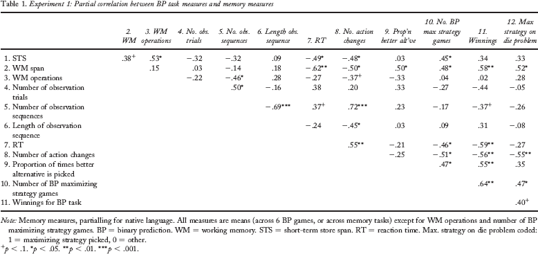
Memory measures, partialling for native language. All measures are means (across 6 BP games, or across memory tasks) except for WM operations and number of BP maximizing strategy games. BP = binary prediction. WM = working memory. STS = short-term store span. RT = reaction time. Max. strategy on die problem coded: 1 = maximizing strategy picked, 0 = other.

p < .1.

p < .05.

p < .01.

***

p < .001.

With respect to information acquisition, it would appear that memory capacity has a closer relation to the process or distribution of sampling than to the gross amount of information acquired. Those with better memory performance are quicker at the task, make fewer action changes, and make slightly fewer sequences of observations. This may well be because participants with greater memory capacity were more likely to be those who committed themselves to the simple and repetitive maximizing strategy, which reduces alternation between options and allows fast responding. There was no significant correlation between the memory measures and the number of observation trials or the length of observation sequence. However, there was a minimal tendency for longer observation sequences among those with greater memory capacity in keeping with our conjectured extension of the narrow window hypothesis. The predictive power of the WM and STS measures is similar: Both storage capacity and processing efficiency predict patterns of information acquisition.

Maximizing Strategies

The frequency of strict maximizing in the observe-or-bet task increased steadily with increasing probability of the more frequent alternative: from one participant when p = .55, to 11 participants when p = .80. There was also some indication that strict maximization became more likely with increasing task experience. A total of 9 of the 11 participants who maximized when p = .80, and 3 of the 4 who maximized when p = .65, experienced this as their last game rather than their first game. This influence of contingency (the probability of the more frequent alternative) and experience upon the amount of maximizing is examined more thoroughly in Experiment 2, where game order and contingency are fully counterbalanced (rather than partially as was the case here).

A total of 8 of the 24 participants identified the maximizing strategy (always pick the more frequent colour) as the best strategy in the die problem, and 16 picked other strategies (mostly matching). Those that endorsed maximizing in the die problem had maximized more frequently in the preceding BP task than other participants (on 44% vs. 16% of games). Thus, strategy preference on a BP task that is described to participants but not played out with trial-by-trial predictions aligned with choice strategy in a similar (though not identical) BP task in which participants acquire information sequentially and can make trial-by-trial predictions.

Predictors of Adopting a Maximizing Strategy (BP Task and Die Problem Questionnaire)

We examined which variables might predict optimal strategy selection—that is, strict maximizing behaviour in the computerized BP task and selecting the maximizing strategy in the die problem. The tendency to adopt a maximizing strategy was not enhanced by greater experience with mathematics/statistics.

As identified above, participants with greater STS and WM capacity maximized more often in the BP task (r = .45 and .48, respectively). The final column of Table 1 also shows a tendency for those with better scores on the memory measures to pick the maximizing strategy in the die problem more frequently (large significant effect for WM and medium nonsignificant effect for STS and WM operations).¹ Note also that choice strategy is consistent across the two tasks: Die problem maximizers make significantly fewer action changes and adopt a strict maximizing strategy more often. Moreover, explicit endorsement of maximizing is associated with a more “efficient” approach to the task: These participants tend to earn more and respond more quickly.

To provide a more powerful analysis of this relationship, we combined these data with equivalent data from a subsequent experiment (not reported here) using another version of the BP task, where the same set of memory measures and the die game problem were used with the same subject pool (total n = 52). Mean memory scores were compared between participants selecting the maximizing strategy in the die game and those selecting another strategy. Mean STS was significantly higher for maximizers (M = 7.82 vs. 6.68), d = 0.72, t(50) = 2.30, p = .026, as was the case for WM score (M = 34.7 vs. 31.2), d = 0.67, t(50) = 2.16, p = .036. The difference for WM operations was also in this direction, but not significant (d = 0.39, p = .215). These results, are consistent with West and Stanovich's (2003) finding that higher cognitive capacity predicts selection of the maximizing strategy—and, like them, we found die problem maximizing to be more common among males than females (35% vs. 22% for the combined sample).

Key Findings from Experiment 1

We found that those with greater memory capacity tended to do better at the BP task: They were more likely to adopt a maximizing strategy (sticking to the same choice throughout) and, consequently, picked the better alternative more often and earned more money in the task. They also responded more quickly. Consistent with the relationship between memory capacity and strategy choice, those with greater memory capacity more readily identified the optimal strategy in the die problem. Thus, consistent with the views of Stanovich and West (Stanovich & West, 2000; West & Stanovich, 2003), we see a number of ways in which higher cognitive capacity is associated with more successful responding. This experiment suggests that cognitive limitations do not confer an advantage in this version of the BP task, contrary to the predictions of the narrow window hypothesis.

Experiment 2: At what Level do Memory Constraints Matter?

This second experiment was designed to resolve precisely what the role of memory is in the binary prediction task. In order to advance upon our correlational data on memory, in this experiment we manipulated memory capacity by means of a secondary task (counting tones whilst carrying out the observe-or-bet BP task). Our purpose was to determine why strategy selection is better among participants with higher WM capacity.

Several findings in the reasoning and problem-solving literatures point to a positive relationship between adaptivity in strategy selection and WM capacity (Dierckx & Vandierendonck, 2005). It would appear that a large WM capacity allows for success in selecting strategies for performing a task whilst performing the task itself—presumably because one has spare capacity to devote to strategy selection whilst simultaneously engaging in the task (Stanovich & West, 2000). Therefore, if the secondary task in this experiment degrades performance, it implies that strategy selection in the BP task is, at least in part, an “online” or concurrent process, which occurs in parallel with the acquisition of predecisional information. Additionally, if the rate with which participants switched to a maximizing strategy as the games progressed were greater for those without a secondary task, this would further support the spare capacity argument.

Alternatively, the memory demands of actually undertaking the BP task may be incidental to the relationship between memory capacity and BP task performance. For instance, those with greater memory capacity may work out from the task instructions what the optimal “maximizing” strategy is (see West & Stanovich, 2003) and then set themselves the relatively simple task of determining which light is more frequent in order to implement this strategy. In this case, a secondary task would not be expected to affect strategy selection in the BP task. Indeed, it may be that other components of intelligence, which nonetheless correlate with memory capacity, are the key determinants of the improvements in BP task performance with increasing memory capacity. For this reason, an IQ measure was also included in Experiment 2.

Thus, Experiment 2 reexamines the observe-or-bet BP task, requiring some participants to carry out the task with a secondary task (counting tones) that loads working memory. This is compared with two control conditions: one where participants hear the same tones as in the memory load condition but are instructed to ignore them (a distractor condition); and one without tones (i.e., like Experiment 1).

Method

Participants

A total of 56 first-year psychology students from the University of Essex participated (15 males), with a mean age of 19.3 years (SD 2.5, range 18 to 29). Non-native English speakers were excluded from participating to avoid having to partial out language in analyses involving memory measures.

Tasks and Design

The observe-or-bet BP task as used in Experiment 1 was used for this experiment. The following adaptations were made to permit a detailed and controlled consideration of the effect of task experience. Each participant in a given condition experienced the games in a unique order, determined by a series of Latin squares to ensure that each contingency was encountered with equal frequency across the six game positions. Different sets (six contingencies: p = .55 through p = .80) of randomly determined orderings of the two alternatives were created for the 100 trials, with each group of 6 participants (sharing the same Latin square) sharing the same set of orderings. These sets (determined by the ordering of games and the sequences of outcomes) were used for each condition of the experiment. Thus, the characteristics for a given participant were matched to those for another participant in each of the other conditions. As in Experiment 1, sequences were fixed so that the relative frequency of events matched the designated contingency. The bulb (left or right) that was the more frequent alternative was randomly determined on each game.

Participants were randomly allocated to one of three conditions: memory load (ML), distractor, or no load (NL). In the ML and distractor conditions, a 500-ms tone sounded on each trial. The tone began 750 ms after the participant had selected their chosen action (predict left, predict right, or observe). The tone was either high frequency (400 Hz) or low frequency (250 Hz), with the tone frequency (high or low) being selected randomly with probability .5 on each trial. ML participants were instructed to count the number of high tones that they heard during each game and to report this at the end of the game. Distractor participants were instructed to ignore the tones.

Three measures of cognitive capacity were obtained (either one or two weeks before, or immediately before the BP task was completed—these timings being unrelated to condition assignment). To measure memory capacity efficiently, participants completed only the WM words and forward digit span tasks, as these two tests best reflected the overall scores on the composite WM and STS measures in Experiments 1 (and in other studies in our lab). The shortest and longest digit strings (being uniformly easy and impossible to recall, respectively) were omitted from the digit span task, as these contributed nothing to the goal of discriminating between participants. Responses for these two tasks were recorded on tape and marked later by the experimenter. Participants also completed Raven's Advanced Progressive Matrices as a 40-minute timed test, administered as prescribed by the test manual. Raven's matrices is considered to be one of the best culture-free measures of g or general reasoning ability (Meo, Roberts, & Marucci, 2007). Obtaining these additional measures allowed us to examine the interplay between intelligence, memory capacity, and BP task performance.

Procedure

The participant instructions and procedure for the BP task were identical to those in Experiment 1. After these task instructions, participants in the ML and distractor conditions were also informed that they would hear a tone (either high or low) on each trial, and that “the tone that sounds has nothing to do with which bulb has lit up”. Participants in the distractor condition were told that they should do their best to ignore the tones whilst playing the games. Participants in the ML condition were told that, in addition to playing the (BP) games, they were to count the number of high tones to be reported at the end of each game. Before beginning the fist BP game, ML participants then played each tone a minimum of five times each to familiarize themselves with the difference between the tones. Participants received course credit for participating, but were also paid according to their performance in order to motivate their choices. Participants were informed immediately before reading the task instructions that their earnings on half of the games would be turned into actual payment, but (to maintain motivation) that they would not know until the end of the experiment which specific games this would be for. To enhance fairness, all participants received payment according to their performance on the p = .55, .65, and .75 games. At the end of the session, participants completed the die problem questionnaire and received their payment: mean £1.04 (approximately US$1.60 or 1.20 euro), range £0.00 to £2.30.

Results and Discussion

Due to technical difficulties with recording equipment, digit span scores were not obtained for 3 participants, and WM scores were unavailable for 4 participants. All other data were complete and were treated as per Experiment 1. Mean (SD) scores for the capacity measures were: 7.83 (1.72) out of 12 for digit span, 33.0 (4.5) for the WM score, and 22.6 (5.1) for Raven's matrices. As a check on our memory load manipulation, reaction times (RTs) were examined. As expected, RTs were slower and more variable in the ML condition, but (perhaps surprisingly) quicker in the distractor condition than in the NL condition (see Table 2). Consistent with this, factorial analysis of variance (ANOVA) with RT as the dependent variable and game number (i.e., 1 = first through 6 = last) and condition as the factors found a medium-sized effect of condition, η_p² = 0.105, F(2, 53) = 3.1, p = .054. Notably, the condition by game number interaction was significant, F(10, 265) = 2.6, p = .006, with η_p² = 0.088. Inspection of the relevant means indicates that, consistent with the secondary task serving to engage participants’ attention, initial responding in the ML condition is slower than that for the other two conditions, and that this gap decreases with practice. Thus in Game 1, mean RT in the ML condition was 40% higher than that in the other two conditions (combined), falling to 22% higher by Game 3 and 14% higher by Game 5. Accuracy on the tone counting task was good for most participants, implying proper engagement with the secondary task. The reported count was within 5% of the actual count in the majority of games (median absolute counting error or 2) and was within 10% or the true count in 3 out of 4 of the games.

Table 2

Experiment 2: Means for data averaged within participant by condition plus effect

Measure	Condition			Effect
Measure	Memory load	Distractor	No load	η²	F(2, 53)	p
Mean number of observation trials	29.3 (22.7)	32.2 (19.7)	27.7 (13.2)	.010	0.3	.762
Mean proportion of trials better option is picked	.69 (.14)	.72 (.12)	.74 (.15)	.039	1.1	.344
Mean reaction time (s)	0.84 (0.39)	0.63 (0.14)	0.75 (0.15)	.099	2.9	.094
Mean number of action changes	33.7 (18.2)	34.7 (20.4)	32.0 (17.5)	.004	0.1	.906
Mean number of observation sequences	7.8 (6.3)	10.8 (8.9)	8.1 (6.8)	.033	0.9	.414
Mean length of observation sequence	6.1 (4.3)	5.9 (4.6)	8.6 (8.5)	.040	1.1	.337
Number of strictly maximizing games	0.84 (1.34)	0.95 (1.78)	1.28 (1.84)	.013	0.3	.712
Total winnings (pence)	176 (172)	220 (136)	234 (148)	.027	0.7	.486

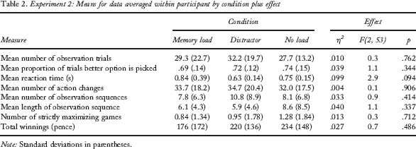
Note: Standard deviations in parentheses.

Table 2 gives an overview of the data, summarizing the data according to the mean scores of each participant for each of the measures of interest. This indicates minimal impact of condition upon measures reflecting data acquisition or choice. The only medium-sized effect of condition occurs for RT (see above). Condition was retained as a factor in the analyses of the effect of contingency and game number upon task performance that follow. However, as the effect of condition and the two-way interaction were at best small to medium in size and never significant, we do not report means separately by condition for these analyses.

Table 3 shows the data analysed by contingency (i.e., probability of the better alternative). As identified above, RT excepted, the effect of condition for all measures is small or small to medium in size and nonsignificant (all η_p² < 0.041, all F < 1.11, all p > .336). Similarly, all of the two-way (condition-by-contingency) interactions are of small or small-to-moderate effect size and are not significant (all η_p² < 0.046, all F < 1.24, all p > .267). However, Table 3 shows clear effects of contingency for a number of measures. The number of observation trials decreases with increasing contingency (large linear effect), markedly so for the highest two contingencies. Thus, consistent with normative considerations, fewer data are acquired when the difference between the alternatives is more clear-cut. Note that this seems to be predominantly achieved by a decrease in the length of observation sequence with increasing contingency (moderate effect for this linear trend), whereas the number of observation sequences does not alter systematically with the contingency. Thus it would seem that participants do not sample a constant amount of data: neither within any given period of observation, nor across the whole game. Note also that there is considerable between-participants variation for each of these three main indicators of data acquisition behaviour (listed first in Table 3). There is also a small-to-medium-sized (η_p² = 0.039) but statistically significant linear trend of contingency for reaction time, representing a slight tendency for quicker responding as the difference between alternatives increases (i.e., for increasing contingency). Thus, consistent with threshold models, response times decrease when the alternatives are more distinct/discriminable. Table 3 also shows a very strong effect of contingency upon choice behaviour. Mean choice proportions for the better alternative increase with contingency. When averaged across conditions, proportions are close to matching for p = .60, .70, and .80, overmatching by a little for p = .55 and .75, and slightly more so for = .65. The large standard deviations indicate that few individuals were close to matching the objective probability. Note also that the incidence of strictly maximizing choice (i.e., always select the same option) rises steadily with contingency: from around 10% of the time for p = .55 or.60 to about 25% for p = .75 or .80. A Cochran's Q test confirmed that these proportions vary significantly across the six contingencies, p = .001, and pairwise comparisons using McNemar's test indicated that maximizing was significantly more common for p = .80 than for p = .55 or .60, and significantly more common for p = .75 than for p = .55, p = .60, or p = .70. Thus, the optimal strategy is adopted more often when the contingency is higher.

Table 3

Experiment 2: Means for BP task measures by contingency

Measure	Contingency (probability of the more frequent alternative)						Effect of contingency			Linear effect
Measure	.55	.60	.65	.70	.75	.80	η²	F(5, 265)	p	η²	F(1, 53)	p
Number of observation trials	33.6 (21.5)	31.3 (22.3)	28.8 (20.5)	33.8 (21.4)	26.6 (21.8)	24.6 (19.6)	.112	6.7	<.001	.263	18.9	<.001
Number of observation sequences	8.1 (7.3)	8.8 (8.6)	9.1 (9.2)	10.5 (9.1)	8.8 (8.9)	8.2 (8.3)	.032	1.8	.120	.002	0.1	.736
Mean length of observation sequence	8.2 (7.6)	6.8 (7.5)	6.4 (6.3)	7.9 (11.0)	5.6 (6.5)	6.1 (5.4)	.043	2.4	.038	.105	6.2	.016
Number of action changes	37.4 (21.7)	35.5 (22.5)	33.6 (22.3)	36.6 (21.9)	29.9 (22.6)	28.2 (20.6)	.081	4.6	<.001	.183	11.8	<.001
Mean reaction time (s)	0.80 (0.46)	0.74 (0.43)	0.74 (0.42)	0.73 (0.36)	0.73 (0.47)	0.69 (0.26)	.012	0.6	.633	.039	2.1	.015
Proportion of trials better option is picked	.59 (.21)	.60 (.23)	.74 (.19)	.71 (.19)	.81 (.20)	.83 (.18)	.299	22.6	<.001	.583	74.2	<.001
Percentage of strictly maximizing games	12.5	7.1	16.1	14.3	26.8	25.0

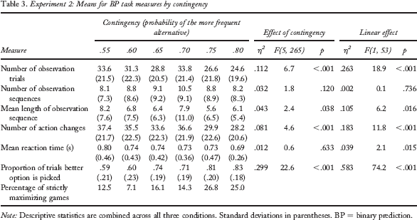
Note: Descriptive statistics are combined across all three conditions. Standard deviations in parentheses. BP = binary prediction.

The same set of dependent measures was analysed to examine the effect of game number (i.e., 1 = first, through 6 = last). With the exception of reaction time (see above), the effect of condition is small or small to medium and nonsignificant for all measures—all η_p² < 0.049, all F < 1.34, all p > .270—as is the case for the two-way interactions—all η_p² < 0.044, all F < 1.20, all p > .296. Thus, no clear differences in general patterns of responding were detected between the conditions, and no clear differential impacts of condition upon task experience were discerned. Whilst we cannot argue for the absence of any material effect of memory load from the absence of significant effects, we can say that we find little support for the conjecture that memory capacity is important because high-capacity participants retain free capacity for reasoning about the task whilst acquiring information. However, Table 4 does show a number of key effects of task experience upon data acquisition. There is a moderate decrease in the number of observations, most notably after the first game. This is the product of two very strong trends running in opposite directions. The number of observation sequences per game almost halves over the course of the experiment, whereas the number of observations per sequence roughly doubles. Participants seem to become more efficient in their data acquisition, which moves them towards the normative pattern of information acquisition prescribed for this task (collect all information in a single observation sequence). With respect to participants’ choices, there is an increase in the number of strictly maximizing participants over the course of the experiment: from around 10% in the first two games, to 25% in the last two. A Cochran's Q test confirmed that the proportion of strictly maximizing participants alters significantly over the 6 games, p = .001, and pairwise comparisons using McNemar's test show that strict maximization is significantly less common in Game 1 than in Games 4–6 and significantly less common in Game 3 than in Games 5–6. However, although the mean proportion of times that the better alternative is picked does fluctuate a little from game to game, η² = .040, F(5, 265) = 2.2, p = .053, there is no systematic increase in the proportion of times that the better alternative is picked (weak nonsignificant linear trend), η² = .019, F(1, 53) = 1.0, p = .317. This mean proportion is a little higher in the third game (.75) than in the first two (.67 in each), but this improvement is not sustained (.69 in Game 6). Similarly, mean winnings change little from one game to the next: effect of game, η² = .027, F(5, 265) = 1.5, p = .200. Thus it would appear that those participants who do not come to adopt the optimal (maximizing) strategy are not gradually becoming more optimal in their responding. In fact, analysis of the responding of the 35 participants who never maximized (in any game) shows that their mean proportion for the amount of times the better light is selected shows little consistent change: .62, .62, .66, .61, .68, and .61 across Games 1–6, respectively. The average level of responding with the better alternative for these participants shows slight undermatching (e.g., mean proportions of .53 and .57 when p = .55 and p = .60, but mean proportions of .72 and .74 for p = .75 and p = .80). In contrast, those who sometimes maximize increase from a mean proportion for the better alternative of .76 across Games 1–2 to a mean proportion of .86 across Games 3–6, and (unsurprisingly) they are on average overmatching to a considerable degree.

Table 4

Experiment 2: Mean for BP task measures by game number

Measure	Game number (1 = first, through 6 = last)						Effect of game			Linear effect
Measure	1	2	3	4	5	6	η²	F(5, 265)	p	η²	F(1, 53)	p
Number of observation trials	34.2 (22.9)	30.0 (20.6)	29.5 (22.6)	28.4 (20.5)	27.6 (21.1)	29.5 (20.6)	.043	2.4	.038	.079	4.6	.037
Number of observation sequences	13.6 (8.6)	10.1 (8.6)	7.9 (8.3)	8.0 (8.6)	6.6 (7.5)	8.1 (8.6)	.265	19.1	<.001	.376	31.9	<.001
Mean length of observation sequence	3.4 (3.8)	5.3 (5.5)	7.1 (6.9)	7.8 (8.1)	8.2 (8.1)	8.3 (10.0)	.153	9.5	<.001	.297	22.4	<.001
Number of action changes	42.3 (19.6)	37.5 (20.9)	31.4 (21.1)	33.4 (22.5)	26.6 (21.1)	31.9 (24.4)	.160	10.1	<.001	.338	27.1	<.001
Percentage of strictly maximizing games	5.4	12.5	12.5	19.6	25.0	25.0

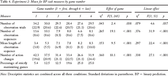
Note: Descriptive statistics are combined across all three conditions. Standard deviations in parentheses. BP = binary prediction.

The most commonly selected strategy for the die problem questionnaire was the matching strategy (pick according to the ratio of colours), which 22 (39%) of participants endorsed. A total of 14 (25%) selected the maximizing strategy, 12 (21%) selected Strategy B (mostly red), and 8 (14%) selected Strategy E (switch with runs). There is a clear alignment between endorsing maximization in the die problem and adopting an equivalent strategy in the BP task. For instance, of the 14 participants who picked the maximizing strategy in the die problem, 8 (57%) strictly maximized in the final BP game, whereas of the 42 who picked another die problem strategy, only 6 (14%) strictly maximized in the final BP game. Whilst not unexpected, this finding is important. Experimenters have noted that, in versions of the BP task where participants receive trial-by-trial feedback, participants may consciously adopt a matching strategy over a maximizing strategy that they know to be (financially) superior, as the “challenge” of predicting rare occurrences relieves the boredom of the task (Brackbill et al., 1962). In contrast, these data suggest that (perhaps because they had no feedback on their choices) participants mostly followed the strategy that they believed would maximize the financial pay-offs.

Table 5 shows the correlation between cognitive capacity and BP task measures. The degree of positive correlation between Raven's matrices and working memory capacity here (around r = .3) is similar to that found in other investigations (Engle et al., 1999; Mogle, Lovett, Stawski, & Sliwinski, 2008). Examining the measures related to information acquisition, the number of observation sequences (positively) predicts much more of the variance in the number of observation trials than the length of observation sequences does. And, perhaps predictably, participants making fewer observations tend to make markedly more observations within each sequence. Key for our purposes is the observation that higher cognitive capacity predicts both more optimal information acquisition (an effect that was not so evident in Experiment 1) and more optimal choice behaviour (which replicates what was observed in Experiment 1). This pattern is seen most clearly for Raven's matrices scores and is a little less clear for WM score and (a little less still) for digit span. Most of these key relationships represent small-to-medium and medium-sized effects (Cohen, 1992)—but the pattern of relationships is both coherent and regular for all three measures of cognitive capacity. Thus participants with higher cognitive capacity make longer sequences of observations (medium effect) within slightly fewer observation sequences (small effect) and make fewer action changes (small-to-medium effect). Thus, to some degree, information acquisition is less distributed (i.e., more optimal). Participants with higher Raven's matrices or WM scores select the better option and adopt the optimal maximizing strategy more often (small-to-medium effect) and earn higher winnings (medium effect). Also, higher cognitive capacity predicts marginally quicker responding. Thus, although some of these relationships are weak and not significant, when considered together a clear pattern emerges that (consistent with Experiment 1) cognitive capacity predicts more efficient and more effective responding. The final column of the correlation matrix shows the relationship between die problem strategy and cognitive capacity or BP performance (1 = maximizing, 0 = other strategy; hence positive coefficients denote higher mean values of the measure for those selecting the maximizing strategy). Consistent with Gal and Baron (1996), intelligence significantly predicts selection of the maximizing strategy. Crucially, explicit strategy endorsement in the die problem also aligns with more optimal BP task performance: more BP maximizing and selecting the better alternative more often (both very large effects). Moreover, die problem maximizers made fewer but longer observation sequences and fewer action changes (i.e., less distributed and therefore more optimal information acquisition) and responded slightly more quickly.

Table 5

Experiment 2: Correlations for cognitive capacity and BP task measures

	2. WM score	3. Raven's matrices	4. No. obs. trials	5. No. obs. sequences	6. Length obs. sequence	7. RT	8. No. action changes	9. Prop'n better alt've	10. No. BP max. strategy games	11. Winnings	12. Max. strategy on die problem
1. Digit span	.11	.09	−.11	−.19	.16	−.20	−.23	.13	−.00	.25⁺	.13
2. WM score		.36^**	.10	−.06	.31^*	−.07	−.18	.23	.27⁺	.18	.18
3. Raven's matrices score			−.00	−.09	.28^*	−.17	−.24	.25⁺	.18	.34^**	.28^*
4. Number of observation trials				.60^***	.09	−.06	−.01	.09	−.10	−.11	−.10
5. Number of observation sequences					−.51^***	.02	.61^***	−.22	−.38^**	−.29^*	−.26^*
6. Length of observation sequence						−.10	−.71^***	.55^***	.54^***	.47^***	.29^*
7. RT							.11	−.12	−.07	−.07	−.24⁺
8. Number of action changes								−.76^***	−.74^***	−.71^***	−.50^***
9. Proportion of times better alternative is picked									.76^***	.89^***	.57^***
10. Number of BP maximizing strategy games										.74	.63^***
11. Winnings for BP task											.55^***

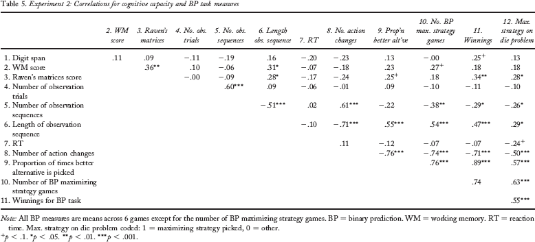
All BP measures are means across 6 games except for the number of BP maximizing strategy games. BP = binary prediction. WM = working memory. RT = reaction time. Max. strategy on die problem coded: 1 = maximizing strategy picked, 0 = other.

p < .1.

p < .05.

p < .01.

***

p < .001.

Key Findings from Experiment 2

Maximizing in the BP task increased with contingency (probability of the more frequent alternative) and with task practice (i.e., the number of games completed). The amount of information acquired decreased (appropriately) with increasing contingency, and the efficiency of information acquisition increased with task practice. Higher cognitive capacity predicted more efficient information acquisition, more successful choice behaviour in the BP task, and endorsement of the optimal strategy in the die problem. In the absence of a significant effect of memory load upon choice, there was no evidence that the advantage for superior cognitive capacity was due to “online” strategy change afforded by “spare” capacity.

General Discussion

Our introduction addressed two ways in which memory constraints might be important in the binary prediction task: first in relation to information acquisition, and second in relation to choice behaviour. We found that participants with greater cognitive capacity were more successful in their choice strategies and that they often acquired information in a different manner to participants with lower cognitive capacity. We begin this general discussion by examining the impact of memory constraints upon choice strategy and then consider the role of memory constraints in information acquisition and information use.

Memory and Choice in the BP Task

We found that high working memory capacity (and high IQ in Experiment 2) predicted a higher proportion of maximizing choices and more frequent use of a strict maximizing strategy. These results are consistent with West and Stanovich (2003) and Gal and Baron (1996) who found that higher cognitive ability (assessed by SAT scores, or inferred from age) was associated with selecting a maximizing strategy more often and a matching strategy less often in BP tasks. However, our findings are an important extension of earlier work, as we employed an “experience-based” BP task where information is acquired through trial-by-trial observation, whereas West and Stanovich (2003) and Gal and Baron (1996) used only “described” BP tasks where outcome probabilities were specified in advance.

Our findings are intriguing because, on first inspection, they seem to contradict some recent investigations using trial-by-trial BP tasks where behaviour closer to maximizing is associated with lower cognitive capacity. Using a task sharing important features with the BP task, Kareev et al. (1997) found more maximizing-type behaviour among participants with lower memory capacity—a finding that was confirmed, at least for initial responding (prior to changes in the probabilities for each option), by Gaissmaier et al. (2006) using a more standard BP task. Moreover, Wolford et al. (2004) found maximizing to be more common when participants undertook a BP task with a secondary load (something that we found to have no significant effect upon choice). However, it is important to note a key difference between the task employed in this paper and the task used in previous investigations. Unlike other versions of the BP task, participants in the observe-or-bet BP task (Tversky & Edwards, 1966) do not receive feedback on their predictions. This is important as Gaissmaier et al. (2006) and Wolford et al. (2004) interpret their results in terms of individuals with high cognitive capacity searching for complex patterns (see also Gaissmaier & Schooler, 2008). In contrast, low-capacity individuals adopt a simpler approach that may lead them to be more influenced by the majority outcome. The discrepancy between our results implies that feedback may be crucial to this process of pattern searching. Observation trials in the observe-or-bet BP task do allow participants to examine the environment for patterns. However, feedback would be required for explicit hypothesis testing about the existence of patterns. Thus it is possible to reconcile our results with those of Kareev et al. (1997), Gaissmaier et al. (2006), and Wolford et al. (2004) if one acknowledges that removing feedback makes it harder for participants to actively test for patterns, thereby encouraging those who would otherwise explore the possibility of complex patterns to put their effort into determining the best strategy for choice. This interpretation is consistent with recent research that has highlighted the discrepancy between active prediction and passive observation, and between repeated choice with feedback and without feedback (Newell & Rakow, 2007; Rakow, Demes, & Newell, 2008)

At several points in our discussion we have presented maximizing as a qualitatively different mode of decision making. A comparison of data acquisition between participants who sometimes maximized (“sometimes-maximizers”) and those who never maximized (“never-maximizers”) in the BP task supports this assertion. The amount of information acquired by never-maximizers varied little across contingencies (means ranging from 26.9 to 34.0). In contrast, the sometimes-maximizers made markedly fewer observations for higher contingencies: with means of 35.7 and 35.0 for p = .55 and .60, falling to means of 20.5 and 20.9 for p = .75 and .80. This linear trend for contingency was extremely large for the sometimes maximizers (η_p² = 0.500, in comparison to a η_p² of 0.125 for this linear trend among never-maximizers). This discrepancy is consistent with maximizing driving information acquisition. In order to maximize, it is sufficient to sample information until one is confident about which alternative is the more frequent of the two, something that can be achieved with fewer observations with more extreme contingencies (as instantiated in belief updating and threshold models of decision making—see Busemeyer & Townsend, 1993; March, 1996; Sarin & Vahid, 2001). In contrast, if one's goal is to match there is no reason to alter data acquisition with contingency—and indeed, the never-maximizers sample a fairly constant amount of information. Moreover, never-maximizers are much more likely than sometimes-maximizers to make short sequences of observations (often just one or two at a time). For instance, averaging across contingencies, 85% of never-maximizers have a mean length of observation sequence below 7, whereas this is true for only 47% of the sometimes-maximizers. Again, it should not surprise us that the simple task of tallying observations to determine the more frequent of two outcomes is conducive to collecting more information in a single sequence.

Binary Prediction and the Narrow Window of Immediate Memory

Our introduction posed the question of whether Kareev's narrow window hypothesis of information use might have heuristic value in making predictions concerning information acquisition (Kareev, 1995a, 1995b, 2000; Kareev et al., 1997). With respect to the most straightforward prediction that could be made, the answer is a tentative “yes”: Participants with greater memory capacity tended to make more observations in a given sequence of observations. This relationship was not strong but was nontrivial (r ≈ .2 in Experiment 1, and r ≈ .3 in Experiment 2) and was similar to that observed between WM score and the amount of predecisional information that participants examined prior to making one-shot decisions in a decisions-from-sampling experiment (Rakow et al., 2008). However, the narrow window defined by traditional estimates of WM capacity does not act as a strict upper limit for the amount of information that participants were willing to observe in a single sequence. Short bursts of observations were the norm (e.g., mean lengths of observation sequences were around 7±2)—but individual sequences of 10 to 20 observations were not uncommon for some individuals. Thus, whilst individual differences in WM capacity predict variation in information acquisition, the “narrow window” of working memory does not provide a strict limit for data acquisition.

However, closer examination of our data implies that the narrow window hypothesis can offer some key insights into our choice data. In order to illustrate this, we consider three questions: (a) How were participants’ predictions distributed? (b) What outcomes did participants see when observing? (c) What outcomes would they see if observing/recalling through a narrow window?

Figure 1 shows the distribution of choices (the proportion of times that the better alternative is chosen) for each of the six contingencies that we examined (Experiment 2). The most remarkable feature of these distributions is just how rare matching is. Matching was the modal strategy selected in the die problem, and many participants described aiming for matching-type strategies when debriefed. Yet, for a contingency of p = .55, not a single participant chose the more frequent alternative with probability .55±.025, and only a handful of participants managed to match the contingency to within ±.025 in the other BP games. One can see that the means of these distributions (which alternate between overmatching and matching in the aggregate) are the product of the proportions generated by a minority of participants who maximize or near maximize and the proportions of a larger number of participants who seemingly do a wide range of things (but only very few of whom can be said to “match”).

Figure 1.

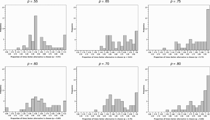
Distribution for the proportion of times the better alternative was chosen, for each contingency (Experiment 2).

However, it may be too hasty to assume that matching in BP prediction is simply an artefact of averaging. You will recall that participants in the observe-or-bet task only observe outcomes for a subset of trials (mean sample size around 30 out the 100 trials, but with considerable variance in sample size). Thus whilst sampling theory predicts that the mean number of times that the better alternative is seen will be close to the programmed contingency, some individual participants experience higher proportions whilst others experience a proportion that is below the programmed contingency. Figure 2 shows what participants actually saw when the probability of the better alternative was .60, .70, or .80 (other contingencies are omitted to conserve space and avoid redundancy). Participants did indeed experience a range of probabilities—but, as befits a typical sample size of 30, the proportion of times that the better alternative was observed was usually relatively close to its “true” probability (at least for p = .70 or .80). Whatever qualitative judgement one makes concerning “how close is close?”, one thing that is clear from comparing Figures 1 and 2 is that the distributions for choices is much wider than the distributions for what was observed. This remains the case even if one takes the maximizers out of the picture (on the basis that they were not seeking to match and were engaged in qualitatively different behaviour—see above). To put it another way, if most participants simply matched what they had observed when making predictions, the distribution of responses in Figure 1 would show a much sharper peak lying close to the programmed probability for the better alternative. Thus, sampling variability in what participants observed does not explain the rarity of actual matching behaviour.

Figure 2.

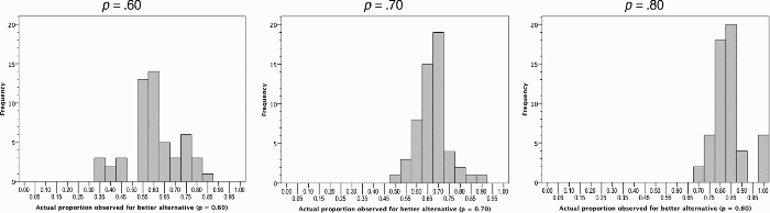
Distributions for the actual proportion of times that the better alternative was observed by participants (Experiment 2).

How might this discrepancy be explained? One consideration is that many participants distributed their observations. Thus, some predictions were made without the benefit of the full set of observations represented in Figure 2. For instance, a participant seeking to make a series matching predictions on the basis of an initial 10 observations would have less chance of closely matching the true probability than when making a later set of predictions on the basis of 30 observations. That said, if participants simply followed each sequence of observations with a matched set of predictions, they would closely match the observed probability. (Matching would not be guaranteed perfect, as termination of the game could prevent or truncate or a final sequence of predictions.) More importantly (appealing to the role of representativeness in the conception of randomness, Kahneman & Tversky, 1972), a participant who believes that the sequence is random may believe that prediction according to repeated sequences is inappropriate, preferring to “simulate” a random sequence with the correct proportions. A similar logic would hold if a participant believes the sequence to be nonrandom, but too complex to identify repeated patterns.

So it is clear that participants do not consistently imitate what they observe (otherwise, Figures 1 and 2 would show greater similarity), and the previous paragraph identifies some reasons why this should be so. However, imagine that, as Kareev suggests, participants recall a small sample of observations, for instance, around five, seven, or nine depending upon their working memory capacity. Figure 3 illustrates this with two sets of examples, showing the expected distribution of outcomes for the better alternative. The upper row assumes that windows of size 5, 6, 7, 8, and 9 are all equally likely (i.e., Miller's 7±2). The lower row assumes that all sizes of window from 5 to 11 are equally likely.² We modelled a range of window sizes as the presence of individual differences in WM capacity makes it unreasonable to assume a single size for all participants. The similarity of the two sets of distribution suggest that assumptions about the precise size of the small window are not particularly crucial, and, within reason, the particular distribution of window sizes is unlikely to make a large difference (Dawes, 1982; Dawes & Corrigan, 1974). Whilst by no means a perfect fit to the data shown in Figure 1 (even when a proportion of the maximizers are discounted), Figure 3 does illustrate how a “narrow window of experience” can account for the greater variance in response proportions (Figure 1) when compared to the observed proportions (Figure 2). Figure 3 also illustrates why there may be multiple modes to the distribution of response proportions that do not fall at the programmed probability even though the mean is close to the programmed probability. Distributions based on small samples are “lumpy”: For instance, because proportions around .8 can be generated in multiple ways (e.g., 4/5, 7/9, 8/10) a peak may occur there even if this is not the mean of the distribution. It also illustrates how someone seeking to match may actually maximize on occasion, as small samples sometimes yield the same outcome (recall that participants who failed to identify maximizing as the optimal strategy in the die problem did occasionally maximize in the BP task).

We undertook an analysis of the size of window that provided a best fit to the standard deviations of the distributions shown in Figure 1, testing windows up to n = 13: This analysis excluded participants who strictly maximized (on the basis that their behaviour was qualitatively distinct): (a) on a game-by-game basis, and (b) excluding participants who maximized on at least one game. Best fitting windows ranged from 5 to 11 depending upon the condition in Analysis a and ranged from 5 to 13+ in Analysis b. The median window size was 8 over both analyses, and it is on this basis that we provide our second set of distributions based on windows of size 8±3.

Figure 3.

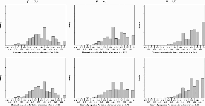
Distributions for the expected proportion of times the better alternative is observed, assuming windows of size (a) 7±2 (upper row), and (b) 8±3 (lower row).

We are unable to determine from our data whether the narrow window hypothesis should be taken as a literal process model. All that can be said is that it is as if the data acquired are viewed through a narrow window, which is equivalent to saying that only some of the available information is effectively utilized. For instance, it may be that a narrow window limits the output of responses rather than limiting the recall of information—and so predictions could be based on fine-grained beliefs about event probabilities, but are output as pseudorandom sequences of left–right predictions of length around 7±2.

In conclusion, our data point to heuristic value for the narrow window hypothesis of information sampling—though, unlike for other variants of the BP task (Kareev et al., 1997; Wolford et al., 2004), a narrow window (as determined by WM capacity) confers no advantage (see Anderson et al., 2005; Juslin & Olsson, 2005). In fact, higher cognitive capacity predicted better task performance. Our interpretation is that this version of the BP task (which separates out information acquisition from choice) encourages higher capacity individuals towards successful identification of the optimal choice strategy. This then moves these participants towards more efficient information acquisition.

Footnotes

Appendix

References

Anderson

R. B.

Doherty

M. E.

Berg

N. D.

Friedrich

J. C.

(2005). Sample size and the detection of correlation—a signal detection account: Comment on Kareev (2000) and Juslin and Olsson. Psychological Review 112, 268–279.

Bereby-Meyer

Erev

(1998). On learning to become a successful loser: A comparison of alternative abstractions of learning processes in the loss domain. Journal of Mathematical Psychology 42, 266–286.

Brackbill

Kappy

M. S.

Starr

R. H.

(1962). Magnitude of reward and probability learning. Journal of Experimental Psychology 63, 32–35.

Busemeyer

J. R.

Townsend

J. T.

(1993). Decision field theory: A dynamic-cognitive approach to decision making in an uncertain environment. Psychological Review 100, 432–459.

Cohen

(1992). A power primer. Psychological Bulletin 112, 155–159.

Conway

A. R. A.

Kane

M. J.

Bunting

M. F.

Hambrick

D. Z.

Wilhelm

Engle

R. W.

(2005). Working memory span tasks: A methodological review and user's guide. Psychonomic Bulletin & Review 12, 769–786.

Daneman

Merikle

P. M.

(1996). Working memory and language comprehension: A meta-analysis. Psychonomic Bulletin and Review 3, 422–433.

Dawes

R. M.

(1982). The robust beauty of improper linear models. Kahneman

Slovic

Tversky

Judgment under uncertainty: Heuristics and biases. Cambridge, UK: Cambridge University Press 391–407.

Dawes

R. M.

Corrigan

(1974). Linear models in decision making. Psychological Bulletin 81, 95–106.

10.

Derks

P. L.

Paclisanu

M. I.

(1967). Simple strategies in binary prediction by children and adults. Journal of Experimental Psychology 73, 278–285.

11.

Dierckx

Vandierendonck

(2005). Adaptive strategy application in linear reasoning. Roberts

M. J.

Newton

E. J.

Methods of thought: Individual differences in reasoning strategies. Hove, UK: Psychology Press 107–127.

12.

Edwards

(1965). Optimal strategies for seeking information. Journal of Mathematical Psychology 2, 312–329.

13.

Elwin

Juslin

Olsson

Enkvist

(2007). Constructivist coding: Learning from selective feedback. Psychological Science 18, 105–110.

14.

Engle

R. W.

Nations

J. K.

Cantor

(1990). Is “working memory capacity” just another name for word knowledge. Journal of Educational Psychology 82, 799–804.

15.

Engle

R. W.

Tuholski

S. W.

Laughlin

J. E.

Conway

A. R. A.

(1999). Working memory, short-term memory, and general fluid intelligence: A latent variable approach. Journal of Experimental Psychology: General 128, 309–331.

16.

Fantino

Esfandiari

(2002). Probability matching: Encouraging optimal responding in humans. Canadian Journal of Experimental Psychology 56, 58–63.

17.

Gaissmaier

Schooler

L. J.

(2008). The smart potential behind probability matching. Cognition 109, 416–422.

18.

Gaissmaier

Schooler

L. J.

Rieskamp

(2006). Simple predictions fueled by capacity limitations: When are they successful?. Journal of Experimental Psychology: Learning, Memory and Cognition 32, 966–982.

19.

Gal

Baron

(1996). Understanding repeated simple choices. Thinking and Reasoning 2, 81–98.

20.

Goodnow

J. J.

(1955). Determinants of choice-distribution in two-choice situations. American Journal of Psychology 68, 106–116.

21.

Hitch

G. J.

Halliday

M. S.

Littler

J. E.

(1989). Item identification time and rehearsal as predictors of memory span in children. Quarterly Journal of Experimental Psychology 82, 375–386.

22.

Hogarth

R. M.

(2006). Is confidence in decisions related to feedback? Evidence from random samples of real-world behavior. Fiedler

Juslin

Information sampling and adaptive cognition. Cambridge, UK: Cambridge University Press 456–484.

23.

Humphreys

L. G.

(1939). Acquisition and extinction of verbal expectations in a situation analogous to conditioning. Journal of Experimental Psychology 25, 294–301.

24.

Juslin

Olsson

(2005). Capacity limitations and the detection of correlations: Comment on Kareev (2000). Psychological Review 112, 256–267.

25.

Kahneman

Tversky

(1972). Subjective probability: A judgment of representativeness. Cognitive Psychology 3, 430–454.

26.

Kareev

(1995a). Positive bias in the perception of covariation. Psychological Review 102, 490–502.

27.

Kareev

(1995b). Through a narrow window: Working memory capacity and the detection of covariation. Cognition 56, 263–269.

28.

Kareev

(2000). Seven (indeed, plus or minus two) and the detection of correlations. Psychological Review 107, 397–402.

29.

Kareev

(2005). And yet the small-sample effect does hold: Reply to Juslin and Olsson (2005) and Anderson, Doherty, Berg, and Friedrich (2005). Psychological Review 112, 280–285.

30.

Kareev

Lieberman

Lev

(1997). Through a narrow window: Sample size and the perception of correlation. Journal of Experimental Psychology: General 126, 278–287.

31.

Kyllonen

P. C.

(1996). Is working memory capacity Spearman's g?. Dennis

Tapsfield

Human abilities: Their nature and measurement. Mahwah, NJ: Lawrence Erlbaum Associates 49–76.

32.

March

J. G.

(1996). Learning to be risk averse. Psychological Review 103, 309–319.

33.

Meo

Roberts

M. J.

Marucci

F. S.

(2007). Element salience as a predictor of item difficulty for Raven's Progressive Matrices. Intelligence 35, 359–368.

34.

Miller

G. A.

(1956). The magical number seven, plus or minus two: Some limits on our capacity for processing information. Psychological Review 63, 81–97.

35.

Mogle

J. A.

Lovett

B. J.

Stawski

R. S.

Sliwinski

M. J.

(2008). What's so special about working memory? An examination of the realtionship among working memory, secondary memory, and fluid intelligence. Psychological Science 19, 1071–1077.

36.

Newell

B. R.

Rakow

(2007). The role of experience in decisions from description. Psychonomic Bulletin and Review 14, 1133–1139.

37.

Nies

R. C.

(1962). Effects of probable outcome information on two-choice learning. Journal of Experimental Psychology 64, 430–433.

38.

Peterson

C. R.

Ulehla

Z. J.

(1965). Sequential patterns and maximizing. Journal of Experimental Psychology 69, 1–4.

39.

Rakow

Demes

K. A.

Newell

B. R.

(2008). Biased samples not mode of presentation: Re-examining the apparent underweighting of rare events in experience-based choice. Organizational Behavior and Human Decision Processes 106, 168–179.

40.

Sarin

Vahid

(2001). Predicting how people play games: A simple dynamic model of choice. Games and Economic Behavior 34, 104–122.

41.

Stanovich

K. E.

West

R. F.

(2000). Individual differences in reasoning: Implications for the rationality debate?. Behavioral and Brain Sciences 23, 645–726.

42.

Turner

M. L.

Engle

R. W.

(1989). Is working memory capacity task dependent?. Journal of Memory and Language 28, 127–154.

43.

Tversky

Edwards

(1966). Information versus reward in binary choices. Journal of Experimental Psychology 71, 680–683.

44.

Wechsler

(1997). Wechsler Memory Scale–Third Edition San Antonio, TX: The Psychological Corporation.

45.

West

R. F.

Stanovich

K. E.

(2003). Is probability matching smart? Associations between probabilistic choices and cognitive ability. Memory and Cognition 31, 243–251.

46.

Wolford

Newman

S. E.

Miller

M. B.

Wig

G. S.

(2004). Searching for patterns in random sequences. Canadian Journal of Experimental Psychology 58, 221–228.