Human instrumental performance in ratio and interval contingencies: A challenge for associative theory

Abstract

Associative learning theories regard the probability of reinforcement as the critical factor determining responding. However, the role of this factor in instrumental conditioning is not completely clear. In fact, free-operant experiments show that participants respond at a higher rate on variable ratio than on variable interval schedules even though the reinforcement probability is matched between the schedules. This difference has been attributed to the differential reinforcement of long inter-response times (IRTs) by interval schedules, which acts to slow responding. In the present study, we used a novel experimental design to investigate human responding under random ratio (RR) and regulated probability interval (RPI) schedules, a type of interval schedule that sets a reinforcement probability independently of the IRT duration. Participants responded on each type of schedule before a final choice test in which they distributed responding between two schedules similar to those experienced during training. Although response rates did not differ during training, the participants responded at a lower rate on the RPI schedule than on the matched RR schedule during the choice test. This preference cannot be attributed to a higher probability of reinforcement for long IRTs and questions the idea that similar associative processes underlie classical and instrumental conditioning.

Keywords

Associative theories Causal learning Goal-directed behaviour Habits Instrumental learning Reinforcement schedules

In both his learning texts, The Psychology of Animal Learning (1974) and Conditioning and Associative Learning (1983), Nicholas Mackintosh argues that common associative learning processes underlie Pavlovian and instrumental conditioning on the basis of the empirical commonalties between the different forms of learning. For example, in a series of experiments, Wagner demonstrated that when a target cue is trained in compound with another stimulus, the amount of conditioning accruing to the target depends upon its validity as a predictor of the reinforcer relative to the other stimulus (Wagner, 1969; Wagner, Logan, & Haberlandt, 1968). Mackintosh then notes that instrumental conditioning of wheel running shows comparable sensitivity to the relative validity of this response as a predictor of a food reinforcer (Mackintosh & Dickinson, 1979).

The effect of relative validity in Pavlovian conditioning is most readily explained by associative theories that deploy a prediction error to modulate learning (Mackintosh, 1975; Rescorla & Wagner, 1972; for a review, see Vogel, Castro, & Saavedra, 2004). At the core of all such theories is the claim that the net associative strength of a stimulus normally increases when it is paired with a reinforcer and normally decreases when it is presented in the absence of the reinforcer. As a consequence, a primary determinant of conditioning is the probability of reinforcement, a factor that raises a potential problem for the application of such associative theories to instrumental conditioning.

The problem arises from the contrast between different schedules of instrumental reinforcement. On variable ratio (VR) schedules, reinforcers are delivered after the agent performs a certain number of responses, whereas on variable interval (VI) schedules these are delivered for the first response made after a certain period of time has elapsed since the last reinforcer. The required interval or number of responses vary after each reinforcement around a pre-determined average. For example, a VR10 schedule will return a reinforcer, on average, after every 10 responses; a VI10 schedule will reward the first response made after, on average, 10 s since the last reinforced response. These schedules are thought to model, respectively, the non-depleting and depleting and regenerating resources that animals may find in their natural environments (Dickinson, 1994). The idealized versions of these two schedules are the random ratio (RR) and random interval (RI) schedules, where the probability of reinforcement per response—in the ratio case—and the probability of a reinforcer becoming available per second—in the interval case—are given by binomial (or geometric) distribution (see Cardinal & Aitken, 2010). Using a variety of species and target instrumental responses, a wealth of evidence has shown that ratio schedules support higher response rates than interval schedules despite the probability of reinforcement or the reinforcement rate being matched (Bradshaw, Freegard, & Reed, 2015; Bradshaw & Reed, 2012; Catania, Matthews, Silverman, & Yohalem, 1977; Dawson & Dickinson, 1990; Peele, Casey, & Silberberg, 1984; Reed, 2001a, 2001c; Zuriff, 1970).

Mackintosh (1974) was fully aware of the ratio–interval contrast and discussed whether ratio and interval schedules differentially reinforce divergent response rates—that is, whether different response rates bring about different reinforcement probabilities on ratio and interval schedules. While dismissing the misconception that VR schedules differentially reinforce high rates of responding, he notes that, unlike ratio schedules, interval schedules differentially reinforce long inter-response times (IRTs), or the pause between responses. On an interval schedule, the longer that an agent waits before responding again, the more likely it is that a reward will have become available. This contingency implies that long IRTs will be correlated with higher probabilities of reinforcement for the next response. Because the reinforcement probability on VR schedules does not vary with IRT size, it follows that agents should emit longer IRTs, or pauses between responses, on VI schedules and therefore respond less often than on a VR schedule. Thus, by focusing on the temporal control of responding under interval contingencies, Mackintosh’s argument retains the probability of reinforcement as the cardinal determinant of responding.

Kuch and Platt (1976) proposed a schedule for evaluating the role of the differential reinforcement of long IRTs while retaining the relative independence of response rates and reinforcement rates characteristic of interval schedules. The regulated probability interval (RPI) schedule sets a probability of reinforcement for each response that will generate an average inter-reinforcement interval that matches the schedule parameter if the agent continues to respond at the current rate. This regulated probability is calculated as P = t/Tm, where t denotes the time it took the subject to perform the last m responses, and T is the scheduled inter-reinforcement interval. The equation can be also written as P = 1/Tb_m, where b^m can be regarded as the local response rate during the memory size m. Therefore, if the agent decreases b^m from a particular level, the probability of reinforcement will adjust—increasing in this case—so that the reward is delivered on average after a pre-set interval, thereby keeping the reinforcement rate constant at 1/T rewards per second. Suppose, for example, that m = 10, and the interval between reinforcers that the experimenter aims to achieve is 10 s (T = 10). Moreover, assume that the participant has performed 20 responses in the last 10 s, so that t = 5. Then the reinforcement probability for the next response will be 5/(10 × 10) = .05; at this rate, one every 20 responses on average will be rewarded. Because, on average, it takes the subject 10 s to perform 20 responses, then with a reinforcement probability of one in 20 (.05) the average interval between reinforcers will be 10 s. Suppose now that the agent responds less vigorously, so that it took 10 s to perform the last 10 responses (t = 10). Then the reinforcement probability will be 10/(10 × 10) = .1; at this new rate, 1 out of 10 responses on average will be rewarded. Since it takes the agent 10 s to perform them, the interval between reinforcers will be again 10 s.

The previous example shows that, in contrast with RI schedules, in the RPI schedule the reinforcement probability is fixed prior to the emission of a response so that it does not vary with the duration of the preceding IRT, but rather depends on a set of IRTs given by the memory size m. As a result, the RPI prevents the differential reinforcement of any particular IRT size while maintaining the pre-set average inter-reinforcement interval. Thus, if probabilities of reinforcement are matched, associative theories predict similar levels of responding for VR and RPI schedules.

Only a few studies have investigated the VR-RPI contrast. Dawson and Dickinson (1990) compared responding on VR, VI, and RPI schedules with triads of rats when the reinforcement rate of the interval schedules was matched to that generated by the ratio schedule by yoking within each triad. The fact that the rats responded more slowly on the VI than on the RPI schedule suggests that the differential reinforcement of long IRTs does slow responding under an interval contingency, whereas the higher response rate on the VR than on the RPI schedule indicates that this factor cannot be the sole cause of the ratio–interval difference. More recently, Tanno and Sakagami (2008) observed similar response rates when rats responded on VR and RPI schedules. However, in a further study with human participants, Tanno (2008) replicated the ordering of response rates observed by Dawson and Dickinson (1990)—although the critical contrast between the VR and RPI performance did not reach the standard criterion of statistical significance. Given the theoretical importance of this contrast, we re-examined human instrumental performance on VR and RPI schedules.

To this end, we matched the probability of reinforcement across RPI and RR schedules by yoking the value generated by performance on a master RPI schedule to that programmed by the RR contingency on both a within-participant and a between-participant basis. In addition, we trained some of the participants on an RPI schedule that programmed an average inter-reinforcement interval that matched the interval generated by their prior performance on an RR schedule. Following this training on the single RPI and RR schedules, we gave a choice between responding on the two types of schedules. If, as anticipated by associative theories, the probability of reinforcement is the primary determinant of responding, the participants should have responded at similar rates on the RR as on the RPI schedule in this choice test.

Experimental study

Method

Participants

Forty-five undergraduates from the University of Cambridge, who were naïve to the experimental procedure, participated in the experiment and gave informed consent. They were randomly assigned to one of four groups and were paid £3 plus a chocolate bar for their participation.

Apparatus

Participants were tested individually inside one of two testing rooms and were presented with the task on a laptop (15.4″ Acer Aspire 5930 or 15.4″ Asus K52J) running Windows 7. The experiment was programmed using Microsoft Visual Studio 2008. To prevent participants from being distracted by outside noise, all of them were asked to wear headphones during the task.

Design

There were four groups and two stages: training followed by the choice tests. As represented in the rows of Table 1, training started with a sequence of four 3-min trials in each of which responding was reinforced on a different schedule. For Group A1, training started with the master RPI 30-s schedule followed by training in the second trial on a yoked RR schedule, designated as a RRy30 schedule. For each participant, the mean probability of reinforcement generated by performance on the RPI 30-s schedule was used as the parameter for the RRy30, thereby yielding within-participant yoking of reinforcement probability. The next two training trials recapitulated this sequence with an RPI 10-s master schedule. This sequence was then repeated to generate a total of eight trials so that each schedule received a total of 6 min of training. The purpose of training on the RPI 10-s schedule was to yield a yoked RRy10 schedule with a higher reinforcement probability than that for the yoked RRy30 so that we could verify that performance on our task was sensitive to this well-established determinant of instrumental responding. To this end, the first 3-min choice test trial offered a choice between responding on the RRy10 and RRy30 schedules. If performance on this task is sensitive to reinforcement probability, the RRy10 schedule should have attracted more responding. Finally, the critical test offered a choice between the RPI 30-s and RRy30 schedules for participants in A1 or A2 groups.

Table 1.

Design of the experiment.

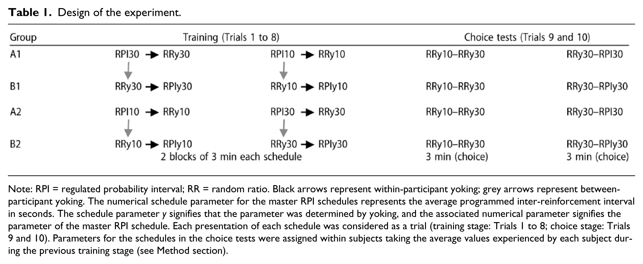
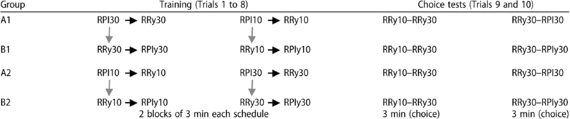
Note: RPI = regulated probability interval; RR = random ratio. Black arrows represent within-participant yoking; grey arrows represent between-participant yoking. The numerical schedule parameter for the master RPI schedules represents the average programmed inter-reinforcement interval in seconds. The schedule parameter y signifies that the parameter was determined by yoking, and the associated numerical parameter signifies the parameter of the master RPI schedule. Each presentation of each schedule was considered as a trial (training stage: Trials 1 to 8; choice stage: Trials 9 and 10). Parameters for the schedules in the choice tests were assigned within subjects taking the average values experienced by each subject during the previous training stage (see Method section).

Each participant in Group B1 was paired with a master participant in Group A1 so that, through between-participant yoking, the performance of the master on the RPI 30-s schedule set the probability of reinforcement scheduled by the initial RRy30 schedule received by the yoked B1 participant. This participant was then trained on an RPIy30 schedule for which the parameter was the mean inter-reinforcement interval generated by her prior performance on the RRy30 schedule. The next two trials recapitulated this yoking procedure for the 10-s parameter. The two choice test trials were the same as those for Group A1 except that the final trial gave a choice between the RRy30 and RPIy30 schedules.

Finally, Groups A2 and B2 received the same training and testing as did Groups A1 and B1, respectively, except for the fact their participants were initially trained on the master RPI 10-s schedule and the associated yoked schedules so that the order of training was counterbalanced across groups.

Procedure

The scenario required as the response the insertion of coin icons into dispensers in order to obtain M&M sweets as the reinforcer or outcome. Each schedule was associated with a different dispenser. Following the procedure used in similar studies (Bradshaw et al., 2015; Bradshaw & Reed, 2012; Reed, 2001c), the participants were given written instructions with the following text below:

During your time today you will be using coins to invest into M&Ms dispensers. You will have the opportunity to use your coins in different M&Ms dispensers, but only one of them will be turned on at each time. At any time you may invest a coin on a dispenser by pressing the spacebar. If you receive a return on your coins, then you will get one M&Ms bag. The total number of candies you have won and your total coin credit will be displayed on the top of the screen so you can monitor your performance.

Your aim is to make the most profits, i.e., to get the most M&Ms with the fewest coins. In doing so, you will need to use your coins the best way you can. Due to the nature of the dispenser machines it is to your advantage to insert coins some of the time and not to insert coins at other times. You need to discover this by yourself.

You will be shown 4 dispenser machines, only one of which is active at a time. You have to select the active machine by clicking on it. To indicate that the machine is active, a hand holding a coin will be shown above the selected machine. To insert a coin in the active machine, press the spacebar. You may insert coins at any time. Every time a coin earns you a reward (M&Ms candy), you have to collect it by clicking on the “collect” image that will appear on the screen and then select the machine again to be able to insert coins again. The following screenshot explains the display you will see: (a screenshot of the task was presented)

Your performance will be recorded and ranked among the performance of other participants; the 3 participants who used their coins most efficiently (i.e., highest number of M&Ms collected with the fewest coins) will receive special rewards.

After it had been checked that participants understood the instructions, they started responding on the first training schedules assigned to their group, as outlined in the Design section. Four M&M dispensers were aligned in the lower part of the screen from left to right (see Figure 1). The combination of the image of each machine and the position was randomized between subjects. The active schedule was signalled by a hand holding a coin on top of the dispenser; a banner in front of the other machines with the phrase “not in use” signalled that the other schedules were inactive. Upon completion of 3 min of training on the first schedule, the next schedule was activated, and the hand moved to its corresponding position. The banner now appeared in front of the previous dispenser. This process continued until the eight trials were completed.

Figure 1.

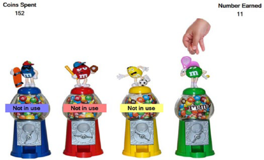
A screenshot of the task as seen by participants. To view this figure in colour, please visit the online version of this Journal.

In the upper part of the screen, the number of M&Ms obtained in the task and the number of coins spent were shown in the upper corners. In contrast to the majority of human studies using free-operant schedules (Bradshaw et al., 2015; Bradshaw & Reed, 2012; McDowell & Wixted, 1986; Reed, 2001a, 2001b, 2001c), participants were not shown the number of credits remaining, but only the total number they had so far spent during the task. This display informed participants the overall number of responses performed, but no information about current performance was provided. Based on a previous pilot study, we thought that this procedure would encourage participants to maintain responding and not to consider stopping as a strategy for maximizing the amount of credits obtained in the task.

We also added a collection procedure. To collect the M&M, participants were asked to click on the upper part of the screen where an image of an M&M bag appeared. They then had to return to the dispenser and click on it in order to activate it and start responding again. Every time a reward occurred, the timer for the task was paused and re-started only after the participant clicked on the M&M bag. The addition of this “consummatory” response was based on previous data suggesting that, under certain conditions, this response might be necessary for human participants to show performance similar to that observed in non-human animals (Bradshaw & Reed, 2012; Reed, 2007a).

The choice test started immediately after training finished (see Table 1). Two different dispensers were active at the same time, and, in order to insert coins, participants had to choose one of the dispensers by clicking on it. The hand holding the coin appeared on top of the dispenser every time the choice occurred.

Both RR and RPI schedules specified the probability that each insertion of a coin into a dispenser would yield M&Ms. In the case of the RR schedule, the reinforcement probability was simply the reciprocal of the schedule parameter, which was determined for each participant and schedule by the yoking procedure. If, for example, the yoking procedure led to an RR schedule delivering reinforcement after five responses on average, then reinforcement probability was simply 1/5. The probability of a response being rewarded on a RPI schedule was t/Tm, where the schedule parameter T was the programmed mean inter-reinforcement interval that the schedule aimed to maintain, and t was the total duration of the last m IRTs which, when divided by m, represented the mean IRT during this period, or the local rate of responding. Therefore, on the RPI schedule, the probability that a particular response was reinforced did not depend on the last IRT, but on a set of m IRTs. As Dawson and Dickinson (1990) found that the performance of their rats was unaffected by the value of m when varied between 1, 5, and 50, we assigned a value of 5 to m. The algorithm for the regulated probability was set so that if the number of responses was less than the memory size of 5, the probability of reinforcement for the next response was calculated by taking the response rate for the number of responses currently emitted since the beginning of the trial. After five responses were emitted, the regulated probability was calculated with the memory size of 5 for the rest of the trial.

Results

Nine participants in total were discarded from the analysis either because they failed to respond in at least one of the master schedules, thereby producing undefined parameters for the yoked schedules, or because response rates for at least one master RPI schedule were so high that probabilities of reinforcement for the yoked participant were less than .02, which would not allow the yoked participant to experience the schedule contingency during a 3-min trial. Participants that did not meet the criteria were excluded immediately after testing by examining their performance and before testing the next participant. This resulted in the following number of participants excluded from each group: Group A1: two participants; Group B1: two participants; Group A2: four participants; Group B2: one participant. Following these exclusions, each group consisted of nine participants.

Choice test

As shown in Figure 2, participants responded at a higher rate on the RRy10 schedule than on the RRy30, F(1, 34) = 21.01, p < .01, η² = .38, 90% confidence interval, CI [.17, .53], thereby confirming that performance in this choice test is sensitive to a major determinant of instrumental responding, the reinforcement probability. Of most theoretical significance, however, is the finding that the RRy30 schedule attracted a higher rate of responding than the RPI30/y30 schedules, F(1, 34) = 5.53, p=.02, η² = .14, 90% CI [.01, .31], despite the reinforcement probabilities being the same. The magnitudes of these schedules effects did not vary reliable across the four groups. There was no significant effect of group on the response rate nor a significant Schedule × Group interaction for the RRy10–RRy30 contrast—F(1, 34) = 0.26, p = .61, η² = .01, 90% CI [.00, .11]; F(3, 34) = 0.91, p = .35, η² = .07, 90% CI [.00, .18], respectively—and the RRy30–RPI30/y30 contrast—F(1, 34) = 0.29, p = .60, η² = .01, 90% CI [.00, .11]; F(3, 34) = 1.15, p = .29, η² = .09, 90% CI [.00, .20], respectively.

Figure 2.

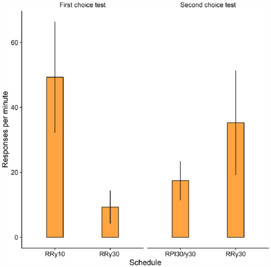
Mean response rates in the two choice tests (Trials 9 and 10). RPI = regulated probability interval; RR = random ratio. Error bars indicate 95% confidence intervals.

Training

Table 2 shows that the response rates were uniformly high during the last four trials of training (the second 3-min trials for each schedule). The effects of schedule, F(3, 102) = 0.28, p = .84, η² = .01, 90% CI [.00, .03], and group, F(1, 34) = 1.06, p = .31, η² = .03, 90% CI [.00, .17]), and their interaction, F(3, 102) = 0.60, p = .62, η² = .02, 90% CI [.00, .05], were not significant. We suspect that the effects of these factors, which were evident during the choice test, were not observed in training because the low cost of responding did not constrain performance in the way that the choice of one option at test constrained performance on the other option.

Table 2.

Mean values and 95% CIs for response rates, ratio of mean reinforced IRT to mean overall IRT, and probability of reinforcement for RR and RPI schedules during the final four trials of training.

Schedule	Response rate		IRT ratio		Probability of reinforcement
Schedule	M	CI	M	CI	M	CI
RPI10/y10	48.8	[32.0, 65.6]	1.2	[1.0, 1.5]	.17	[.12, .21]
RPI30/y30	48.9	[26.7, 71.0]	1.3	[0.8, 1.7]	.08	[.05, .10]
RRy10	48.5	[33.8, 63.2]	1.0	[0.9, 1.1]	.23	[.17, .28]
RRy30	54.4	[33.1, 75.6]	1.0	[0.7, 1.2]	.08	[.05, .12]

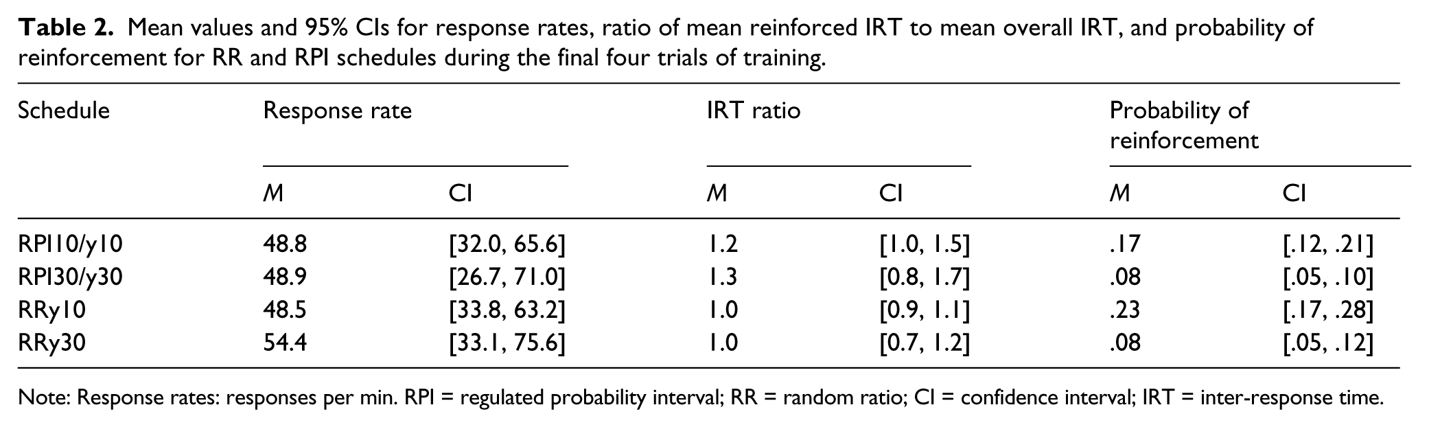
Note: Response rates: responses per min. RPI = regulated probability interval; RR = random ratio; CI = confidence interval; IRT = inter-response time.

Yoking analysis

As noted in the introduction, the reason for using the RPI schedule to examine the ratio–interval contrast is the fact that this schedule controls the differential reinforcement of long IRTs produced by standard interval schedules. Therefore, if our yoking procedure was successful in controlling for reinforcement probability, then associative theories predict similar levels of responding for RR and RPI schedules in the choice test. To investigate whether these conditions were met, we analysed the IRTs and reinforcement probabilities during the last four training trials.

As well as presenting the standard analysis of variance, we also evaluated the predicted null hypotheses for the IRTs and reinforcement probabilities using Bayesian procedures (Bayes Factor, BF₀₁). We interpreted, in each case, the level of evidence in favour of the null following the guidelines provided by Jenkins (1961, as cited in Kass, 1993). Following suggestions from Rouder, Speckman, Sun, Morey, & Iverson (2009), we assigned a width of 1 for a prior Cauchy distribution.

Probability of reinforcement

The reinforcement probabilities, which are displayed in Table 2, were analysed in accordance with the two pre-planned contrasts of the choice test. Two separate 2 (schedule) × 4 (group) analyses of variance (ANOVAs) were run for the RRy10–RRy30 and for the RPI30y30–RRy30 contrasts. The probability of reinforcement for the RR schedule whose master interval was 10 s was higher than that for the RR schedule whose master interval was 30 s, F(1, 32) = 34.0, p < .01, η² = .52, 90% CI [.29, .64], but neither the effect of group, F(3, 32) = 2.05, p = .13, η² = .16, 90% CI [.00, .29], nor the Group × Schedule interaction, F(3, 32) = 0.21, p = .89, η² = .02, 90% CI [.00, .07], was significant. By contrast, the probabilities for the RRy30 and RPI30/y30 were identical (.08), F(1, 32) = 0.07, p = .80, η² = .00, 90% CI [.00, .08], BF₀₁ = 7.47 (moderate), and therefore higher response rate generated by the RRy30 schedule than by the RPI30/y30 schedule in the second choice test cannot be attributed to a difference in reinforcement probability. There were no effects of group, F(3, 32) = 1.61, p = .20, η² = .13, 90% CI [.00, .26], nor significant interactions between schedule and group, F(1, 32) = 1.06, p = .38, η² = .03, 90% CI [.00, .17], for this contrast.

IRTs

For the IRT analysis, we used as the dependent variable the ratio of the mean reinforced IRT to the mean IRT emitted on each schedule, which is also displayed in Table 2. Because neither the RPI nor the RR schedule reinforced any particular IRT size, we did not expected this ratio to differ significantly across schedules. In line with this prediction, the ratio did not differ for the two pre-planned schedules of the choice test: RRy10–RRy30, F(1, 28) = 0.02, p = .89, η² = .00, 90% CI [.00, .03], BF₀₁ = 7.08 (moderate); RPI30y30–RRy30, F(1, 23) = 1.23, p = .27, η² = .05, 90% CI [.00, .23], BF₀₁ = 4.57 (moderate). Therefore, the higher response rate generated by the RRy30 schedule than by the RPI30/y30 schedule in the second choice test cannot be attributed to a differential reinforcement of long IRTs. No effects of group or interactions were found (all Fs < 1.47).

General discussion

After a training stage with RR and RPI schedules, we presented participants with two choice tests where they had to distribute responding between pairs of schedules that they experienced during training. In the first test, participants responded more to the RR schedule with a higher probability of reinforcement, thereby demonstrating the sensitivity of our procedure to the variable that associative theories assume is a critical determinant of learning. Additionally, and of more theoretical importance, in a second choice test an RR schedule attracted more responding than an RPI schedule with a comparable probability of reinforcement. Taken together, these two results pose a challenge for the application of associative theories to instrumental learning.

Mackintosh (1974, pp. 216–222, 1983, pp. 86–99) underscored the importance of the parallels between instrumental and classical conditioning by noting that numerous phenomena from Pavlovian conditioning appeared to have an instrumental counterpart (Dickinson, Peters, & Shechter, 1984; Dickinson, Watt, & Griffiths, 1992; Hammerl, 1993; St. Claire-smith, 1979). If the conditions that brought about these phenomena appeared to be the same, then the mechanisms should also be similar. In order to explain instrumental data, an associative theory simply needs to replace the Pavlovian stimuli with the instrumental response as the target event; the mechanisms for learning the action–outcome (A–O) association could then be analysed in the same terms as in the Pavlovian case.

Most associative theories of Pavlovian conditioning are formalized by using a prediction error to modulate the amount of learning acquired with successive stimulus–outcome pairings (Mackintosh, 1975; Pearce & Hall, 1980; Rescorla & Wagner, 1972). The most influential theory, the Rescorla and Wagner model (R–W), states that the change in associative strength of a particular stimulus will be a function of the prediction error, $λ - \sum^{} V$ , where λ is the maximum associative strength supported by the outcome, and $Σ^{} V$ is the total associative strength of all the stimuli present on the trial. The basic idea embodied in the prediction error term—and, in particular, in the summation term—is that conditioning would take place not only by contiguous stimulus–outcome pairings, but only if the target event provides subjects with further information about the occurrence of the outcome upon its presence. If, furthermore, the function relating learning and performance is monotonically increasing, and reinforcement is always contingent to a response being performed, then those actions with higher probabilities of reinforcement should be performed more vigorously than those with lower probabilities.

The problem that arises when trying to reconcile this idea with free-operant experiments is the observation that RR schedules support higher levels of responding than yoked RI schedules when the probability of reinforcement is matched (Catania et al., 1977; Reed, 2001c). Moreover, the result also holds when the reinforcement rates are matched, and hence the reinforcement probability is higher for interval schedules (Bradshaw et al., 2015; Bradshaw & Reed, 2012; McDowell & Wixted, 1986; Peele et al., 1984; Zuriff, 1970). For this reason, models grounded in the basic law of effect have mostly relied on the differential reinforcement of different IRT durations, by arguing that on RI schedules the probability of reinforcement is higher for longer IRTs, and therefore the distribution of emitted IRTs should have its peak on longer IRTs for RI schedules, thus generating lower response rates.

A number of mechanistic models have been proposed following this reasoning. Peele et al. (1984), for example, proposed a model in which a number of past IRTs are saved in subjects’ memory, and responding is generated by sampling an IRT duration from the resulting distribution of reinforced IRTs. As a result of this algorithm, they were able to replicate the ratio/interval difference observed for regular VI schedules. A similar IRT model was recently proposed by Tanno and Silberberg (2012; see also Wearden & Clark, 1988), who modified the sampling procedure and extended Peele et al.’s model to predict a wider range of data. However, the problem of any mechanistic model based on IRT reinforcement comes from the fact that on the RPI schedule the reinforcement probability is set for the following response, so it is independent of the current, or last, IRT. In other words, the distribution of reinforced IRTs cannot be predicted prior to subjects’ actual performance, making these models silent with respect to a ratio-interval contrast if the interval schedule does not reinforce any particular IRT size.

Mechanistic models have been challenged in recent years by reinforcement learning (RL) models of decision making (Daw & Doya, 2006; Daw, Niv, & Dayan, 2005; Dezfouli & Balleine, 2012, 2013; Niv, 2007; Niv, Daw, Joel, & Dayan, 2007). Inspired by the computer science literature, these models consider subjects as maximizing agents in an uncertain world. By deciding which action to perform in a certain state (a particular set of stimuli; some environmental condition), their goal is to obtain the maximum number of rewards in an experimental session. Through experience, the agent is assumed to be capable of learning a policy of actions that is consistent with such maximization. An example of this class of models was proposed by Niv (Niv, 2007; Niv et al., 2007). In this model, for each state the agent selects the latency, or instantaneous response rate (see Killeen, 1994; Killeen & Sitomer, 2003), with which to perform the action. Each action has a cost, and the variable that the agent aims to maximize is the difference between the number of reinforcers per session and the total cost of responding to obtain those reinforcers. Crucially, the expected rate of reinforcement is a function of the probability of reinforcement per action in a particular state: For the same type of reinforcer, the agent will prefer those actions with higher probabilities of reinforcement; once the action is chosen, the agent will choose a latency—and, consequently, a response rate—such that the trade-off between responding (and getting more rewards) and not responding (and losing otherwise obtainable rewards) is optimal. In this model, the probability of transition to a rewarded state on RI schedules is given by P(S_r | τ) = 1 – exp(–τ/T), where T is the scheduled interval, and τ is the latency of the response (Niv, Daw, & Dayan, 2005). It follows from this expression that, as τ increases, so does $P (S_{r} | τ)$ , which results in the selection of a lower response rate. It is thus evident that Niv’s (2007) model still relies on a similar argument to that of IRT reinforcement models and, as a consequence, lacks the explanatory power to predict the ratio-interval difference when the interval schedule explicitly controls for IRT reinforcement through the use of an RPI schedule.

Perhaps the best explanation for the present data was offered by Baum (1973 but see: Thomas, 1981) more than 40 years ago. In his paper, Baum argues for a law of effect that is not based on probability of reinforcement, but rather on the linear correlation between responses and reinforcers. Baum offered a systematic analysis of such an approach to establish that instrumental responding based on correlations provides better predictions than one based on reinforcement probability. In his paper, he proposed that the correlation could be instantiated by dividing an experimental session in k different time-windows and considering the number of responses and reinforcers in each window. Formally, if b_i and r_i represent, respectively, the number of responses and reinforcers in the ith window, then each window can be regarded as an ordered pair (b_i, r_i), i = 1, . . . k, from which a standard correlation coefficient can be calculated as

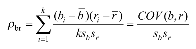
ρ_{br} = {\sum^{​}}_{i = 1}^{k} \frac{(b_{i} - \bar{b}) (r_{i} - \bar{r})}{k s_{b} s_{r}} = \frac{C O V (b, r)}{s_{b} s_{r}}

where $C O V (b, r)$ is the covariance between b and r, $\bar{b}$ and $\bar{r}$ the average responses and reinforcers per window, and s_b and s_r the standard deviations of b and r, respectively.

Following Baum (1973), Dickinson (1985, 1994; Dickinson, Balleine, Watt, Gonzalez, & Boakes, 1995) outlined a correlational-based theory of instrumental goal-directed responding, arguing that goal-directed actions might be assumed to be driven by a mechanism whereby subjects’ experience of the A–O correlation results in the formation of a causal link between the representations of these two events. Although several predictions can be anticipated from this view, the one that is most important for our purposes is the one that anticipates that schedules that bring about positive A–O correlations should support higher levels of responding than those that do not hold this property (Dickinson, 1985, 1994; Dickinson et al., 1995; Kosaki & Dickinson, 2010). Because on ratio schedules response rates are linearly correlated with reinforcement rates, these can be regarded as the cardinal example of such a schedule. Training under RR schedules should thus result in the formation of a causal A–O connection. By contrast, because on interval schedules the relationship between response rate and reinforcement rate is constrained by the programmed interval parameter, these schedules produce low A–O correlations. This, in turn, should result in a weak casual A–O connection. As a result, when presented with a choice test between the RR and the RPI schedules for the same probability of reinforcement, subjects should decide to distribute their responding in favour of the RR schedule because in this scenario a higher correlation implies higher causal control. The approach is also consistent with the results of the first choice test in that participants should prefer the RR with the higher A–O correlation.

Figure 3 shows a simulation of a correlational approach. The left panel shows the correlation coefficient obtained for RR10 and RR30 schedules; the right panel shows the simulation of a master RPI-30 s group and a RR with matched probabilities of reinforcement. The simulations were run assuming an experimental session comprising 360 10-s windows, using a response rate similar to that obtained in the last trial of training of this study (50 responses/min) and a number of simulations equal to the number of data points for each schedule (i.e., 36 subjects per schedule). Although several rules for calculating the correlations are possible—such as considering only a local response rate—for simplicity we calculated the correlations across the whole experimental session simulated. Responding was generated by simulating, for each second, a Bernoulli trial with a constant probability of success equal to .83—so that 50 responses on average were generated in a minute. This implementation ensures that the number of responses varies across windows, and therefore the correlation coefficient can be calculated.

Figure 3.

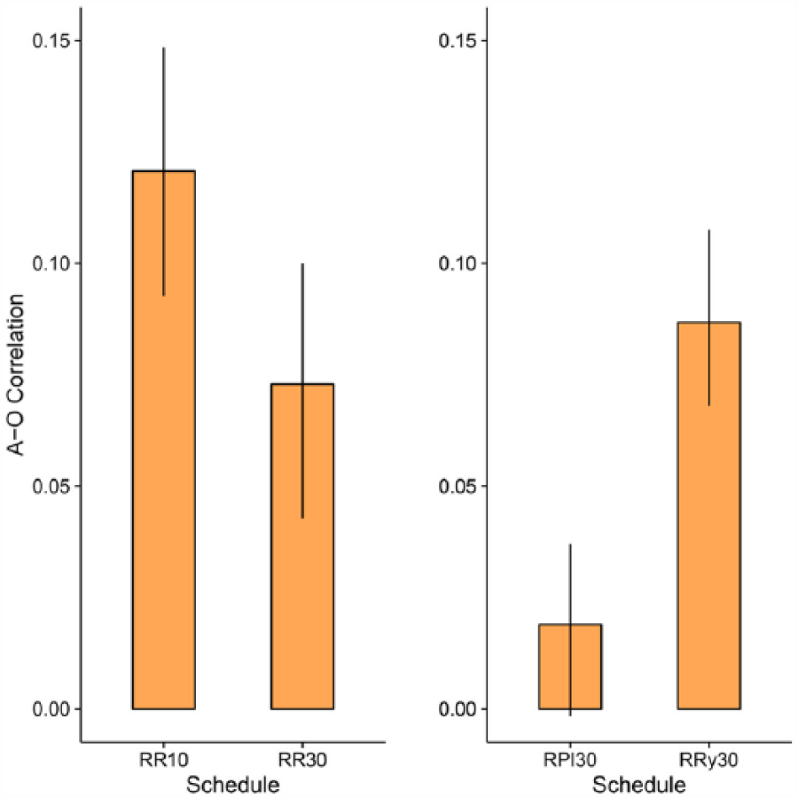
Simulations of a correlational theory of instrumental responding for the present data. RPI = regulated probability interval; RR = random ratio; A–O = action–outcome. Error bars represent 95% confidence intervals.

As can be seen in the figure, a correlational approach offers qualitative predictions in line with the present data: If instrumental responding is a monotonic transformation of the A–O correlation, then subjects should respond more to the RR10 than to the RR30, and more to the RRy30 than to the RPI30.

The correlational approach to goal-directed responding may also shed light into the topic of judgments of causality in humans, where it has been demonstrated that response rates (Shanks, 1993; Shanks & Dickinson, 1991) and also causal judgments of the A–O relationship tend to correlate with the ΔP metric (Chatlosh, Neunaber, & Wasserman, 1985; Dickinson, Shanks, & Evenden, 1984; Shanks, 1991, 1995). In variance with this view, studies on reinforcement schedules have reported both higher response rates and causal ratings for RR than for RI schedules despite having controlled for the probabilities of reinforcement or reinforcement rates (Bradshaw & Reed, 2012; Reed, 2001a, 2001c). The idea of causal control, however, can account for these results by arguing that ratings for ratio schedules are higher due to the higher A–O correlation they support. Likewise, given the low A–O correlation of the RPI schedule, participants should report lower causal ratings on the RPI than on the RR schedule for the same probability of reinforcement. A study by Tanaka, Balleine, and O’Doherty (2008) provided further data in support to this idea. In their study, Tanaka et al. calculated the contingency levels experienced by participants during the task by using a procedure similar to that offered by Baum (1973). This procedure allowed them to show not only that causal ratings were correlated with these different levels, but also that the blood-oxygen-level-dependent (BOLD) signal in the medial prefrontal cortex followed the same pattern, suggesting that such brain structure might be involved in the online computation of an A–O correlation as proposed by Baum (1973).

The role of the A–O correlation as a determinant of instrumental performance has also found support in some studies with human participants using random-interval-plus-linear-feedback (RI+) schedules. RI+ schedules, like standard-interval schedules, differentially reinforce long IRTs, while at the same time instantiating a ratio-like positive A–O correlation, and therefore complement RPI schedules in the analysis of the ratio–interval difference. Whereas a correlational theory of goal-directed behaviour argues that RR schedules maintain a higher response rate than matched RPI schedules, it also anticipates equivalent responding on RR and RI+ schedules. Such equivalence has been reported for the RR–RI+ contrast (McDowell & Wixted, 1986; Reed, 2007a), at least at high response rates (McDowell & Wixted, 1986; Reed, 2007b, 2015).

Whatever the merits of our new experimental design, the present study suggests that the probability of reinforcement might not be the only variable involved in the acquisition of instrumental responding. Although associative theories could provide a reasonable explanation in terms of the representation of the events involved in an instrumental learning scenario, they do not provide an account of the mechanisms involved in the acquisition of instrumental performance in free-operant procedures. In fact, it seems plausible that schedules’ differences are partly brought about by different A–O correlations—or any other extended measure of this relationship—and that this variable is responsible in setting up a causal A–O representation. Our results thus challenge the notion advocated by Mackintosh (1974, 1983) of similar associative processes underlying classical and instrumental conditioning.

Supplemental Material

PQJE_A_1265996_SM0089 – Supplemental material for Human instrumental performance in ratio and interval contingencies: A challenge for associative theory

Supplemental material, PQJE_A_1265996_SM0089 for Human instrumental performance in ratio and interval contingencies: A challenge for associative theory by Mark Haselgrove, IPL McLaren, Omar D Pérez, Michael RF Aitken, Peter Zhukovsky, Fabián A Soto, Gonzalo P Urcelay and Anthony Dickinson in The Quarterly Journal of Experimental Psychology

Footnotes

Acknowledgements

We thank Tor Tarantola for helpful comments on a previous version of this manuscript.

Disclosure statement

No potential conflict of interest was reported by the authors.

Supplementary Material

Supplemental material is available at: .

References

Baum

W. M.

(1973). The correlation-based Law of effect. Journal of the Experimental Analysis of Behavior, 20(1), 137–153.

Bradshaw

C. M.

Freegard

Reed

(2015). Human performance on random ratio and random interval schedules, performance awareness and verbal instructions. Learning & Behavior. doi:10.3758/s13420-015-0178-x

Bradshaw

C. M.

Reed

(2012). Relationship between contingency awareness and human performance on random ratio and random interval schedules. Learning and Motivation, 43(1–2), 55–65. doi: 10.1016/j.lmot.2011.11.002

Cardinal

R. N.

Aitken

M. R. F.

(2010). Whisker: A client-server high-performance multimedia research control system. Behavior Research Methods, 42(4), 1059–1071. doi: 10.3758/BRM.42.4.1059

Catania

A. C.

Matthews

T. J.

Silverman

P. J.

Yohalem

(1977). Yoked variable-ratio and variable-interval responding in pigeons. Journal of the Experimental Analysis of Behavior, 28(2), 155–161.

Chatlosh

D. L. L.

Neunaber

D. J. J.

Wasserman

E. A. E.

(1985). Response-outcome contingency: Behavioral and judgmental effects of appetitive and aversive outcomes with college students. Learning and Motivation, 16(1), 1–34. doi: 10.1016/0023-9690(85)90002-5

Daw

Doya

(2006). The computational neurobiology of learning and reward. Current Opinion in Neurobiology, 16(2), 199–204. doi: 10.1016/j.conb.2006.03.006

Daw

Niv

Dayan

(2005). Uncertainty-based competition between prefrontal and dorsolateral striatal systems for behavioral control. Nature Neuroscience, 8(12), 1704–1711. doi: 10.1038/nn1560

Dawson

G. R.

Dickinson

(1990). Performance on ratio and interval schedules with matched reinforcement rates. The Quarterly Journal of Experimental Psychology, 42(3), 225–239. doi:10.1080/14640749008401882

10.

Dezfouli

Balleine

(2012). Habits, action sequences and reinforcement learning. European Journal of Neuroscience, 35(7), 1036–1051. doi: 10.1111/j.1460-9568.2012.08050.x

11.

Dezfouli

Balleine

(2013). Actions, action sequences and habits: Evidence that goal-directed and habitual action control are hierarchically organized. PLoS Computational Biology, 9(12), e1003364. doi: 10.1371/journal.pcbi.1003364

12.

Dickinson

(1985). Actions and habits: The development of behavioural autonomy. Philosophical Transactions of the Royal Society B: Biological Sciences, 308(1135), 67–78.

13.

Dickinson

(1994). Instrumental conditioning. In Mackintosh

(Ed.), Animal cognition and learning (pp. 45–78). London: Academic Press.

14.

Dickinson

Balleine

Watt

Gonzalez

Boakes

R. A.

(1995). Motivational control after extended instrumental training. Animal Learning & Behavior, 23(2), 197–206. doi: 10.3758/BF03199935

15.

Dickinson

Peters

Shechter

(1984). Overshadowing of responding on ratio and interval schedules by an independent predictor of reinforcement. Behavioural Processes, 9, 421–429.

16.

Dickinson

Shanks

D. R.

Evenden

(1984). Judgement of act-outcome contingency: The role of selective attribution. The Quarterly Journal of Experimental Psychology, 36A(1), 37–41. doi:10.1080/14640748408401502

17.

Dickinson

Watt

Griffiths

W. J. H.

(1992). Free-operant acquisition with delayed reinforcement. The Quarterly Journal of Experimental Psychology Section B: Comparative and Physiological Psychology, 45(3), 241–258. doi:10.1080/14640749208401019

18.

Hammerl

(1993). Blocking observed in human instrumental conditioning. Learning and Motivation, 24, 73–87.

19.

Kass

R. E.

(1993). Bayes factors in practice. The Statistician, 42(5), 551–560. Retrieved from https://classes.warnercnr.colostate.edu/bayes-workshop/files/2013/04/Kass_Statistician_1993_BayesFactors.pdf

20.

Killeen

P. R.

(1994). Mathematical principles of reinforcement. Behavioral and Brain Sciences, 17(1), 105. doi: 10.1017/S0140525X00033628

21.

Killeen

P. R.

Sitomer

M. T.

(2003). Mpr. Behavioural Processes, 62(1–3), 49–64. doi: 10.1016/S0376-6357(03)00017-2

22.

Kosaki

Dickinson

(2010). Choice and contingency in the development of behavioral autonomy during instrumental conditioning. Journal of Experimental Psychology: Animal Behavior Processes, 36(3), 334–342. doi:10.1037/a0016887

23.

Kuch

Platt

J. R.

(1976). Reinforcement rate and interresponse time differentiation. Journal of the Experimental Analysis of Behavior, 26(3), 471–486.

24.

Mackintosh

N. J.

(1974). The psychology of animal learning. San Diego, CA: Academic Press.

25.

Mackintosh

N. J.

(1975). A theory of attention: Variations in the associability of stimuli with reinforcement. Psychological Review, 82(4), 276–298. doi: 10.1037/h0076778

26.

Mackintosh

N. J.

(1983). Conditioning and associative learning. book, Oxford: Clarendon Press.

27.

Mackintosh

N. J.

Dickinson

(1979). Instrumental (type II) conditioning. In Mechanisms of learning and motivation (pp. 143–167). Hillsdale, NJ: Erlbaum.

28.

McDowell

J. J.

Wixted

J. T.

(1986). Variable-ratio schedules as variable-interval schedules with linear feedback loops. Journal of the Experimental Analysis of Behavior, 46(3), 315–329. doi: 10.1901/jeab.1986.46-315

29.

Niv

(2007). Cost, benefit, tonic, phasic: What do response rates tell us about dopamine and motivation? Annals of the New York Academy of Sciences, 1104, 357–376. doi: 10.1196/annals.1390.018

30.

Niv

Daw

Dayan

(2005). How fast to work: Response vigor, motivation and tonic dopamine. Advances in Neural Information Processing Systems, 18(NIPS 2005), 1019–1026.

31.

Niv

Daw

Joel

Dayan

(2007). Tonic dopamine: Opportunity costs and the control of response vigor. Psychopharmacology, 191(3), 507–520. doi: 10.1007/s00213-006-0502-4

32.

Pearce

J. M.

Hall

(1980). A model for pavlovian learning: Variations in the effectiveness of conditioned but not of unconditioned stimuli. Psychological Review, 87(6), 532–552. doi: 10.1037/0033-295X.87.6.532

33.

Peele

D. B.

Casey

Silberberg

(1984). Primacy of interresponse-time reinforcement in accounting for rate differences under variable-ratio and variable-interval schedules. Journal of Experimental Psychology: Animal Behavior Processes, 10(2), 149–167.

34.

Reed

(2001a). Human response rates and causality judgments on schedules of reinforcement. Learning and Motivation, 32(3), 332–348. doi: 10.1006/lmot.2001.1085

35.

Reed

(2001b). Human schedule performance with hypothetical monetary reinforcement. European Journal of Behavior Analysis, 2(2), 225–234.

36.

Reed

(2001c). Schedules of reinforcement as determinants of human causality judgments and response rates. Journal of Experimental Psychology: Animal Behavior Processes, 27(3), 187–195. doi:10.1037//0097-7403.27.3.187

37.

Reed

(2007a). Human sensitivity to reinforcement feedback functions. Psychonomic Bulletin & Review, 14(4), 653–657. doi: 10.3758/BF03196816

38.

Reed

(2007b). Response rate and sensitivity to the molar feedback function relating response and reinforcement rate on VI+ schedules of reinforcement. Journal of Experimental Psychology: Animal Behavior Processes, 33(4), 428–439. doi:10.1037/0097-7403.33.4.428

39.

Reed

(2015). Rats show molar sensitivity to different aspects of random-interval-with-linear-feedback-functions and random-ratio schedules. Journal of Experimental Psychology: Animal Learning and Cognition, 41(4), 432.

40.

Rescorla

R. A.

Wagner

(1972). A theory of Pavlovian conditioning: Variations in the effectiveness of reinforcement and nonreinforcement. Classical Conditioning II: Current Research and Theory, 2, 64–99.

41.

Rouder

J. N.

Speckman

P. L.

Sun

Morey

R. D.

Iverson

(2009). Bayesian t tests for accepting and rejecting the null hypothesis. Psychonomic Bulletin & Review, 16(2), 225–237.

42.

Shanks

D. R.

(1991). On similarities between causal judgments in experienced and described situations. Psychological Science, 2(5), 341–349. doi: 10.1111/j.1467-9280.1991.tb00163.x

43.

Shanks

D. R.

(1993). Human instrumental learning: A critical review of data and theory. British Journal of Psychology, 84(3), 319–354.

44.

Shanks

D. R.

(1995). Is human learning rational? The Quarterly Journal of Experimental Psychology Section A, 48(2), 257–279. doi: 10.1080/14640749508401390

45.

Shanks

D. R.

Dickinson

(1991). Instrumental judgment and performance under variations in action-outcome contingency and contiguity. Memory & Cognition, 19(4), 353–360. doi: 10.3758/BF03197139

46.

St. Claire-smith

(1979). The overshadowing of instrumental conditioning by a stimulus that predicts reinforcement better than the response. Animal Learning & Behavior, 7(2), 224–228.

47.

Tanaka

S. C.

Balleine

O’Doherty

J. P.

(2008). Calculating consequences: Brain systems that encode the causal effects of actions. The Journal of Neuroscience : The Official Journal of the Society for Neuroscience, 28(26), 6750–6755. doi: 10.1523/JNEUROSCI.1808-08.2008

48.

Tanno

(2008). Rational human behavior in schedules of reinforcement. In CARLS series of advanced study of logic and sensibility (pp. 151–158). Centre for Advanced Research on Logic and Sensibility. The Global Centers of Excellence Program, Keio University.

49.

Tanno

Sakagami

(2008). On The primacy of molecular processes in determining response rates under variable-ratio and variable-interval schedules. Journal of the Experimental Analysis of Behavior, 89(1), 5–14. doi: 10.1901/jeab.2008.89-5

50.

Tanno

Silberberg

(2012). The copyist model of response emission. Psychonomic Bulletin & Review, 19(5), 759–778. doi: 10.3758/s13423-012-0267-1

51.

Thomas

(1981). Contiguity, reinforcement rate and the law of effect. The Quarterly Journal of Experimental Psychology, 33(1), 33–43.

52.

Vogel

E. H.

Castro

M. E.

Saavedra

M. a.

(2004). Quantitative models of Pavlovian conditioning. Brain Research Bulletin, 63(3), 173–202. doi: 10.1016/j.brainresbull.2004.01.005

53.

Wagner

Logan

Haberlandt

(1968). Stimulus selection in animal discrimination learning. Journal of Experimental Psychology, 76(2), 171–180. doi: 10.1037/h0025414

54.

Wagner

A. R.

(1969). Stimulus validity and stimulus selection in associative learning. In Mackintosh

N. J.

Honig

W. K.

(Eds.), Fundamental issues in associative learning. Halifax, Canada: Dalhousie University Press.

55.

Wearden

J. H.

Clark

R. B.

(1988). Interresponse-time reinforcement and behavior under aperiodic reinforcement schedules: A case study using computer modeling. Journal of Experimental Psychology: Animal Behavior Processes, 14(2), 200–211. doi:10.1037//0097-7403.14.2.200

56.

Zuriff

G. E.

(1970). A comparison of variable-ratio and variable-interval schedules of reinforcement. Journal of the Experimental Analysis of Behavior, 13(3), 369–374.

Supplementary Material

Please find the following supplemental material available below.

For Open Access articles published under a Creative Commons License, all supplemental material carries the same license as the article it is associated with.

For non-Open Access articles published, all supplemental material carries a non-exclusive license, and permission requests for re-use of supplemental material or any part of supplemental material shall be sent directly to the copyright owner as specified in the copyright notice associated with the article.

0.00 MB

0.04 MB