Compliant-poroelastic lubrication in cartilage-on-cartilage line contacts

Abstract

The mechanisms of friction in natural joints are still relatively unknown and attempts at modelling cartilage-cartilage interfaces are rare despite the huge promise they offer in understanding bio-friction. This article derives a model combining finite strain, porous and thin-film flow theories to describe the lubrication of cartilage-on-cartilage line contacts. The material is modelled as compliant and poroelastic in which the micro-scale fibrous structure is interstitially filled with synovial fluid. This fluid flows over the interface between the bodies and is coupled to pressure generated by relative motion in the thin-film region formed under load. A Stribeck analysis demonstrated that this type of contact is determinable to conventional elastic lubrication but that the friction performance is improved by this interfacial flow. Moreover, the inclusion of periodic flow conditions when contact is onset is a specific novelty which elucidates new observations in the lubrication mechanisms pertaining to natural joints.

Keywords

Poroelasticity lubrication compliance cartilage friction

1 Introduction

The interface of mammalian articular joints is comprised of opposing cartilage layers which allow for sliding under shock and cyclic loads with very low friction [1 –3]. Degradation of the cartilage surfaces due to degenerative diseases, such as osteoarthritis, affects around 3.3% of the works population. Joint pain, stiffness, swelling and decreased range of motion are common symptoms associated with the disease. Whilst non-invasive treatment methods exist to combat pain and discomfort, joint replacement is common tool to symptoms. The cartilage can be conceptualised as a compliant-poroelastic material containing a fluid phase and a solid matrix which frustrates the free movement of fluid creating transient pressure responses to deformation [4 –7]. The fluid acts as the primary load bearing medium when the surfaces are in motion, but when the movement is slow or stationary loads are transferred to the solid matrix as the fluid migrates out of the high pressure regions [8,9]. Maintaining a significantly pressurised fluid is dependent on whether the forces induced by advection of the material as it undergoes deformation are significantly larger than those due to diffusion of the fluid within the material due to porous flow. This results in a high Peclet number for the contact with this behaviour, referred to in the literature as migrating contact, contributing to the remarkable load carrying capacity [10 –12] and the ability to maintain a well lubricated interface for sustained use [13,14]. At the cartilage surface fluid is free to traverse the boundary in response to a load differential across that boundary. This allows for the tribological rehydration process whereby fluid in the converging wedge is drawn into the poroelastic medium from the surrounding bath [15,16]. Whilst the hydration of the cartilage tissues has been noted as an important contributor to lubrication, it has been hypothesised recently that it is equally important to the preservation of joint space and ultimately joint health [15].

Biot [17] created an early description of fluid flow in a poroelastic solid and subsequent investigators have since built on this to model articular cartilage [5,18 –20]. Estimates for the material properties have been derived from experimental compression testing [9,21,22] and from magnetic resonance imaging [23]. High fidelity models focusing on the bio mechanics of a single joint have utilised commercial finite element packages to understand how the cartilage is externally loaded by the relative motion of bone [24 –27].

While it is clear that the lubrication processes at the boundary are complex, it has been shown that the resulting friction coefficients from a cartilage-on-glass case form a Stribeck curve similar to those in non-porous materials [28]. Soft fluid-filled porous materials of this nature have been modelled by coupling the continuum mechanics that describe a compliant-poroelastic material with thin-film theory to describe the lubricating boundary [29,30]. Recently, this was expanded to include a Stribeck type analysis of a compliant-poroelastic (or porohyperelastic) material rotating against an impermeable surface to show that the lubrication modes (boundary, mixed and hydrodynamic) can be predicted at given operating conditions [31]. The present work performs a similar Stribeck type analysis on two contacting compliant-poroelastic layers. Replacing the impermeable wall with a compliant-poroelastic surface allows fluid to flow across the contacting boundaries and for mutual deformation in response to contact, friction and lubricating loads. This more closely represents the tribological reality in a natural joint and is achieved using a periodic flow boundary condition at the interface in the fluid phase. This condition is the novel contribution of this work which facilitates a step-change in the state-of-the-art modelling capacity for cartilage interactions in natural joints.

2 Materials and methods

This section provides a definition of the problem in terms of cartilage-on-cartilage contacting in the natural joint, outlines the theory of compliant-poroelastic lubrication, the numerical procedure implemented to solve the problem and defines the case study investigated in the remainder of the article.

2.1 Problem definition

In this article, the compliant-poroelastic lubrication of cartilage-on-cartilage is considered where two bodies rotate under load in a line contact geometry. For this purpose, a 2D cross-section through the geometry is modelled and the governing equations derived. The geometry is defined in the - plane in which the size of the body considered in the out-of-plane direction is orders of magnitude larger than in either of the or directions. The contacting interfaces are assumed to be perfectly smooth, the material properties are isotropic and do not vary within the compliant-poroelastic material.

Figure 1 shows the problem geometry where two bodies ABCD and EFGH represent converging-diverging wedges of cartilage, both with outer and inner radii of and , respectively, rotating at axial speeds of and about their corresponding centres . The boundaries AD, BC, EH and FG of the cartilage bodies extend far enough from the centre such that they do not affect the results generated in the contact region. A sector angle of specifies the pre-deformation geometry of the bodies which both have a line of symmetry at x = 0. The backing of the cartilage bodies CD and GH are assumed to be in contact with rigid bone within the natural joint and as such they are impermeable and do not deform.

Figure 1

Sketch of the compliant-poroelastic lubrication of two curved articular cartilage bodies rotating under load. In the case shown the penetration depth , deformation of the contacting interface is included, and a full film of thickness is formed.

The boundaries AB and EF represent the lubricated interface of cartilage-on-cartilage, surface texture and/or roughness of these surface is not included in the model. This forms a line contact problem in which a lubricated film of thickness is created between the surfaces, additional constraints apply due to flow between the lubricating region and the cartilage bodies. The boundaries AB and EF can also be in solid contact depending on the magnitude of the load carried, when the bodies contact there is a transition from fluid film lubrication to periodic fluid flow across the porous interface. The total load carried is , which is the load due to fluid pressure and solid normal stress acting on AB and EF, respectively. The subscripts 1 and 2 are used throughout this article to distinguish between variables related to the bodies ABCD and EFGH, respectively, giving the total load on ABCD as and EFGH as . To generate this, the bodies are deformed by an increment of about the line y = 0 such that they contact with a penetration depth of . For negative penetration depths a full fluid film is formed, as decreases to zero and then becomes positive surface deformation is generated and a full fluid film is maintained, subsequently as becomes more positive solid contact of the interface onset.

2.2 Compliant-poroelastic lubrication

In this model cartilage is considered biphasic in which the solid fibrous material deforms under load and is interstitially pressurised by a fluid filling the pores. The poroelastic description of cartilage is well-established as an accurate means of capturing the behaviour of the material under load [5,6]. Compliant-poroelasticity or porohyperelasticity is of specific interest because cartilage experiences large deformations during operation in the natural joint, therefore, compliance must be considered in any model describing this complex fluid–structure interaction phenomenon [18]. In the following subsections, compliant-poroelastic lubrication is described in which the combined theories of finite strain, porous flow and thin-film flow form a mechanism describing the functionality of cartilage in natural joints. A steady-state assumption is applied to the model derived by de Boer et al. [31] for cartilage against a rigid impermeable surface. This is then expanded for the contact of two compliant-poroelastic bodies, elucidating the lubrication mechanisms for cartilage-on-cartilage contacts under representative constant load and axial speed conditions.

2.2.1 Solid mechanics

Finite strain theory is invoked to derive the equation of state for the compliant solid phase, the generation of stress is subsequently coupled to fluid pressurisation to form the compliant-poroelastic response. This results in Equation (1) which describes the conservation of energy in the solid phase coupled to the body force generated by fluid pressurisation. The equation of state for the solid phase is derived based on the definition of the Biot-Willis parameter and the strain energy density . The Biot-Willis coefficient is a fundamental constant used in the definition of poroelasticity in order to account for the compressibility of the solid and fluid phases, respectively, [17]. The strain energy density is used to define the hyperelastic response of the solid deformation in which the stress–strain relationship for the material is obtained by the derivative of strain energy density with respect to strain [32]. This expands on the concept of linear poroelasticity established for cartilage like materials by Mow et al. [5,6] toward finite deformations and compliant materials as implemented by Simon [18] and more recently by de Boer et al. [31] with respect to rotating interfaces and lubrication.

In Equation (1), is the solid deformation, is the fluid pressure, is the deformation gradient tensor and is the 2nd Piola-Kirchhoff stress tensor. Where is the identity tensor, is the strain tensor, and is the right Cauchy-Green deformation tensor. Due to the 2D nature of the problem, plane strain assumptions apply for the solid phase. When the body force due to fluid pressure is neglected or , only the solid phase is considered and subsequently Equation (1) becomes exactly the equation for the conservation of energy in a compliant solid material.

(1)

The strain energy density for the solid phase considers two terms as described by Equation (2), where is the isochoric strain energy density and is the volumetric strain energy density. To generate a representative strain energy density for the compliant solid phase a metric to a simplified hyperelastic model is used. This can be replaced by any suitable definition so long as the constants used to describe the response can be obtained by physical testing. Here only the drained shear modulus and drained bulk modulus are needed, both of which can be obtained for the drained solid phase. Drained means that these material properties are measured when the fluid has been entirely exuded from the porous material and only the solid phase is considered.

By implementing the compressible Neo-Hookean hyperelastic model the isochoric and volumetric strain energy density functions for the solid phase are given, respectively, by Equations (3) and %(4). In which, is the volume ratio, is the 1st invariant of the isochoric part of the right Cauchy-Green deformation tensor and is the 1st invariant of the right Cauchy-Green deformation tensor. The Cauchy stress tensor is also defined by and from which the von Mises’ stress is obtained as the tensor magnitude . (2) (3) (4)

The volume ratio is used to couple changes in the solid volume to the generation of pressure as described in Section 2.2.2. The Biot-Willis coefficient varies between 0 and 1, with a value of 1 meaning that any change in the volume of the solid produces the same change in volume of the fluid. When there is no contribution to volumetric changes in the fluid as the solid volume changes. Where there is both volumetric changes to both the solid (through volumetric strain) and fluid (through volumetric flow) phases.
2.2.2 Fluid mechanics

Conservation of mass in the fluid phase leads to the derivation of the governing equation for the pressure, this is coupled to changes in volume of the solid to form the compliant-poroelastic response. Equation (5) describes the porous fluid flow in the fluid phase and a term describing the change in volume of the solid due to motion of the bodies through space which results from the steady-state form of the material derivative. Where in Equation (5), is the fluid density, is the fluid velocity and is the velocity of the bodies. The fluid velocity is generated proportionally with the pressure gradient which results in the definition of the material intrinsic permeability . This, in combination with the dynamic viscosity , produces a viscous porous flow as given by Darcy's law, this is well-established mechanism for describing the transport of synovial fluid in cartilage [33]. The fluid is also linearly compressible where , in which is the density at zero pressure and is the fluid compressibility. The velocity of the bodies is comprised of two terms, the translational velocity and the rotational velocity 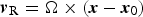. 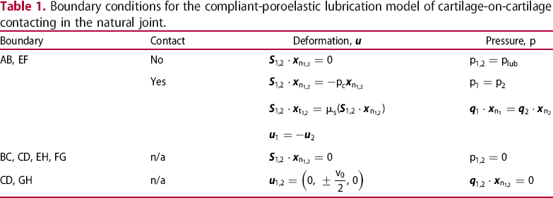Here the translation of the body is zero and the rotation is defined by as the axial velocity, is the position vector and 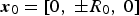are the locations of the centres of rotation in the material frame of reference. The rotational velocity of the two bodies are different as they rotate about different centres with different axial speeds, hence subscripts 1 and 2 are used to distinguish between ABCD and EFGH, respectively.

(5)
2.2.3 Boundary conditions

Boundary conditions are specified for the solid and fluid governing equations, these must describe the representative behaviour of the cartilage material as it rotates under load in lubricated conditions. Table 1 gives these conditions for the solid deformation

and fluid pressure

at each boundary,

and

are the surface normal and tangential unit vectors, respectively, the normal direction is orientated in the outward facing direction of the bodies and the tangential direction is orientated in the positive direction of sliding.

Table 1
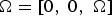
Boundary conditions for the compliant-poroelastic lubrication model of cartilage-on-cartilage contacting in the natural joint.

Boundary	Contact	Deformation,	Pressure,
AB, EF	No
AB, EF	Yes
BC, CD, EH, FG	n/a
CD, GH	n/a

Note that when contact occurs boundaries AB and EF are both within and outside the contacting region. When there is no contact the pressure acting on AB and EF is that due to the thin-film lubrication alone and is described in detail in Section 2.2.4, corresponding to this a free deformation (or zero traction) condition is applied to the solid. If contact does occur then the condition for the fluid phase becomes periodic in the contact region as fluid moves across the interface, outside the contact region the pressure remains that of the lubricating pressure. The solid condition in the contact region is dictated by contact mechanics as described in more detail in Section 2.2.5, outside the contact region it remains free to deform. Boundaries CD and GH are considered impermeable and as such zero fluid flow conditions are applied, for the solid phase these boundaries deform in the vertical direction by , respectively, to generate the total load carried (see Section 2.2.6), they are constrained to zero in the remaining directions. The boundaries BC, CD, EH and FG are assumed far enough from the centre of the contact such that a zero or ambient pressure condition is applicable, for the solid phase they can freely to deform.

2.2.4 Thin-film flow

Within the region between boundaries AB and EF a thin-film fluid flow is assumed to form, the Reynolds approximation is invoked to reduce the dimension of the thin-film governing equation by neglecting derivatives across the film thickness. This facilitates the formation of a governing equation for the lubricating pressure arising from the thin-film acting in the horizontal direction of sliding motion. This is a valid approach so long as the radii of the contacting bodies are orders of magnitude larger than the vertical distance between the two surfaces. The vertical distance between AB and EF is the film thickness as given by . Fluid is also transported in vertical direction through the porous interfaces, the lubricating flow is subsequently coupled to the fluid flow into and out of the compliant-poroelastic bodies by an additional source term. This results in Equation (6) and Equation (7) for the transport of fluid in the thin-film region, where is the volumetric flux (per unit depth), is the horizontal component of the tangential surface direction , is the fluid flow into and out of the porous interfaces and is the interfacial sliding speed. Zero pressure boundary conditions are applied at the locations A, B, E and F to correspond to those connecting boundaries outlined in Table 1. Hydrodynamic cavitation of the fluid phase is not considered as the pressures experienced remain significantly above the saturated vapour pressure [34]. However, it is possible that a free surface, and therefore pressure due to interfacial surface tension, is present at the diverging region. This presents challenges not only in the consideration of the free surface in the fluid film region but also potentially where fluid is drawn back into the porous material and the interaction of the free surface with the material pores [35]. It is therefore assumed that the gap between the porous surfaces is fully flooded.

(6) (7) The horizontal tangential direction is different for the two bodies due to the alignment of the geometry about the line of symmetry x = 0. Therefore, for AB a positive . is the same as the positive direction of sliding and that for EF a positive is the same as the negative direction of sliding, with the positive direction of sliding corresponding to the positive horizontal axis y = 0. As such for EF a scaling of −1 is applied to the derivative terms of Equations (6) and %(7) to formulate the correct lubricating pressure acting on both boundaries. The sliding speed is given by , in which the sliding speeds of each body are , respectively, due to the difference in the direction of positive rotation at the interface and the positive direction of sliding.

The fluid flow into and out of the porous interfaces is also different on and AB and EF due to the opposite alignment of the normal outward facing direction of the two bodies. As such on AB, and on EF, . Each of these flows correspond to the surface flux of porous fluid flow within each of the bodies, , obtained from the fluid phase. This creates a coupling between the pressure and pressure gradient acting on AB and EF and the additional challenge of solving the thin-film flow equations with the compliant-poroelastic equations. The result of this is that the lubricating pressure produced is identical in distribution and magnitude on AB and EF, whereas the distributions of the lubricating flux and interfacial flow acting on AB and EF are identical in distribution but opposite in sign. In the case where contact occurs and the film thickness is zero , there can be no lubricating flow as is obtained from Equation (7). Within this region the pressure remains identical on either side of the interface, , and the normal fluid flow across the interface becomes equal, . This subsequently leads to a periodic flow condition for the fluid flowing through the bodies at the contacting interface as described in Table 1.
2.2.5 Contact mechanics

A contact pressure is generated between the two bodies while in contact. This is calculated according to the required penetration of the bodies, which is in turn dictated by the magnitude of deformation of the contacting interfaces under load and the penetration depth . The contact pressure applies a normal stress to the solid phase ensuring that the penetration of the bodies is zero, corresponding to this is a tangential stress due to friction generated between the solid-on-solid contact. For this purpose, a dry cartilage-on-cartilage coefficient of friction is specified which describes the proportion of tangential solid load to normal solid load at the interface between the two solid bodies when all fluid has been exuded (drained conditions). The distribution of contact pressure generated on either side of the contact is identical, however, there will be differences in the resulting solid stress distributions at the interface if the material properties of the touching bodies vary.

When the two bodies are in contact the film thickness is zero and this forms a contact region of length along the line y = 0. As such the minimum film thickness is always equal to zero when the two surfaces are in contact, however, this does not always relate to a positive penetration depth as surface deformation occurs. Therefore, remains positive until the total load cannot be maintained and contact is onset. This means that the contact length becomes positive when is zero, note that this does not correspond with the expected penetration length . The resulting condition for the solid deformation is anti-periodic at the interface, where the two bodies form the contacting region along y = 0.

The penetration length is given by , where is the Heaviside function. This gives the length of the contacting region when deformation of the interfaces is not considered, see Figure 2(a). This measurement facilitates an analysis how out of shape the contact length , which includes surface deformation, becomes in comparison to the size of the penetration . The contact length is determined by Equation (8), where and are angles swept out by the contacting region on the left-hand-side and right-hand-side of the vertical axis, respectively. These can be expressed in terms of the arc length of either body within the contact region, and , as given on the left-hand-side and right-hand-side of the vertical axis, respectively. These are by Equations (9) and %(10), where either boundary AB or EF can be considered for conducting the integration. The term is the Delta function of the film thickness and produces a value of unity where the film thickness is zero and contact is onset. For reference the arc length of each boundary are equal to at A or E, at [0, ], and at B or F. The contact length must be calculated using this approach because the region over which the film thickness is zero is not symmetrical about the vertical axis due to deformation of the interface under load, as shown in Figure 2(b).

(8) (9) (10)
Figure 2
Sketch of the two cartilage bodies in contact showing the definitions of: (a) the penetration length where deformation is not included; and (b) the contact length where deformation is included. In both cases the penetration depth is positive .
2.2.6 Load capacity

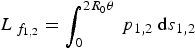
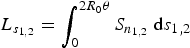
The total load capacity (per unit depth) is given by the loads acting on AB and EF but it is also the sum of fluid load and solid load acting on either surface, and . Subsequently these are related by considering the individual contributions of the fluid pressure and solid stress acting on AB and EF, giving , and . Each of the individual contributions is described in Equations (11) and %(12) and is obtained by integrating the fluid pressure and magnitude of the solid normal stress distributions over each boundary. As such the individual load contributions for both the fluid and solid phases are equal on each body as the same pressure and normal stress is applied to both AB and EF. The total load varies monotonically with the penetration depth and as such the determination of contact or full fluid film behaviour is described by variance of either parameter.

(11) (12)

The Sommerfeld number is defined by and is used in the analysis of load variation of line contact geometries to establish the different lubrication regimes observed. Two further parameters are also introduce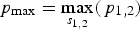d and 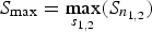which describe the maximum value of the fluid pressure and magnitude of the solid normal stress acting on either AB or EF, respectively.
2.2.7 Friction

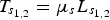
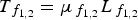
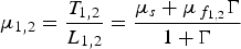
When contact mechanics was considered in Section 2.2.5 a coefficient of friction was specified for the contact between the solid cartilage-on-cartilage interface in drained conditions. This differs to the coefficient of friction of the compliant-poroelastic contact which also includes the influence of shear stresses due the fluid flow. The compliant-poroelastic coefficients of friction are given by Equation (13), the friction is different on AB and EF because the fluid shear stress varies with the film thickness. In Equation (13), 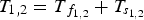are the total tangential loads, are the fluid tangential loads and are the solid tangential loads each acting on AB and EF respectively. Subsequently, are the solid tangential loads, are the fluid tangential loads and are the coefficients of friction due to fluid flow acting on AB and EF respectively. Additionally, the parameter is defined as the ratio of the fluid load to solid load in the contact.

(13)

The fluid tangential loads are given by integration of the fluid shear stress acting along AB and EF. This results in Equation (14) and Equation (15) which, respectively, describe the fluid tangential loads and shear stress of the fluid acting on both surfaces as derived from thin-film flow theory. Due to the alignment of tangential directions being opposite on AB and EF the derivative term of Equation (15) for EF is scaled by −1, which is consistent with the method applied to the fluid flow equations as described in Section 2.2.4. In Equation (15), is the slide-to-roll ratio. It is of note that the second term on the right-hand-side of Equation (15) contains which tends to infinity when the film thickness is zero and contact is onset. However, when the slide-to-roll ratio is zero, , then this term becomes zero in the fluid shear stress calculation and the problem of the infinitely thin film can be neglected. Also, in this case the fluid tangential loads become , leading to and . (14) (15)

A zero slide-to-roll ratio is only examined in this article, however, de Boer et al. [31] used a limiting film thickness approach to resolve the problem in relation to the contact of a compliant-poroelastic material against a rigid impermeable surface. This method sets a minimum film thickness for the term in question and as a result a maximum fluid shear stress is generated within an infinitely thin film. The scale over which the limiting film thickness should be specified is somewhat arbitrary and this has been previously examined by authors who link it to the size of surface asperities in elastic materials. These models are yet to establish a means of incorporating porous flow over the contacting interface between asperities and as such no technique is necessarily applicable to the compliant-poroelastic model presented here.
2.3 Numerical method

The finite element (FE) method, as implemented in the software Comsol Multiphysics v3.5a, was used to solve the problem outlined in Section 2.2. This package provides the necessary tools for coupling the solid, fluid and thin-film flow components of the model.

2.3.1 Discretisation

The two bodies ABCD and EFGHG were each discretised with quadrilateral elements, with elements distributed elements evenly along all the lengths. Grid independent results were observed when the number of elements on AB/CD/EF/GH was 300 and on AD/BC/EH/FG was 30. This produced a mesh with a total of 18,000 elements, in which 9000 elements discretised each of the bodies independently. The same mesh was used for all simulations conducted. The compliant-poroelastic domains were discretised with 2D elements, this subsequently meant that 1D elements discretised the thin-film flow domains AB and EF. For each of the governing equations specified, 2nd order polynomial shape functions were used to generate the elemental equations and formulate the finite element matrix problem. This was subsequently solved using the numerical algorithms provided with the software to provide the distributions of solid stress and fluid pressure throughout the numerical domains.

2.3.2 Solution procedure

To solve the model numerically a single initialisation step was required to generate solutions for a given penetration depth . This step was needed to ensure that the initial solution provided was significantly closer to the final solution than zero distributions of solid stress and fluid pressure. It was found that a zero solution would cause the solver to diverge unless the contact mechanics was solved without the thin-film flow equations previously. This was due to a high sensitivity of the solution to the lubricating pressure provided at AB and EF when contact mechanics was included, where there is also a strong coupling to the fluid flow to and from the porous interface. Therefore, the initialisation step did not include the thin-film flow equations and instead a no flux boundary condition was applied to both AB and EF. Subsequently, this solution was used as the initial solution to the solid stress and fluid pressure when the thin-film flow equations were then also included. In the case where there is no penetration this step was not necessary as contact mechanics were not required. An iterative solver was subsequently used to solve the FE matrix problem and satisfy the requirements of contact mechanics if applicable. This was achieved using a penalty type algorithm to solve for the contact pressure. In which two model constants were needed, the contact stiffness and initial contact pressure. These were specified as and , respectively, in accordance with the guidelines provided in the software for use of the penalty algorithm with compliant materials.

2.4 Case study

The case study investigated considers two cartilage bodies under constant load rotating with constant axial speed. For this the material properties, operating conditions and geometrical parameters are presented in Table 2. The geometry defined considers two 1 mm thick layers of cartilage rotating against each other with sliding conditions at the contacting interface between them. These values were chosen to represent the material properties of cartilage and its operation in natural joints. The value chosen for the solid-on-solid coefficient of friction is

was selected based on that of dry cartilage-on-cartilage friction measurements under similar conditions. The high solid friction in such contacts is related to the complete exudation of water within the contact thus leaving the best current value for ‘dry fiction’ as that of two soft elastic bodies, that is the solid coefficient of friction in drained conditions for a compliant-poroelastic material such as cartilage. A zero slide-to-roll ratio has been specified to avoid the fluid shear stress measurement problems as discussed in Section 2.2.7. This results in a constant value of the sliding speed

which is assumed large enough to generate a shear rate which produces a constant viscosity of the fluid (∼10⁵ – 10⁶ s⁻¹). This is an important consideration as the model is derived based on an isoviscous fluid response in which the viscosity of the shear-thinning synovial fluid can be considered constant in value [36].

Table 2
Material properties, geometrical parameters and operating conditions for the case study investigated.

Name	Symbol	Value
Drained shear modulus		0.5 MPa
Drained bulk modulus		5 MPa
Outer radius		100 mm
Inner radius		99 mm
Sliding speed		0.2 m.s⁻¹
Penetration depth		[−100, 10] μm
Biot-Willis coefficient		0.9
Dynamic viscosity		0.001 Pa.s
Sector angle		π/36 rad
Permeability		1 × 10⁻¹⁵ m²
Coefficient of friction (drained solid-on-solid)		0.45
Fluid density at ambient pressure		1000 kg.m⁻³
Fluid compressibility		0.1 GPa⁻¹
Slide-to-roll ratio		0
Axial speed		1 rad.s⁻¹

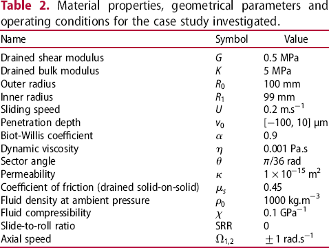
The only parameter allowed to vary in the model is the penetration depth , from which load variation is achieved and subsequently the range of lubrication regimes observed. The range of used is given in Table 2, the parameter was varied with a step size of 1 μm such that a total of 111 simulations were conducted. This means that for the Stribeck analysis presented in Section 3 there is no sliding speed variation only load variation. The simulation time varied exponentially with decreasing when in contact and linearly when contact mechanics was not needed, with the longest simulation taking 3 h 47 min at the minimum and the shortest taking 3 min at the maximum . The total computing time was 76 h 13 min.

3 Results and discussion

Results presented in this section correspond to two different categories. In Section 3.1 a Stribeck analysis of the compliant-poroelastic lubrication model is conducted showing the full range of lubrication regimes experienced under load. Section 3.2 then goes on to explore the results of this analysis in more depth, with each subsection describing the pressure, stress and fluid flow distributions observed in the different lubrication regimes.

3.1 Stribeck analysis

Steady-state simulations were conducted over the specified range of the penetration depth given in Section 2.4, with the corresponding pressure and stress distributions calculated as a result. Post-processing of these simulations allowed the friction, film thickness, contact length, maximum pressure and stress, and the load capacity to be determined, as presented in Figure 3. As part of this Stribeck analysis, it should be noted that the sliding speed is kept constant and that load is the variable parameter, each solution produced represents a different result of the system assuming steady-state conditions.

Figure 3

Stribeck analysis of the compliant-poroelastic lubrication of cartilage-on-cartilage. Showing the variation of the following parameters with the Sommerfeld number : (a) the compliant-poroelastic coefficient of friction , the coefficient of friction due to fluid flow and the ratio of fluid to solid load ; (b) the contact length , penetration length , minimum film thickness and absolute value of the penetration depth ; (c) the maximum pressure on the contacting interface and the maximum normal stress on the contacting interface ; and (d) the fluid load and the solid load .

Figure 3(a) shows the clear definition of the expected lubrication regimes in a conventional line contact, where friction initially reduces with increasing load to a minimum value before sharply increasing as contact is onset. However, the exact values and shape of the response for the compliant-poroelastic materials is significantly different to that of elastic materials in lubricated conditions, which is linked to the flow of fluid through the porous interface. Figure 3(a) indicates that load carried by the fluid is one or two orders of magnitude larger than that of the solid when the friction is low and a full fluid film is generated, and subsequently that in the high friction case that the load capacity of the two phases are of the same order of magnitude with contact onset at the interface. The contribution to friction from the fluid phase is always monotonically decreasing with increasing load, however, due to the biphasic nature of the material the overall friction increases after contact is onset. The minimum coefficient of friction observed was = 0.0053 which occurred the instance before the minimum film thickness reached zero with increasing load and contact occurred.

The contacting interface is deformed significantly according to Figure 3(b), with the difference between the penetration depth and minimum film thickness increasing with load over three orders of magnitude. At the instance that contact would be onset without deformation, , the film thickness is 4 μm, but when contact is onset and the film thickness is zero, 0, then the penetration depth was 13 μm. The contact length sharply increases with load as contact is onset and remains less than the expected penetration length for all loads investigated. The size of the contact region and penetration depths experienced throughout imply that the material deformation is significant (up to 10% of the thickness) and that a compliant model is needed under the loads experienced given the magnitude of the material parameters provided.

The maximum stress and maximum pressure are both monotonically increasing with load as according to Figure 3(c). Before contact occurs, both increase at a steady rate, however, after contact the maximum stress increases at a faster rate (after briefly plateauing during the initial contact) and the maximum pressure increases with a reduced rate. Corresponding to this Figure 3(d) shows that the fluid load is always monotonically increasing at a steady rate despite the onset of contact, whereas the solid load is always monotonically increasing with load but experiences as sharp increase in rate after contact is initiated.

3.2 Lubrication regimes

The following subsections present results relating to each of the lubrication regimes identified in the Stribeck analysis conducted in Section 3.1. Visualisation of the pressure and stress distributions in the two bodies is provided, along with the pressure, stress, film thickness and fluid flow acting on the contacting interface.

3.2.1 Thin-film flow

In this regime a full fluid film is formed between the two bodies, the load carried is low (right-hand-side of Figure 3) and the behaviour can be described as elastohydrodynamic. Figure 4(a) shows that pressure which is generated due to lubricated flow at the contacting interface is built-up in the minimum film thickness region, corresponding to this Figure 4(b) indicates that the solid stress increases in the region either side of the pressure build-up where material is compressed under load and constrained against the cartilage/bone interface. The magnitude of the pressure and stress reached is low (∼0.5 – 1 kPa) and as such the amount of deformation is also low. Figure 5(a) shows that the contacting interface is deformed under the low pressurisation but that this is not distorting the shape of the bodies. Also shown is that while the fluid is pressurised that the solid stress is negligible as contact is not onset. Fluid flows into the material before the constriction as is negative whereas fluid flows out of the material after the constriction where is positive, see Figure 5(b). Corresponding to this the lubricating flux is always positive such that there is always a flow of lubricant in the sliding direction but in the constriction, this is reduced where flow into and then out of the material reach their maximum values.

Figure 4

Distributions within the compliant-poroelastic bodies of: (a) the fluid pressure ; and (b) the solid Mises's stress . In this case the penetration depth is 1 μm.

Figure 5

Distributions along the contacting interface of the compliant-poroelastic bodies showing: (a) the fluid pressure , the solid normal stress and the film thickness ; and (b) the lubricating flux and the fluid flow at the contacting interface . In this case the penetration depth is 1 μm.

3.2.2 Low friction

As the load is increased a full fluid film is maintained between the contacting bodies; significant deformation occurs due to the compliant solid phase and as such a large constriction is formed. Figure 6(a,b) shows that this generates pressure and stresses of the order of ∼10 – 20 kPa which form in the same way as observed in the thin-film flow regime. However, in this case, the solid stress response is more significant with a maximum value forming on the cartilage/bone interface near the centre of the bodies. At the contacting interface there is a significant constriction formed in which the film thickness is always positive but near-zero in value, this where the fluid pressure is built-up much more than in the thin-film flow regime as seen in Figure 7(a). The shape of the pressure distribution is representative of conventional line contact in which after the pressure build-up there is a negative pressure formed to maintain mass conservation in the lubricating film. Figure 7(b) indicates a similar response in terms of the lubricating flux and interfacial flow than for the thin-film flow regimes. The lubricating flux is reduced in value compared to the previous case but is always positive in value, the interfacial flow exhibits the same behaviour where flow is into the material before the constriction and out after the constriction. This interfacial flow is also an order of magnitude larger than in the thin-film flow regime. However, the gradients are much steeper for this regime. The combination of interfacial flow and complaint deformation of the material facilitates the large constriction formed, which in turn results in the generation of small fluid shear stress and the formation of the low coefficients of friction observed in this regime. With the minimum coefficient of friction reached being 0.0053 for the case study investigated.

Figure 6

Distributions within the compliant-poroelastic bodies of: (a) the fluid pressure ; and (b) the solid Mises's stress . In this case the penetration depth is −19 μm.

Figure 7

3.2.3 Boundary contact

A further increase in load from the low friction regime results in boundary contact. In this case, there is no longer a full fluid film formed and instead the constriction reaches zero and contact is onset. Figure 8(a,b) correspondingly shows that the pressure and stress continue to exhibit the same shape of response than in the previous regimes but that they span a larger constriction region. The magnitude of both parameters is also increased and is of the order of ∼50 kPa. The most significant changes are observed at the contacting interface. Figure 9(a) shows that the pressure produces a small spike before the constriction in addition to a positive solid stress (∼10 kPa) being generated where the film thickness is zero. Figure 9(b) shows that the lubricating flux becomes zero where the film is also zero and no flow can occur. In the region before the constriction, the flow is positive and after the constriction a small amount of backflow is experienced before becoming positive again. Corresponding to this the interfacial flow is more complex than for the previous regimes with a different shape of response produced. Flow moves into the body before the constriction and out after the constriction. However, in the latter of these, there is also flow into the body where backflow is predicted in the lubricating line. Within the contacting region, there remains flow across the interface due to the periodic flow conditions formed, this is however significantly lower in magnitude than the flow in the flow across the interface where contact is not onset. In the boundary contact regime both the lubricating flux and interfacial flow are lower than they are in the low friction regime.

Figure 8

Distributions within the compliant-poroelastic bodies of: (a) the fluid pressure ; and (b) the solid Mises's stress . In this case the penetration depth is −48 μm.

Figure 9

3.2.4 High friction

Increasing the load even further results in the high friction regime under contact conditions, in this regime a full fluid film is not formed and the bodies are significantly penetrated into one another. The maximum pressure is shown to be ∼60 kPa and the maximum stress at ∼85 kPa in Figure 10(a,b), respectively, demonstrating that the high friction results in an increase of the solid in the load carrying capacity due to solid-on-solid contact. The shape of the pressure and stress distributions remains similar in shape, spread over a larger contact region. Figure 11(a) indicates that the pressure on the contacting interface maintains the same shape as for the boundary contact regime but only increases to ∼60 kPa whereas the solid stress increases with the size of the contact and reaches ∼40 kPa which is a much larger difference than the pressure compared to the previous regime. The film thickness is zero over a larger contact length and this corresponds to where the solid stress is positive. The lubricating flux and interfacial flow show similar behaviour to that of the boundary contact regime but where the values are significantly larger in magnitude, see Figure 11(b). There is no backflow experienced after the contact region in this case and a zero-flow maintained throughout the contact region. However, there is flow into and out of the material after the contact owing to the complex link with the periodic flow maintained in the contact region. Again, in this regime, the flow across the boundary in the contacting region is less than that experienced across the boundary outside of the contact region. The coefficient of friction in this regime is of the order of ∼0.1 – 0.15.

Figure 10

Distributions within the compliant-poroelastic bodies of: (a) the fluid pressure ; and (b) the solid Mises's stress . In this case the penetration depth is −100 μm.

Figure 11

4 Summary and conclusions

This study set out to address the tribological line contact problem between mating articular cartilage layers with a focus on their mechanical interactions. That is a system where cartilage layers are in a rotational sliding configuration and experience large deformations, which are themselves manifested due to squeeze loading from the relative motion of rigid bone and tangential forces arising from friction induced by sliding at the contacting interface. In addition to the numerical cartilage representation, this system contains a complicated boundary where the two cartilage layers meet. At this boundary contact mechanics govern the interaction of the solid phases, while the fluid phase is governed by either a lubricating interface when the separating gap is positive, or by a periodic flow condition when the gap is zero and the surfaces are in contact such that fluid is free to migrate across the boundary from one body to the other.

Mammalian articular joints experience a wide variety of operating conditions on which the mechanical loading and tribological surface interactions depend. Previous work showed that this type of broad system could be modelled by coupling together a hyperelastic constitutive equations with a Darcy flow conservation equation to create a compliant-poroelastic (or porohyperelastic) model for the cartilage body and then further coupling thin-film flow to solve for fluid pressure at the lubricating boundary [31]. This study removes the simplifying impermeable boundary and replaces it with a second cartilage layer and implements an opposing sliding contact conditions on the solid phase and a periodic flow condition on the fluid phase which better approximates the tribological reality.

The fluid phase carries most of the load at the lubricating boundary. This occurs in cases with and without solid contact. In these regions, the solid phase is experiencing its maximum volumetric deformation as the layers rotate into the contact region. This is mirrored in both layers (for the operating conditions used here) such that the system experiences high pressure at the contacting interface. Since the fluid is free to move between the contacting bodies this pressure is constant across the boundary. The loading magnitudes and stress distributions are comparable to those found in steady-state cases for rotation against an impermeable wall [31].

The Stribeck analysis conducted indicates that cartilage-on-cartilage in rotating line contacts exhibits the same transition through frictional interactions as elastic contacts under isoviscous conditions, expect that for each lubrication regime identified there is a corresponding interfacial flow contributing to the tribological performance. Where the normal loads are high the system operates in the boundary lubrication regime and conversely in the low load case the system tends towards hydrodynamic lubrication. A minimum coefficient of friction is reached at the transition where contact of the surfaces is onset, in the case investigated this was a value of 0.0053. The mixed regime describes this transition, and like other tribological interactions, this is characterised by a sharp change in the coefficient of friction up to a value of ∼0.1 – 0.15. As the lubricating boundary is linked to the cartilage body by porous flow these changes in tribological status have structural ramifications. At the onset of contact between the solid bodies there is a sharp increase in the solid stress. This occurs around the border between boundary and mixed lubrication. This onset condition designates the type of cartilage loading and the resulting magnitude of compressive/shear stresses are important to joint health [37], and have frictional importance to mechanical systems where minimal friction is desirable [38].

To this end, it is also important to consider the surface properties of cartilage which are known to have a significant role in the tribological response of human joints and are not established in the current model. Surface topography is of the same order of magnitude in size as the film thickness such that asperity deformation in the mixed lubrication regime can prolong solid–solid contact and further reduce friction. Additionally, cartilage surfaces are subject to interactions in which the transport of chemical species defines the capacity for flow to occur between the interface and lubricating film. These interactions determine the ability for fluid to flow without restriction through the contact and effect the material properties of both phases, this also goes to reduce friction further under favourable conditions. The current model develops the capacity to investigate cartilage-on-cartilage interactions by facilitating interfacial fluid flow, and for which the tribological response is determinable to conventional lubrication but differs due to the newly captured mechanism. The inclusion of these surface properties will bring the model capabilities into representative conditions but do not reduce the importance of the step-change in state-of-the-art modelling for cartilage-on-cartilage interactions developed in this article.

While the layers in this study are symmetrical, this is not generally the case in nature where the mating geometries form an approximate concave–convex pair. On each of these surfaces the cartilage layers can vary in thickness or in health, damage and wear. The model presented here allows the possibility of studying these asymmetries by furthering the model to include 3D and representative geometries obtained from experimental measurements. In addition, this type of model can be furthered to explore cartilage-on-cartilage interactions in dynamic cases corresponding to load and speed variations observed in biomechanical systems, such as walking and shock response. These developments will also facilitate modelling for other dynamic behaviour such as viscoelasticity, anisotropy and species transport/interactions in order to bring the model into line with the complex description of biomaterial properties.

Footnotes

Disclosure statement

No potential conflict of interest was reported by the author(s).

References

Charnley

The lubrication of animal joints in relation to surgical reconstruction by arthroplasty. Ann Rheum Dis. 1960;19(1):10.

McCutchen

CW.

The frictional properties of animal joints. Wear. 1962;5(1):1–17.

Dowson

Modes of lubrication in human joints. In: Proceedings of the Institution of Mechanical Engineers, Conference Proceedings. London: Sage; 1966.

Hayes

, Keer

, Herrmann

, . A mathematical analysis for indentation tests of articular cartilage. J Biomech. 1972;5(5):541–551.

Mow

, Kuei

, Lai

, . Biphasic creep and stress relaxation of articular cartilage in compression: theory and experiments. J Biomech Eng. 1980;102(1):73–84.

Mow

, Holmes

, Lai

WM.

Fluid transport and mechanical properties of articular cartilage: a review. J Biomech. 1984;17(5):377–394.

Mak

, Lai

, Mow

VC.

Biphasic indentation of articular cartilage – I. Theoretical analysis. J Biomech. 1987;20(7):703–714.

Ateshian

, Lai

, Zhu

, . An asymptotic solution for the contact of two biphasic cartilage layers. J Biomech. 1994;27(11):1347–1360.

Soltz

, Ateshian

GA.

Experimental verification and theoretical prediction of cartilage interstitial fluid pressurization at an impermeable contact interface in confined compression. J Biomech. 1998;31(10):927–934.

10.

Jin

, Dowson

Elastohydrodynamic lubrication in biological systems. Proc Inst Mech Eng Part J J Eng Tribol. 2005;219(5):367–380.

11.

Pawaskar

, Jin

, Fisher

Modelling of fluid support inside articular cartilage during sliding. Proc Inst Mech Eng Part J J Eng Tribol. 2007;221(3):165–174.

12.

Ateshian

GA.

The role of interstitial fluid pressurization in articular cartilage lubrication. J Biomech. 2009;42(9):1163–1176.

13.

Krishnan

, Kopacz

, Ateshian

GA.

Experimental verification of the role of interstitial fluid pressurization in cartilage lubrication. J Orthop Res. 2004;22(3):565–570.

14.

Caligaris

, Ateshian

GA.

Effects of sustained interstitial fluid pressurization under migrating contact area, and boundary lubrication by synovial fluid, on cartilage friction. Osteoarthr Cartil. 2008;16(10):1220–1227.

15.

Moore

, Burris

DL.

Tribological rehydration of cartilage and its potential role in preserving joint health. Osteoarthr Cartil. 2017;25(1):99–107.

16.

Graham

, Moore

, Burris

, . Sliding enhances fluid and solute transport into buried articular cartilage contacts. Osteoarthr Cartil. 2017;25(12):2100–2107.

17.

Biot

MA.

Mechanics of deformation and acoustic propagation in porous media. J Appl Phys. 1962;33(4):1482–1498.

18.

Simon

BR.

Multiphase poroelastic finite element models for soft tissue structures. Appl Mech Rev. 1992;45(6):191–218.

19.

Ateshian

, Wang

A theoretical solution for the frictionless rolling contact of cylindrical biphasic articular cartilage layers. J Biomech. 1995;28(11):1341–1355.

20.

Sakai

, Hashimoto

, Yarimitsu

, . A functional effect of the superficial mechanical properties of articular cartilage as a load bearing system in a sliding condition. Biosurf Biotribol. 2016;2(1):26–39.

21.

Chen

, Zhou

, Wang

, . Determining tension–compression nonlinear mechanical properties of articular cartilage from indentation testing. Ann Biomed Eng. 2016;44(4):1148–1158.

22.

Meloni

, Fisher

, Stoeckl

, . Biphasic finite element modeling reconciles mechanical properties of tissue-engineered cartilage constructs across testing platforms. Tissue Eng Part A. 2017;23(13–14):663–674.

23.

Butz

, Chan

, Nauman

, . Stress distributions and material properties determined in articular cartilage from MRI-based finite strains. J Biomech. 2011;44(15):2667–2672.

24.

, Herzog

, Epstein

Evaluation of the finite element software ABAQUS for biomechanical modelling of biphasic tissues. J Biomech. 1997;31(2):165–169.

25.

Olsen

, Oloyede

A finite element analysis methodology for representing the articular cartilage functional structure. Comput Methods Biomech Biomed Eng. 2002;5(6):377–386.

26.

Mattei

, Campioni

, Accardi

, . Finite element analysis of the meniscectomised tibio-femoral joint: implementation of advanced articular cartilage models. Comput Methods Biomech Biomed Engin. 2014;17(14):1553–1571.

27.

, Hua

, Jin

, . Biphasic investigation of contact mechanics in natural human hips during activities. ProcInst Mech Eng Part H J Eng Med. 2014;228(6):556–563.

28.

Gleghorn

, Bonassar

LJ.

Lubrication mode analysis of articular cartilage using Stribeck surfaces. J Biomech. 2008;41(9):1910–1918.

29.

Smyth

, Green

Analysis of coupled poroviscoelasticity and hydrodynamic lubrication. Tribol Lett. 2017;65(1):1.

30.

de Boer

, Hewson

, Bryant

, . An investigation into the contact between soft elastic and poroelastic bodies rotating under load. Tribol-Mater Surf Interfaces. 2017;11(4):1–9.

31.

de Boer

, Raske

, Soltanahmadi

, . A porohyperelastic lubrication model for articular cartilage in the natural synovial joint. Tribol Int. 2019. DOI:10.1016/j.triboint.2019.04.044.

32.

Torzilli

, Mow

VC.

On the fundamental fluid transport mechanisms through normal and pathological articular cartilage during function – I. The formulation. J Biomech. 1976;9(8):541–552.

33.

Torzilli

, Mow

VC.

On the fundamental fluid transport mechanisms through normal and pathological articular cartilage during function – II. The analysis, solution and conclusions. J Biomech. 1976;9(9):587–606.

34.

Herbert

, Balibar

, Caupin

Cavitation pressure in water. Phys Rev E. 2006;74(4):041603.

35.

Hewson

RW.

Free surface model derived from the analytical solution to Stokes flow in a wedge. J Fluids Eng. 2009;131(4):041205.

36.

Bingöl

AÖ

, Lohmann

, Püschel

, . Characterization and comparison of shear and extensional flow of sodium hyaluronate and human synovial fluid. Biorheology. 2010;47(3–4):205–224.

37.

Sun

HB.

Mechanical loading, cartilage degradation, and arthritis. Ann N Y Acad Sci. 2010;1211:37–50.

38.

Sakai

, Yarimitsu

, Sawae

, . Transitional behaviour between biphasic lubrication and soft elastohydrodynamic lubrication of poly (vinyl alcohol) hydrogel using microelectromechanical system pressure sensor. Biosurf Biotribol. 2018;4(1):24–33.

Compliant-poroelastic lubrication in cartilage-on-cartilage line contacts

Abstract

Keywords

1 Introduction

2 Materials and methods

2.1 Problem definition

2.2.1 Solid mechanics

(5) 2.2.3 Boundary conditions

Table 1 Boundary conditions for the compliant-poroelastic lubrication model of cartilage-on-cartilage contacting in the natural joint.

(8) (9) (10) OPEN IN VIEWERFigure 2Sketch of the two cartilage bodies in contact showing the definitions of: (a) the penetration length where deformation is not included; and (b) the contact length where deformation is included. In both cases the penetration depth is positive . 2.2.6 Load capacity

2.3.1 Discretisation

2.3.2 Solution procedure

2.4 Case study

Table 2 Material properties, geometrical parameters and operating conditions for the case study investigated.

3.1 Stribeck analysis

3.2.1 Thin-film flow

Footnotes

Disclosure statement

References

(5)
2.2.3 Boundary conditions

Table 1
Boundary conditions for the compliant-poroelastic lubrication model of cartilage-on-cartilage contacting in the natural joint.

(8) (9) (10)
Figure 2
Sketch of the two cartilage bodies in contact showing the definitions of: (a) the penetration length where deformation is not included; and (b) the contact length where deformation is included. In both cases the penetration depth is positive .
2.2.6 Load capacity

Table 2
Material properties, geometrical parameters and operating conditions for the case study investigated.