On the question of original versus modified stability graph factors

Abstract

The Stability Graph has become an industry standard for open stope design. To date, there are two schools of thought on the use of the Original and Modified Stability Graph number factors. This paper is aimed at answering the question: Is there a difference between the Original and the modified stability number factors? To answer this question, a critical examination of the Extended Mathews and Modified Stability Graph databases was conducted to create a combined database of 316 datapoints. One version of the database was based on the original number factors, while a second was based on the modified factors. Logistic regression methods were applied to redefine the stope stability state boundaries. We concluded that differences between the stope stability states transition zones in the Stability Graphs are due to the differences in size of the databases rather than differences in the Original and Modified Stability Graph number factors.

Keywords

Stability Graph original stability number (N)modified stability number (N′)logistic regression critical evaluation

Introduction

The widely recognised industry practice for open stope design is the Mathews Stability Graph method established by Mathews et al. (1981). Since its inception almost four decades ago, the Stability Graph has been subjected to various modifications, including expansion of the database, redefinition of the transition zones, and introduction of new adjustment factors. To date, five major Stability Graph variations exist: the Modified Mathews Stability Graph by Potvin (1988), the Extended Mathews Stability Graph by Trueman and Mawdesley (2003), the ELOS Stability Graph proposed by Clark and Pakalnis (1997), the Dilution-based Stability Graph introduced by Papaioanou and Suorineni (2016), and the Stability Graph for cablebolt support design proposed by Diederichs et al. (1999). These variations of the Mathews Stability Graph can be grouped into two categories, namely: Qualitative and Quantitative Stability Graphs. Qualitative Stability Graphs include the Modified Mathews Stability Graph by Potvin (1988), the Extended Mathews Stability Graph by Trueman and Mawdesley (2003) and the Cablebolt design Stability Graph (Diederichs et al. 1999), while the quantitative stability graphs include the ELOS Stability Graph by Clark and Pakalnis (1997) and the Dilution-based Stability Graph by Papaioanou and Suorineni (2016).

In the qualitative Stability Graphs, the stability states of the stopes are described qualitatively using the terms Stable, Unstable, and Cave. Suorineni (2010) argued that these terms can mean different things at different mines and even within a given mining company, depending on what is being mined and the acceptable dilution level at a mine. Qualitative Stability Graphs are therefore sources of potential confusion and misinterpretation. Another disadvantage of the qualitative Stability Graphs is that they do not explicitly convey the economic impact of stope performance to mine staff and other stakeholders. For these reasons Papaioanou and Suorineni (2016), following on the ELOS Stability Graph concept by Clark and Pakalnis (1997), introduced the Dilution-based Stability Graph. One important reason quantitative Stability Graphs are more attractive than qualitative ones is that on stating dilution levels quantitatively, a miner and Management team can easily understand the economic implications to their business or their mine and readily buy into proposed design changes.

The Stability Graph is an empirical method developed based on case history data collected from numerous mine sites that practice open stope mining. The graph is a plot of a stability number, N (original) or N′ (modified) (Equation 1), against a shape factor (S) or hydraulic radius (HR) (Equation 3) as shown in Figure 1. (1) (2) (3) where Q′ is a modified Q (Barton et al. 1974) (Equation 2) in which J_w/SRF is set to unity and RQD = Rock Quality Designation, J_n = Joint set number, J_r= Joint roughness number, and J_a= Joint alteration number. A, B and C are stability number adjustment factors, namely, stress factor, joint defect factor, and gravity factor, respectively. The original stability number factors developed by Mathews et al. (1981) are provided in Figure 2.

Figure 1

The conventional stability graph (Nickson 1992).

Figure 2

Original stability graph number factors after Mathews et al. (1981): (a) rock stress factor (b) joint orientation adjustment factor (c) gravity factor.

Following the proof of concept in the Stability Graph development by Mathews et al. (1981) with a relatively small database (26 case histories), Potvin recalibrated the original Stability Graph number factors (Figure 3) based on an expanded database (175 case histories). The recalibration of the Stability Graph factors developed by Mathews et al. (1981) was necessary because a statistically non-significant database was used in their development, and therefore their reliability could not be assumed. In fact, the Stability Graph method remained unpopular until the modified stability number (N′) based on the calibrated factors was introduced by Potvin (1988).

Figure 3

Recalibrated Mathews Stability Graph number factors by Potvin (1988): (a) stress factor (b) joint defect factor (c) gravity factor.

Trueman and Mawdesley (2003) extended the Stability Graph database from 175 to 483 case histories and delineated a caving zone for caveability prediction in block caving operations. The Extended Stability Graph (ESG) is provided in Figure 4. The stope stability states boundary lines in the Extended Mathews Stability Graph were delineated using logistic regression methods. The use of statistics in the delineation of the Extended Mathews Stability Graph zones makes the empirical method less subjective and enables interpretation of stope stability states probabilistically. Probabilistic interpretation of stope stability states eliminates false assumptions of absolute stope stability, instability or failure.

Figure 4

Extended Mathews Stability Graph based on 483 datapoints by Trueman and Mawdesley (2003). Images are available in colour online.

The disadvantage of the Extended Mathews Stability Graph is that it was developed based on case history data collected from both entry and non-entry mining methods (Suorineni 2010, 2011). Non-entry mining methods refer to mining methods in which miners do not enter the stopes in the stope extraction process e.g. open stoping and block caving as opposed to entry mining methods in which miners have to enter the stopes in the stope extraction process of which cut-and-fill and room and pillar mining methods are examples.

The Stability Graph was specifically designed to evaluate the stability of non-entry open stopes. Therefore, it was not intended for stability prediction of entry-type stopes, such as in cut-and-fill and longwall mining methods, since the design requirements for these mining methods are different. Even for other non-entry mining methods such as block caving and sublevel caving, the Stability Graph method is not applicable because the boundary conditions and design requirements are entirely different from those of open stopes. As an empirical method, the Stability Graph method cannot be used outside the limits and conditions of the database from which it was developed. Hence, the suggestion by Trueman and Mawdesley (2003) that the Extended Mathews Stability Graph may be used as an alternative to the Laubscher (1994) caveability prediction chart in caving mining, is inappropriate.

Another potential drawback of the Extended Mathews Stability Graph is its use of the original stability number factors proposed by Mathews et al. (1981). Considering that the reliability of empirical methods increases with the database size (assuming data is of good quality), the modified stability number factors by Potvin (1988) based on 175 case histories from 34 mines, should be statistically more reliable than the original stability number factors by Mathews et al. (1981), which were based on only 26 data points from 3 mines. In fact, Mathews et al. (1981) noted that while the 26 case histories used were sufficient to prove the stability graph concept, they were not sufficient for calibration of the Stability Graph factors. Indeed the expansion of the original stability graph database from 26 to 175 case histories and the calibration of the Stability Graph factors, resulted in redefinition of the stope stability states’ boundaries, which were significantly different from the original boundaries (see Figure 5(a,b)), implying that there were significant differences between the original and calibrated Stability Graph number factors. One of the objectives of this report is to determine if the differences in the boundaries shown in Figure 5(a,b) are due to the differences in the Original and Modified Stability Graph number factors shown in Figures 2 and 3.

Figure 5

Comparison of stope stability states transition zones based on the: (a) original Stability Graph number factors and 26 cases; (b) calibrated Stability Graph number factors and 175 case histories.

Figures 2 and 3 are presumed/believed to be the cause of the two different transition zones in Figure 5, with no consideration to the impact of the number of data points and their distribution on the locations of these zones.

Stewart and Forsyth (1995), Bawden et al. (1989) and Trueman and Mawdesley (2003) believe there is no difference between the Original and Modified Stability Graph factors. Suorineni (2010) and Potvin (2014) argue that there is a difference between these two groups of factors, as shown in Figure 5(a,b).

Trueman and Mawdesley (2003) used the original factors in the development of the Extended Mathews Stability Graph (Figure 4), arguing that there was no difference between the original and modified stability number factors. However, the comparison of Figure 5(a,b) shows clear differences in the stope stability state boundaries based on the use of the old and modified stability number factors. The differences in the boundaries in Figure 5(a,b) may also be due to the differences in database sizes (26 versus 175) or the database size and the recalibration of the factors.

The mixture of entry and non-entry type mining data and the use of the original stability number factors to determine the stability number makes the acceptance of the ESG method for open stope design potentially problematic. Also worth noting is that the term ‘Caved’ in Figure 5(a) and ‘Caving’ in Figure 4 have completely different implications. ‘Caved’ in Figure 5(a) implies 30% sloughing of a stope surface and not continuous unravelling as in block or panel caving, while the term ‘Caving’ in Figure 4 implies continuous unravelling as in block or panel caving.

This report aims to rigorously review the Extended Mathews Stability Graph database and the Potvin Modified Stability Graph database with the following objectives:

To obtain a consistent database by filtering out inconsistent data: removing non-open stope mining method data, including data from cut-and-fill mining, longwall mining, sublevel caving, block and panel caving operations, as well as typographical errors in data entry identified as outliers that are unexplainable;

To determine whether there is any difference between the modified and original Stability Graph number factors, as argued in the ESG development and indeed by others (Bawden et al. 1989; Stewart and Forsyth 1995);

To determine the source of any differences between the original Stability Graph and modified Stability Graph boundaries, and the modified Stability Graph and ESG boundaries.

Refinement of the Extended Mathews Stability Graph database

The refinement of the Extended Mathews Stability Graph database consisted of three steps:

Step 1. Removal of incorrect case history data from the extended database. On reviewing the Extended Mathews Stability Graph database, we found that approximately half of the data came from mining methods other than open stope mining, namely, cut and fill, longwall mining, block caving and sub-level caving. These are inappropriate data for the Stability Graph and were therefore eliminated from the database.

Step 2. Removal of redundant data. Approximately 8.5% of the Extended Mathews Stability Graph database was duplicated, which contributes to bias in statistical analysis. Hence, duplicates were removed from the extended database.

Step 3. Not all the complementary data from Potvin (1988) database was included in the extended database by Trueman and Mawdesley (2003). The authors argued that these data could not be verified on-site. We argue that the Potvin (1988) database formed the basis of the calibrated Stability Graph factors and the modified stability number, and is internationally accepted. Hence, it was added to the cleaned ESG database resulting in a database of 316 datapoints.

After implementing all three steps, the refined extended database consisted of 316 case histories made up as follows: 184 stope surfaces being stable, 69 and 63 data being unstable and failed stopes, respectively. The Stability Graph produced based on these 316 case histories is referred to as the Refined Stability Graph (RSG) to avoid confusion. For comparison purposes, two refined RSGs distinguished by the Original (RSG_o) and Modified Stability number factors in the refined extended database (RSG_m) are presented in subsequent sections.

The RSG based on the original stability number factors (RSG_o)

Trueman and Mawdesley (2003) used the original Mathews Stability Graph number factors in the ESG development. Therefore, the refined ESG database is based on the original stability graph factors (Appendix 1). For consistency, the Modified Stability Graph database that used the modified Stability Graph number factors by Potvin (1988) was converted to the original stability graph factors and added to the refined ESG database. The combined RSG database with the original stability number factors consists of 316 points, and is provided in Appendix 1. Using this database, the stability graph was plotted (RSG_o) and logistic regression was applied to redefine the transition boundaries of the stability states of stopes.

Logistic regression (Equation 4) (DeMaris 1992) is a suitable statistical method for analysis of categorical data. The logit model enables an optimum placement of the boundary lines between stope surface stability zones in the stability graph. (4) where a, = regression coefficients, = independent variables.

The logit model for the RSG_o with the original stability graph factors requires three parameters: stability number (N), shape factor (S) and stope performance description: Stable, Unstable or failure/Caved. Based on these three stope stability states, three zones are defined in the Stability Graph as Stable Zone, Unstable Zone and Failure or Caved Zone. For linear separation of the transition zones, the logarithmic transformation was used because of the wide ranges of values of the stability number and shape factor. With the logarithmic transformation, Equation (4) becomes: (5)

Further rearrangement of Equation (5) gives Equation (6) for the stability boundaries in the RSG_o: (6)

Excel add-in software 2019 (https://www.xlstat.com/en/) was used to calculate the logistic regression coefficients. According to the calculations, a is 4.369, b₁ is −3.884 and b₂ is 1.385 for the database used (Appendix 1).

The stability outcome, which is the dependent variable p, was predicted using Equation (7) based on the logit model (DeMaris 1992). (7)

Binary logistic regression traditionally applies to two data clusters at a time. In applying it to the three stope stability state clusters, two clusters were modelled at a time, namely Stable and Unstable clusters, and Unstable and Failure/Caved clusters. This resulted in two stope stability state boundaries. Intermediate logit values between Stable–Unstable and Unstable–Failure/Caved clusters were found using the cumulative distribution functions of the three stope stability states. The graph of the cumulative distribution function along with the inverse cumulative curves is shown in Figure 6. The cross-over points in this figure represent the logit probability values (p), which are important for optimal placement of the separation lines between stope stability state clusters. The intersection of the Stable and Inverse Unstable cumulative curves defines the logit probability value for Stable–Unstable case, while the cross-over point of the Unstable and Inverse Failure/Caved cumulative curves provides the logit probability value for Unstable–Failure/Caved clusters. From Figure 6, the logit probability values (p) of the Stable–Unstable and Unstable–Failure cases are 0.675 and 0.22, respectively. The predicted logit value (z) can be derived from Equation (7) and is shown in Equation (8). By substituting the p values, the predicted logit values (z) are calculated for the Stable–Unstable and Unstable–Failure cases using Equation (9a and b), respectively. (8) (9a) (9b)

Figure 6

Cumulative distribution functions for each pair of stope stability state clusters.

Substituting the logistic regression coefficients and predicted logit values into Equation (6) gives the following formulae for defining the separation lines between stability states: (10a) (10b) The final stability graph (RSG_o) from the combined cleaned ESG data and the Potvin (1988) Modified Stability Graph data based on the original Stability Graph number factors is shown in Figure 7, with the Logit transition lines separating the stope surface stability state clusters.

Comparison between the ESG and RSG_o based on the original stability number factors

For comparison purposes, the transition boundaries of the original Extended Stability Graph (ESG_o) (see Figure 4) by Trueman and Mawdesley (2003) based on 483 case histories are superimposed on the RSG_o using the 316 case histories in Appendix 1. It should be noted that both transition zone definitions and data are based on the original stability graph factors. The difference between the transition boundaries of the ESG_o and RSG_o is shown in Figure 8. As expected, there is a considerable difference between the transition zones from the ESG_o and RSG_o databases of 483 and 316 case histories, respectively. This difference may be due to the incorrect data used in the development of the ESG_o or the difference in the size of the two databases.

Figure 7

The Refined Stability Graph (RSGo) based on 316 data points and the original stability number factors. Images are available in colour online.

Figure 8

Comparison of the refined and Extended Stability Graph stope stability state transition boundaries. Images are available in colour online.

The RSG based on the modified stability number factors

Assuming that the Potvin's modified stability number factors are more reliable because of the database size used for their calibration, the original stability number factors in the combined refined extended Mathews stability graph database and the Potvin (1988) database (Appendix 1) were converted to the modified stability number factors using back analysis resulting in Appendix 2. Appendix 2 was used to reproduce the stability graph (RSG_m) based on the modified stability graph factors (Figure 9). As for Appendix 1 and Figure 7, logistic regression methods were used to define the stope stability state clusters boundaries. Table 1 is a summary of the logistic regression parameters determined and used in defining the stope stability state boundaries in the RSG_m shown in Figure 9.

Figure 9

The Refined Stability Graph (RSGm) based on 316 data and the modified stability number factors. Images are available in colour online.

Table 1

Logistic regression parameters determined for RSGm development.

Logistic regression coefficients
A	4.083
b₁	1.331
b₂	−3.586
The predicted probability (p) and log odds (z) values
Cases	p	z
Stable–Unstable	0.66	0.663
Unstable–Failure	0.24	−1.153

Based on Table 1, the formulae used to define the boundary lines between Stable–Unstable and Unstable–Failure/Caved zones are provided in Equation (11). (11a) (11b)

The RSG_m based on the above formulae and the refined database with the modified stability number factors is shown in Figure 9.

Critical evaluation of the original and modified stability number factors

The controversy regarding the stability graph revolves around whether the original and modified stability number factors have different effects on stope stability (i.e. are the different effects due to differences between Original Stability Graph number factors and the calibrated Stability Graph number factors?). Hence, we decided to convert the original factors in the RSG database in Appendix 1 to the modified factors (Appendix 2) to obtain two databases of equal sizes to compare the impact of using the original versus modified Stability Graph number factors on the stability states of stopes. We hypothesised that if there is no difference between the factors, as argued by Bawden et al. (1989), Stewart and Forsyth (1995) and Trueman and Mawdesley (2003), then the boundaries of the Stability Graphs from the two databases should be the same.

The stope stability state boundaries based on the Original Stability Graph number factors (RSG_o: see Figure 7) were superimposed on the RSG based on the Modified Stability Graph number factors (RSG_m: see Figure 9) and shown in Figure 10. It is evident from Figure 10 that there is a negligible difference between the stope stability states boundary lines developed from the original and modified stability graph number factors databases.

Figure 10

Comparison between the Refined Stability Graph boundaries based on the original (RSGo) and modified factors (RSGm). Images are available in colour online.

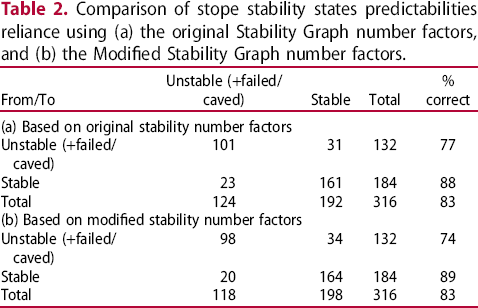
Table 2 compares the predictability reliance of stope stability states based on the use of the Original and Modified Stability Graph number factors. Based on Table 2, we conclude that there was no significant difference in the prediction capabilities using the original or modified stability number factors (Figures 7 and 9). This conclusion is supported by Figure 10.

Table 2

Comparison of stope stability states predictabilities reliance using (a) the original Stability Graph number factors, and (b) the Modified Stability Graph number factors.

From/To	Unstable (+failed/caved)	Stable	Total	% correct
(a) Based on original stability number factors
Unstable (+failed/caved)	101	31	132	77
Stable	23	161	184	88
Total	124	192	316	83
(b) Based on modified stability number factors
Unstable (+failed/caved)	98	34	132	74
Stable	20	164	184	89
Total	118	198	316	83

The lack of a difference between the Original and Modified Stability Graph number factors could also be due to bias in the database because of a higher frequency of a particular stope surface type. For example, if hangingwalls and footwalls dominate the database in an environment where these walls are relaxed, then stress factor A will have no impact on the stability number regardless of whether old or new stability number factors are used or not. We may anticipate that for some stope backs in the same environment and frequency of occurrence, some differences must occur, as the stress factor A for stope backs must be different depending on whether the original or modified factors are used (see stress factor charts in Figures 2 and 3). We investigated the possibility of such a bias masking the difference between the original and calibrated stability graph factors in the next section.

Analysis of the RSG database with the Modified Stability Graph factors

It is important to analyse the refined extended database with the modified stability number factors to determine any bias in the contributions of the stope surface data quantities and conditions on which the RSGs, as shown in Figures 7 and 9, are based.

The basic parameters in the RSG_m database are the modified stability number, shape factor, modified Q (Q′), modified stability number (N′) factors and the types of stope surfaces (i.e. backs, hangingwalls, footwalls and endwalls). The ranges of the quantitative parameters are shown in Table 3, and the frequency of occurrence of the quantitative and qualitative factors are shown in Figure 11.

Figure 11

Statistical analysis of stability number factors and stope surface distributions in the modified stability graph database: (a) Shape factor distribution (b) Stress factor distribution (c) Joint defect factor distribution (d) Gravity factor distribution for all walls (e) Garvity factor distribution for only hangingwalls (f) Distribution of stope surfaces in the database. Images are available in colour online.

Table 3

Summary of the ranges of parameters based on the Original and Modified Stability Graph number factors in the refined Extended Stability Graph database.

Parameter	Minimum	Maximum
Extended database by Trueman and Mawdesley (2003)
Q′ value	0.01	90.0
Stability number	0.005	720
Shape factor	1.03	54.9
Refined extended database with the modified factors
Q′ value	0.25	121.5
Modified stability number	0.05	720
Shape factor	1.00	23.3

The frequency of occurrence of the values of the quantitative parameters are based on 88 stope backs, 66 stope endwalls and 162 stope footwalls and hangingwalls in the RSG database. The frequencies of occurrence of these data in Figure 11 allow the determination of whether the data is biased towards one stope surface or value for example. The characteristics observed in Figure 11(a–f), are summarised as follows:

Figure 11(a) shows that the hydraulic radii of ∼50% of the stope surfaces in the refined database varies between 5 and 9 m. Only 2.2% of all stope surfaces have hydraulic radii greater than 17 m.

Figure 11(b) shows that 76% of the values of stress factor (A) for all hangingwalls and footwalls in the refined database falls within the range of 0.9–1.0, indicating relaxed zones. This implies that the stopes are designed to have the hangingwall perpendicular to the major principal stress which is horizontal in Canada and Australia (the two major sources of the database). This may imply that in stress environments where the major principal stress is vertical rather than horizontal, the stability graph method should be used with caution. This observation also shows that the lack of difference between transition zones in Figure 10 may be the result of bias in the database towards relaxed stope surfaces.

Figure 11(c) shows that for 84% of all footwalls and hangingwalls, the distribution of the joint orientation factor (B) in the RSG database is between 0.2 and 0.4. Based on this range, the dip difference between the critical joint and stope surface varies from 0° to 40°. More than 50% of the stope backs have similar Factor B distribution.

Figure 11(d) for the gravity factor (C) distribution shows that 58.6% of footwalls and hangingwalls have dips between 80° and 90°, whereas 95% of backs dip at 0–30°. This suggests that more than half of the case histories in the refined database come from steeply dipping orebodies, a characteristic of the use open stope mining method.

The distribution of Factor C for hangingwalls is shown in Figure 11(e). The dip of more than 90% of the hangingwalls is between 60° and 90°.

Figure 11(f) shows the distribution of types of stope surfaces in the database. Based on the figure, 28% of the data are from stope backs, 52% are from hangingwalls and footwalls, and 20% are from stope endwalls.

Conclusions

The Stability Graph gained popularity as an open stope design method almost four decades ago. The Original Stability Graph proposed by Mathews et al. (1981) was based on limited data. At the time, the authors noted that while the database provided proof of concept, it was inadequate for assessment of the reliability of the method. Subsequently, the database was expanded by Potvin (1988) and the stability number factors calibrated. Since then, there have been two schools of thought. One opinion is that there is no difference between the original and modified stability number factors, and therefore the former should be used, while the second school of thought argues in favour of the modified stability number factors. This difference in opinion has created confusion in the use of the Stability Graph and in expansion of the database. As a consequence, the Modified Stability Graph by Potvin (1988) which is based on the modified stability number factors, and the ESG by Trueman and Mawdesley (2003) based on the Original Stability Graph number factors, cannot be compared because they are based on different factors. The databases, therefore, cannot be combined because of the use of different stability number adjustment factors. The extended database by Trueman and Mawdesley also contained data from other mining methods other than open stoping.

To eliminate these limitations, the ESG database was critically reviewed, cleaned, and data was reproduced using the modified stability number factors and combined with the Potvin database. The modified Stability Graph database developed by Potvin was also back analysed to convert the database back to the definitions of the Original Stability Graph factors. This exercise resulted in two databases: Appendices 1 and 2 with the former based on the Original Stability Graph number factors, while the latter was based on the modified Stability Graph number factors. As a result of combining the Extended Mathews stability graph and the Modified Mathews Stability Graph databases (after data cleaning), the databases in Appendices 1 and 2 contained 316 case histories each, of which 184 stope surfaces were stable, 69 were unstable and 63 were failed.

Using the refined database with the Original Stability Graph number factors (Appendix 1) and logistic regression, the RSG_o with new stope stability state boundaries was produced and compared with the ESG_o boundaries. The comparison showed marked difference between stope stability state boundaries that could only be explained by the incorrect data used in the ESG_o development or the database size (483 versus 316 data points).

Considering that the modified stability number factors are more statistically reliable because of the database size used in their development, the Original Stability Graph number factors in the refined database were converted to the Modified Stability Graph number factors. Using the refined database with the modified factors (Appendix 2) and logistic regression, the RSG_m based on the modified stability number factors was generated.

For comparison purposes, the transition lines of the RSG_o based on the original factors were superimposed on RSG_m with the stope stability state boundaries determined from the database with the Modified Stability Graph number factors. The results indicate non-significant difference between the Original and Modified Stability Graph number factors.

Comparison between the Stability Graph variations (Figure 8) indicates that the transition lines are affected by the database size and quality rather than the stability number adjustment factors. This observation is supported by the difference in stope stability state boundaries shown in Figure 5(a,b). This observation is significant and explains that differences between the boundaries of the two graphs in Figure 5 are due to the number of case histories rather than differences between the Orginal and Modified Stability Graph number factors.

The revision of the ESG database, conversion between the original and modified stability number factors, and application of logistic regression methods have enabled the establishment of a consistent database comprising data from both the extended and modified stability graph databases for future applications.

The authors suggest caution that the conclusion that there is no significant difference between the Original and Modified Stability Graph factors may be due to the fact that the databases were bias towards relaxed surfaces, a condition that could mask the impact of high stress stope surfaces, for example, from causing a difference between the Original and Modified Stability Graph number factors.

Footnotes

Disclosure statement

No potential conflict of interest was reported by the author(s).

ORCID

F. T. Suorineni

References

AddinSoft , XLSTAT. 2019. https://www.xlstat.com/en/ .

Barton

, Lien

, Lunde

1974. Engineering classification of rock masses for the design of tunnel support. Rock Mech. 6:188–236. doi: 10.1007/BF01239496

Bawden

, Nantel

, Sprott

1989. Practical rock engineering in the optimization of stope dimensions-application and cost-effectiveness. CIM Bull. 82(926):63–70.

Clark

, Pakalnis

1997. An empirical design approach for estimating unplanned dilution from open stope hangingwalls and footwalls. Proceedings of the 99th Annual General Meeting. Vancouver: Canadian Institute of Mining, Metallurgy and Petroleum.

DeMaris

1992. Logit modeling: Practical applications. Newbury Park, USA: Sage.

Diederichs

, Hutchinson

, Kaiser

PK.

1999. Cablebolt layouts using the modified stability graph. CIM Bull. 92:81–86.

Laubscher

DH.

1994. Cave mining-the state of the art. The South African Institute of Mining and Metallurgy. p. 279–292.

Mathews

, Hoek

, Wyllie

, Stewart

SBV.

1981. Prediction of stable excavation spans at depths below 1000 m in hard rock mines. CANMET Report, DSS Serial No. OSQ80-00081.

Nickson

SD.

1992. Cable support guidelines for underground hard rock mine operations [MSc thesis]. University of British Columbia, Vancouver.

10.

Papaioanou

, Suorineni

FT.

2016. Development of a generalized dilution-based stability graph for open stope design. Min Technol. 125(2):121–128. doi: 10.1080/14749009.2015.1131940

11.

Potvin

1988. Empirical open stope design in Canada [PhD Thesis]. University of British Columbia, Vancouver.

12.

Potvin

2014. The modified stability graph method; more than 30 years later. Vol. 1, 10p. Lima, Peru: ISRM.

13.

Stewart

SBV

, Forsyth

WW.

1995. The Mathew's method for open stope design. CIM Bull. 88(992):45–53.

14.

Suorineni

FT.

2010. The stability graph after three decades in use: experiences and the way forward. Int J Min Reclam Environ. 24(4):307–339. doi: 10.1080/17480930.2010.501957

15.

Suorineni

FT.

2011. Letter to the editor Comments regarding the paper ‘factors influencing overbreak in the barkers orebody, Kundana gold mine: narrow vein case study’. In: Stewart

, Trueman

, Brunton

, editors. Mining technology: IMM Transactions section A Vol. 120(No 4). Leeds; p. 185–189.

16.

Trueman

, Mawdesley

2003. Predicting cave initiation and propagation. CIM Bull. 96(1071):54–59.

On the question of original versus modified stability graph factors – a critical evaluation