
Abstract
Due to the large size of open-pit mines’ long-term production scheduling (OPMPS) problem in large-scale deposits, it is challenging to solve that problem as the mixed integer linear programming (MILP) model. This study used an approach of the genetic algorithm (GA) to tackle this challenge. So, in a small hypothetical deposit, based on the blocks in the ultimate pit limit and scenarios with 2–6 phases, net present values (NPV) and computational times obtained from the GA and MILP model were compared to evaluate the GA. Also, the GA was applied to a large-scale deposit to determine the efficiency of the GA in real deposits. The maximum NPV was obtained for the four-phase scenario in the hypothetical deposit and the six-phase scenario in the large-scale deposit. Although the GA's NPV decreased slightly compared to the global optimum solution from the MILP model, the computational time was significantly reduced.
Keywords
Introduction
Production scheduling of open-pit mines is a fundamental problem in surface mine planning that begins with building a discrete representation of the deposit, known as a block model. A block model is a three-dimensional array of equal-sized units called a block. Thus, the deposit is broken down into blocks. A deposit's block model may contain thousands to millions of blocks regarding the size of the deposit. Each block has a set of characteristics, including mineral and contaminant grades, rock types, and rock density estimated using drill hole data (Espinoza et al. 2013). A block is extractable if the expected revenue from the sale of the metal in the block exceeds the processing cost. In other words, each block has an economic value representing the net profit. The blocks with positive and negative economic values are ore and waste, respectively (Kumral and Dowd 2021).
The open-pit mines’ long-term production scheduling (OPMPS) problem involves determining blocks extracted at each period of the mine life to maximize the mining operation's net present value (NPV). Also, different operational constraints must be observed when scheduling blocks. In addition, these blocks must be at the ultimate pit limit (UPL) of open-pit mines. The operational constraints are as follows: (Ramazan and Dimitrakopoulos 2004b; Samavati et al. 2017).
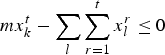
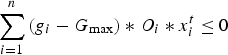
Slope constraints: All the overlying blocks that must be extracted before mining a given block must be determined. In other words, a block cannot be mined before its predecessors. Reserve constraints: A block cannot be mined more than once. Mining capacity constraints: The total amount of material (waste and ore) to be mined must be between or equal to two minimum and maximum available equipment capacities at each period. Grade blending constraints: The average material grade sent to the mill must be between or equal to two minimum and maximum grade values at each period. Processing capacity constraints: The total amount of ore cannot be more than or less than the processing capacity at each period.
The OPMPS problem has been widely studied in the last few decades due to its complexity and significant impact on the success and profitability of open-pit mine extraction projects. Solving methods for OPMPS problems can be classified into exact solution, heuristic, and metaheuristic. Exact solutions refer to techniques with a mathematical basis and ultimately find the exact answer to the problem. These methods can solve the OPMPS problem of small to medium-scaled deposits within a reasonable computational time. However, solving this problem to obtain a feasible solution for large deposits with considerable constraints may result in many decision variables, making it difficult to solve within a reasonable time. In other words, it is NP-hard, i.e. the computational time to achieve the optimal solution is not acceptable; therefore, to deal with large-scale deposits, the optimal solution is calculated approximately (Dorigo et al. 2006). As the heuristic name implies, heuristics have no mathematical basis, so the solutions obtained from these methods cannot be trusted, similar to Gershon and Wang-Sevim algorithms. Although Gershon in large block models can solve the OPMPS problem in a short time, its non-compliance with operational constraints does not provide reliable answers (Gershon 1983, 1987; Wang and Sevim 1995). Metaheuristic approaches could play a critical role in dealing with such conditions. In recent years, different researchers have tried applying these approaches to the OPMPS problem. These approaches can find the optimum or near-optimum solutions for large combinatorial problems within a reasonable time (Danish et al. 2021). The presented researches about each of these methods are stated in the following.
The MILP model, linear programming model (LP), dynamic programming, and network flow algorithm can be mentioned among the exact solutions. Gershon proposed a MILP model for mining production scheduling. However, the large number of binary variables in the OPMPS problem model makes solving it computationally tricky (Gershon 1983). In general, the number of binary variables required for the MILP model is equal to the number of blocks in the model multiplied by the total periods to be scheduled (Ramazan and Dimitrakopoulos 2004b). Elevli proposed a dynamic programming method to solve the OPMPS problem. This approach does not guarantee the solution's optimality, and its application to large-scale problems is unclear (Elevli 1995; Osanloo et al. 2008). Caccetta and Hill used the branch and cut algorithm to solve the OPMPS problem's integer programming (IP) model. This approach can produce optimal results for medium-sized problems. However, it is computationally complex for large-size problems to produce optimal results (Caccetta and Hill 2003). Ramazan proposed a mixed integer programming (MIP) scheduling model for the OPMPS problem that reduces the number of binary variables. In this case, the variables representing only the ore blocks are defined as binary, and the remaining variables are defined linearly. This method reduces the solution time and increases efficiency. Also, Ramazan introduced a block aggregation technique named a fundamental tree algorithm to reduce the number of binary variables for large-scale deposits (Ramazan and Dimitrakopoulos 2004b; Ramazan et al. 2005; Ramazan 2007). Askari-Nasab et al. proposed a MILP model to solve the OPMPS problem. To reduce the number of binary variables in the model, they grouped the blocks into larger units using fuzzy logic clustering called mining cuts (Askari-Nasab et al. 2010). In another research, Askari-Nasab et al. examined the shortcomings of the current MILP models used for the OPMPS problem, particularly the inability to solve large-scale extraction problems. This method aggregates blocks in clusters based on attributes, e.g. rock type, grade distribution, and location, to reduce the number of binary variables (Askari-Nasab et al. 2011). Gholamnejad et al. presented an integer linear programming (ILP) formulation for solving the OPMPS problem that reduces the number of active benches in any scheduling period to reduce mining equipment movement between benches in a single scheduling period (Gholamnejad et al. 2020).
As mentioned earlier, most methods can handle either a simplified version of the OPMPS problem or small to medium-scale deposits within a sufficient implementation time. However, solving this problem to obtain a feasible solution for medium to large deposits with considerable constraints may result in many decision variables, making it difficult to solve within an acceptable time. Therefore, metaheuristics could be helpful and practical in dealing with such conditions. These techniques can find the optimum or near-optimum solution to NP-hard problems within a reasonable time. In recent years, different researchers have tried applying these approaches to the OPMPS problem.
The Genetic algorithm (GA), Simulated Annealing (SA), Tabu Search (TS), and Ant Colony algorithm can be mentioned among the metaheuristic techniques. Denby and Schofield were the first to use GA because of its robustness and speed for scheduling open-pit mine production. This method used a three-dimensional block model of a copper–gold deposit that included each block's grade and rock type information, and then slope constraints were added to the problem. Among the advantages of the GA designed for an optimization problem is that it can usually be applied on a similar problem with little or no change, and often in less than 10 generations, a near-optimal solution for some problem types is found (Denby and Schofield 1994). Alipour et al. introduced a GA-based approach to the OPMPS problem. This approach randomly generated the initial population and ensured each solution's feasibility through a normalization function. However, grade-blending constraints were not considered (Alipour et al. 2020, 2022). Kumral and Dowd were the first to use SA to solve the OPMPS problem. The Lagrangian parameterization technique obtained the initial sub-optimal solution for multi-objective SA optimization in this technique (Kumral and Dowd 2005). Lamghari and Dimitrakopoulos, to solve the OPMPS problem, used TS and variable neighbourhood descent algorithms. This approach could produce a near-optimal solution in a reasonable implementation time (Lamghari and Dimitrakopoulos 2012). Shishvan and Sattarvand applied the Ant Colony algorithm for the open-pit mine production planning problem (Shishvan and Sattarvand 2015). Finally, Khan & Niemann- Delius utilized particle swarm optimization and differential evolution to solve the open-pit mine production planning problem (Khan and Niemann-Delius 2014, 2018).
By studying different production scheduling methods, three approaches can be used to solve the OPMPS problem based on the phases created within the UPL of open pit mines. The first approach extracts the most valuable phase in the first period. In this approach, phases are divided from top to bottom. The blocks related to the selected phase are removed, and then this process is repeated for all the remained blocks in the UPL. In other words, maximizing the NPV of a mining project is achieved with high-grade ore extraction as soon as possible. Therefore, when phases are used to find the optimum production schedule, these phases should be maximum-metal phases for the resulting schedule to be optimum. A maximum-metal phase of size N is a phase that contains more metal than any other phase of the same size N. Gershon used this approach to OPMPS (Gershon 1987; Wang and Sevim 1995).
The second approach divides phases from the bottom of the UPL upwards. In this approach, the least valuable phase, or the phase with the lowest grade, is extracted in the last period. The blocks related to the selected phase are removed, and then this process is repeated in the entire area of the UPL for the remaining blocks. Wang and Sevim used this approach to the OPMPS problem (Wang and Sevim 1995).
Finally, in the third approach, all of the UPL is decided simultaneously based on NPV.
The third approach can find the optimal solution. Exact methods such as the mixed integer linear programming (MILP) model use this approach to solve the production scheduling problem. However, solving the production scheduling problem in open pit mines with this approach in large-scale deposits becomes an NP-hard problem. Generally, using the second approach leads to having maximum NPV compared to the first. Therefore, in larger-scale deposits where the MILP model cannot solve the OPMPS problem, the second approach can help solve the problem.
In the studies accomplished to solve the OPMPS problem, among the three mentioned approaches, the third approach has been used in some of the exact solutions. However, other approaches have rarely been used. Also, among the studies performed using GA to solve the OPMPS problem, the shape of the pits is changed by mutation and crossover operators. In this case, reserve and slope constraints are not satisfied. Therefore, it needs a normalization step.
Nevertheless, normalization is unnecessary when the first and second approaches are used. Instead, the slope and mining capacity constraints are applied from the beginning in this approach to the problem. Therefore, this reduces the complexity of the problem. In this paper, GA is used as the second approach to solving the OPMPS problem, and all operational constraints have been applied on the studied problem.
Genetic algorithm
Most metaheuristic algorithms are inspired by the biological evolution process, swarm behaviour, and physics law. In general, these algorithms are categorized into single-solution and population-based metaheuristic algorithms. The population-based metaheuristic uses several candidate solutions during the search process. These metaheuristics maintain the variety in the population and avoid the solutions being stuck in local optima. One of the well-known population-based metaheuristic algorithms is GA, inspired by the biological evolution process. GAs perform searches in complex and large problems and provide near-optimal solutions for an optimization problem's objective or fitness function (Maulik and Bandyopadhyay 2000; Katoch et al. 2021).
GA is a population-based search algorithm that utilizes the concept of survival of the fittest. In this algorithm, the population is the solution space that includes chromosomes, which is considered an advantage of the GA because it provides a wide range of suitable solutions (chromosomes). Each chromosome consists of several genes. Also, all possible solutions must be developed to achieve the best solution (Katoch et al. 2021; Alipour et al. 2022). After calculating the fitness of each solution, which has different methods based on the type of problem, a method such as the roulette wheel is used to select a new population based on the calculated fitness (Pencheva et al. 2009). Then, crossover and mutation operators are applied to chromosomes.
Single-point crossover is the most approved crossover, which is widely in use. This way, a crossover site is randomly selected along the length of two chromosomes, and genes next to the cross-sites are interchanged. In this case, when a suitable location is chosen, better progeny can be obtained by combining the good qualities of the parents. As a challenging issue, using the crossover alone to create a child causes the GA to get stuck in the local optimal. So, the mutation is used to reduce this problem by proving the difference between new children and parents and encouraging diversity. One type of mutation is the flip-bit mutation that reverses the value of a randomly selected gene (Pencheva et al. 2009; Omar and Hirotaka 2012; Kora and Yadlapalli 2017). The process of evolution is repeated until the final condition for obtaining the chromosome with the best fitness value is met; this is known as the termination criteria (Maulik and Bandyopadhyay 2000; Hassanat et al. 2019). Since the GA is a flexible method, the results can be improved by changing its parameters. In other words, in the OPMPS problem, by performing sensitivity analysis on a number of its parameters, the NPV presented by the GA is checked, and the best value is selected (Ataei M and Osanloo M 2004; Villalba M et al. 2019). Therefore, chromosome representation, fitness function computation, crossover, mutation, and selection are the critical elements of GA. In this study, Single-point crossover and flip-bit mutation are used.
Open-pit mine production scheduling problem
OPMPS problem specifies a block mining sequence to maximize the NPV under mining and processing capacity and grade blending constraints, in addition to the slope and precedence constraints. These constraints and the methods to solve the problem will be explained in the following.
Open-pit mine production scheduling using MILP
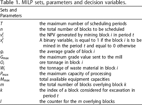
MILP sets, parameters and decision variables.
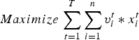
The objective function:

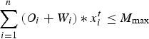
Processing capacity constraints:
Genetic Algorithm for long-term open-pit mine production scheduling
This section examines how to create the objective function, generate the chromosome, select the new population, and determine the parameters related to the GA in the studied problem.
The objective function generation
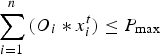
The objective function of the OPMPS problem in this study is a function of the number of ‘candidate blocks.’ Candidate blocks are selected from downward cones that accept the mining capacity constraints. A downward cone is a cone created for each block subject to slope constraints. This cone should be limited to UPL. The highest block of each cone is the apex block. That is until that block is not extracted, blocks inside the cone cannot be mined. In this research, downward cones are utilized to employ the second approach. For example, Figure 1 shows a UPL of a hypothetical two-dimensional block model in which an upward cone is made for block A and a downward cone for block B.
The concept of upward and downward cones in the 2D UPL model.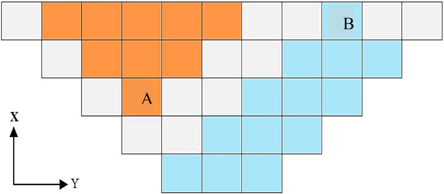
Defining a specific capacity for downward cones is necessary to comply with the mining capacity constraints. In this study, the capacity is defined based on the number of blocks inside each downward cone. Accordingly, if the number of blocks inside the downward cone corresponding to each block is proportional to the defined capacity, it is called a candidate block. A candidate block is a block that has the ability and conditions to be separated from the UPL in the last period. This mean is if a downward extraction cone is made for this block, the number of blocks located in this cone should be smaller or equal to the number of blocks in the current phase.
For a better understanding of the matter, a hypothetical two-dimensional UPL is considered in Figure 2. The capacity of the last extraction phase is considered in four blocks. In this case, the block with the number 6 is not a candidate block because the number of blocks in the downward extraction cone of this block is five, which is more than the current phase mining capacity (Figure 2(a)). In addition, the block with the number 11 is a candidate block because the number of blocks located in the downward extraction cone of this block is three blocks, which is less than the desired number of blocks in the current phase (Figure 2(b)). All candidate blocks within the UPL are shown in Figure 2(c).
A hypothetical two-dimensional UPL, a: not a candidate block, b: a candidate block, c: all the candidate blocks in UPL.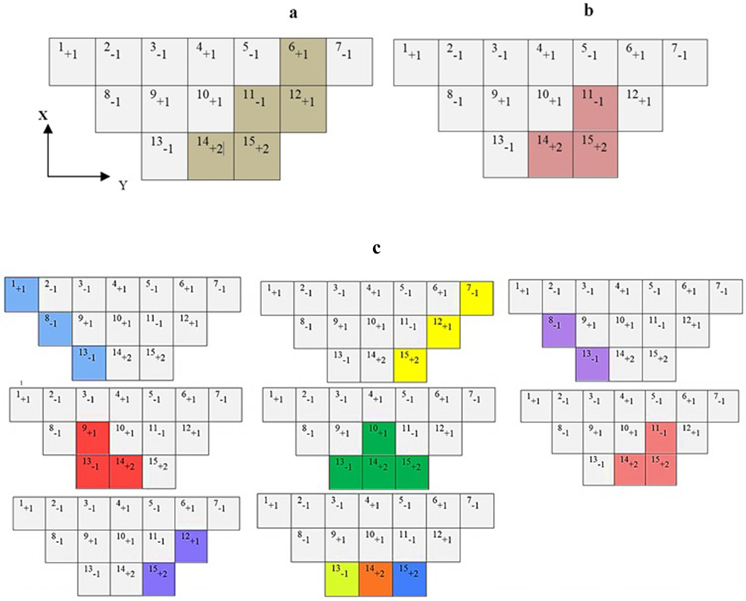
In each step for all the blocks in the UPL (or the remaining blocks after extracted previous phase blocks), a downward cone is made; if that block is a candidate block, it can be placed in the search space of the genetic algorithm for the current period.
The chromosome generation
After generating the objective function, some random initial solutions (chromosomes) based on the population size are defined. The population size depends on the nature of the problem but typically contains 50–100 possible solutions (Mirzaei-Nasirabad and Khalokakaie 2008). In this research, the population size is considered to be 90.
The length of the chromosomes (initial solutions) equals the number of columns (the blocks in the block model in tandem layers with the same X and Y directions) with at least a candidate block. Each gene state is based on the number of candidate blocks in each column corresponding to that gene. So, the initial population is randomly made based on this number of states. For better understanding, in Figure 2(c), there are seven columns of blocks with at least a candidate block. Therefore, the chromosome length is equal to seven. For example, column 4 has two candidate blocks (block numbers 10 and 14). Therefore, the number of states this column creates in the chromosome is three. That means it can extract this column candidate blocks in three situations. (1) Mode zero: extracted no block. (2) Mode 1: extracted the cone corresponding to the candidate block with the number 14. (3) Mode 2: extracted the cone corresponding to the candidate block with the number 10. Finally, based on these states, three different chromosomes can be generated.
Apply the operational constraints
After creating the initial population, the fitness value of the chromosomes is calculated. Operational constraints related to solving the OPMPS problem should be applied to calculate this value. In this case, the processing capacity constraints and grade blending constraints can be applied by penalizing the fitness values of the chromosomes that do not meet each of these constraints or rewarding the fitness values of each. In this study, to effectively implement the mentioned constraints, a combination of both modes was used. Slope, reserve, and mining capacity constraints are satisfied by making downward cones for every selected candidate block. Then, a roulette wheel is used to select a new population. In this wheel, a random number is generated according to each chromosome. Therefore, a new individual is created based on the value of that number and each chromosome's fitness function.
Apply the GA parameters
In the next step, crossover and mutation operators are applied on the population after applying mentioned constraints on chromosome fitness. Therefore, single-point crossover and flip-bit mutation were used to solve the OPMPS problem with GA. Crossover and mutation were also selected from intervals [0.3,0.5] and [0.05,0.15], respectively (Mirzaei-Nasirabad and Khalokakaie 2008). The goal is to reach the maximum NPV during the life of the mine in the shortest time possible. Then, the fitness value of the chromosomes is calculated again, and the chromosome with the lowest fitness value is picked in the lowest phase. In other words, in the selection step, the chromosome with the lowest fitness is determined. This process is repeated until a termination condition has been reached. The optimizing process will be terminated if the best solution does not change during m iteration. In this study, m is considered 500 iterations. Therefore, the blocks related to the designed phase are removed; Then, the algorithm is repeated for the next phase with the remaining blocks in the UPL. Finally, the algorithm continues until all the blocks within the UPL are assigned to different phases.
As mentioned before, using sensitivity analysis, the best deals are got for the parameters of the GA, namely crossover and mutation, obtained when the maximum NPV is received. The most common approach to using sensitivity analysis is changing one factor at a time to understand what effect this produces on the output. That appears logical, as any change observed in the result will unambiguously be due to the single parameter change. Furthermore, one can keep all other parameters fixed to their central or base values by changing one parameter simultaneously. This method increases the comparability of the results (all ‘effects’ are computed regarding the same central point in space) and minimizes the chances of computer program crashes, more likely when several input factors are changed simultaneously (Saltelli and Annoni 2010). Therefore, the sensitivity analysis results are checked to determine the maximum NPV and the best crossovers and mutations are determined.
The mentioned steps of the GA for solving the OPMPS problem are according to Figure 3.
Steps of the GA to solve the OPMPS problem.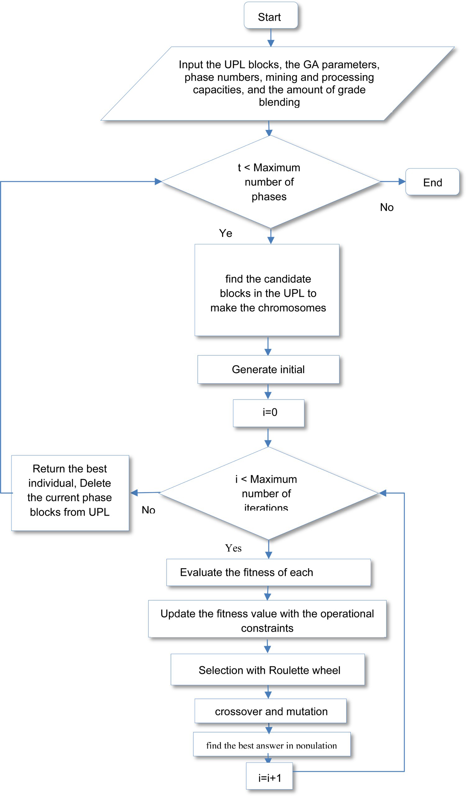
Implementations and results
In this section, to evaluate the results of solving the OPMPS problem in open pit mines by GA, this algorithm and MILP model were applied on a hypothetical deposit. Then, to determine the efficiency of GA in solving the OPMPS problem in real mines, the algorithm was also applied on a large-scale deposit. In the following, the results related to the hypothetical and the real deposits are discussed separately.
A small hypothetical deposit
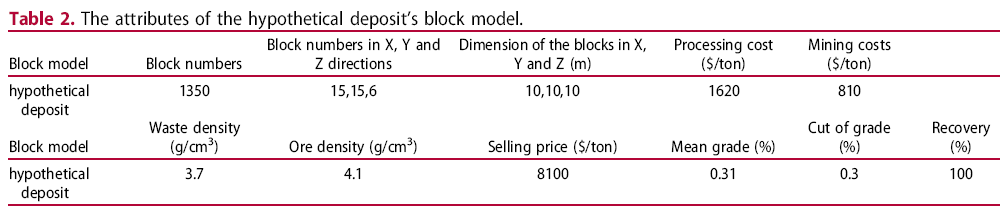
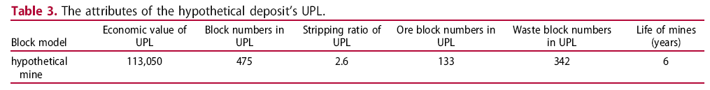
A small hypothetical deposit was used to evaluate and verify the GA results compared to the MILP because implementing the MILP on the real deposit was very time-consuming. In addition, before performing OPMPS, it is necessary to determine the UPL for the mentioned deposit. Then, the production schedule should be done for the blocks inside this area. The attributes of the deposit's block model and its UPL are given in Tables 2 and 3, respectively. Also, the grade histogram of blocks in UPL is according to Figure 4.
The UPL's blocks grade histogram of the hypothetical deposit. The attributes of the hypothetical deposit's block model. The attributes of the hypothetical deposit's UPL.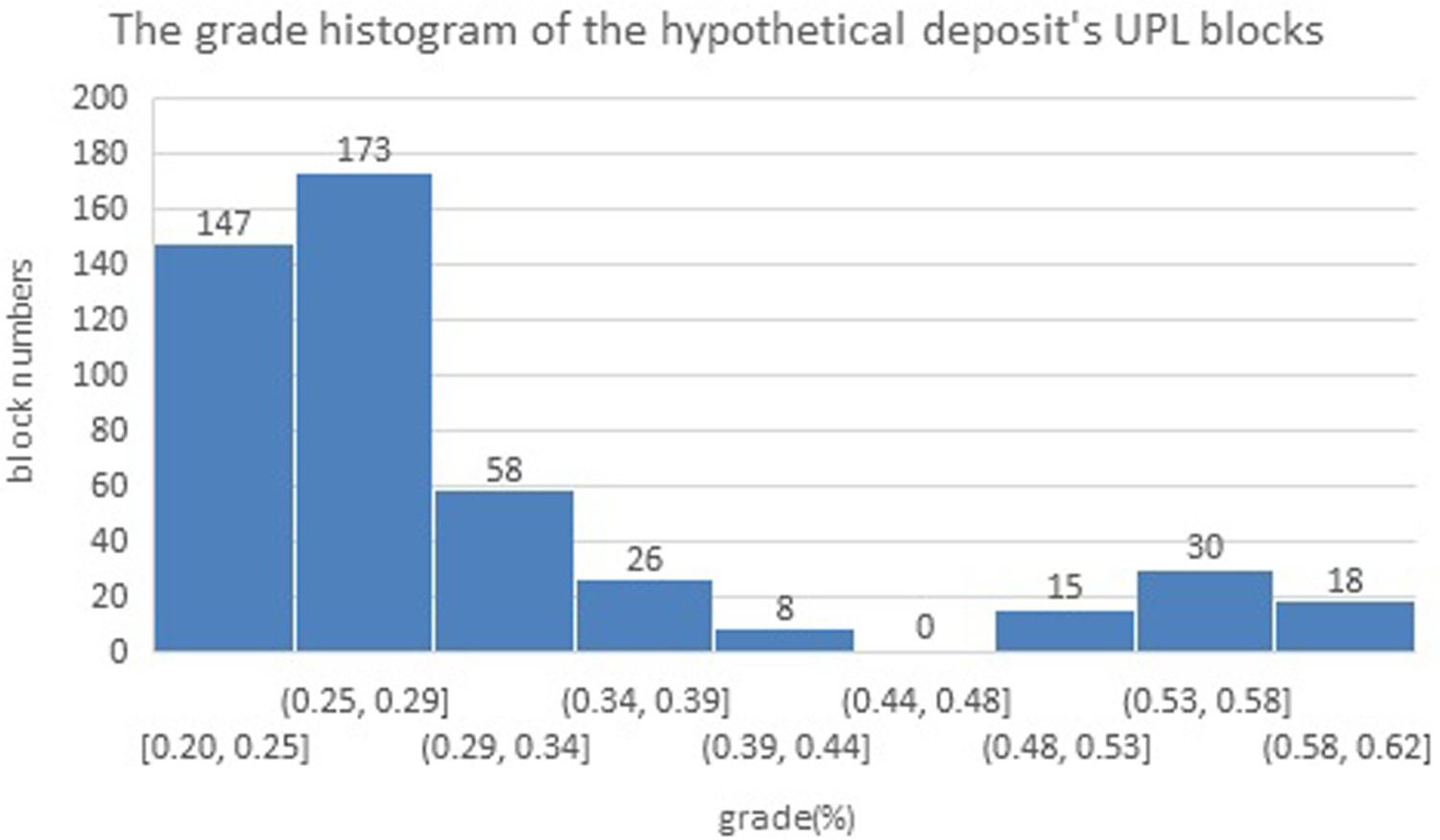
The GA and MILP were applied on the block model in different scenarios. These scenarios are based on the number of phases between 2 and 4. That is 2 phases as the first scenario, 3 phases as the second scenario, and 4 phases as the third scenario. Then the NPV obtained from each scenario is compared with the others, and the highest value is selected as the optimal state.
The study is executed in the Intel Core™i7-4702 PC (3.4 GHz) with 16 GB of RAM. The CPLEX exact solver linked to MATLAB was used to solve the problem of the current study with the MILP model.
The results of solving the OPMPS problem by MILP and GA in the hypothetical deposit.
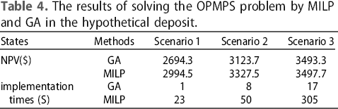
The difference in the NPV resulting from GA and MILP.
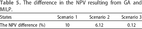
The average grade, stripping ratio, and block numbers in each scenario.
The typical cross-section of UPL for scenario 3 of GA is shown in Figure 5.
A cross-section (X = 190) view of the hypothetical deposit's UPL for scenario 3 of GA.
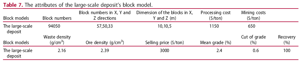
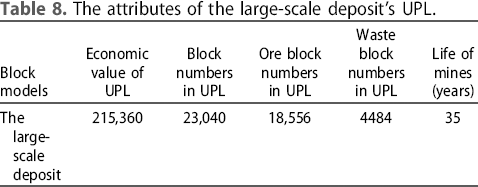
A large-scale deposit
After evaluating the GA results in solving the OPMPS problem in the small deposit, this section studies its capability on the real deposit. The attributes of the large-scale deposit's block model and its UPL are given in Tables 7 and 8, respectively. Also, the grade histogram of blocks in the UPL is according to Figure 6.
The UPL's blocks grade histogram of the large-scale deposit. The attributes of the large-scale deposit's block model. The attributes of the large-scale deposit's UPL.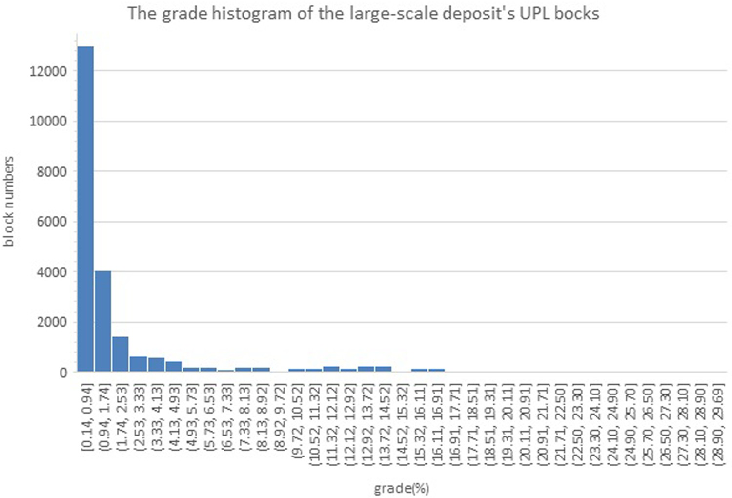
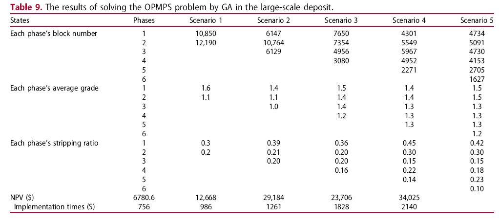
The GA was applied on the block model in five scenarios. These scenarios have 2–6 phases. Then the NPVs obtained from scenarios were compared, and the highest NPV was selected as the optimal state.
The results of solving the OPMPS problem by GA in the large-scale deposit.
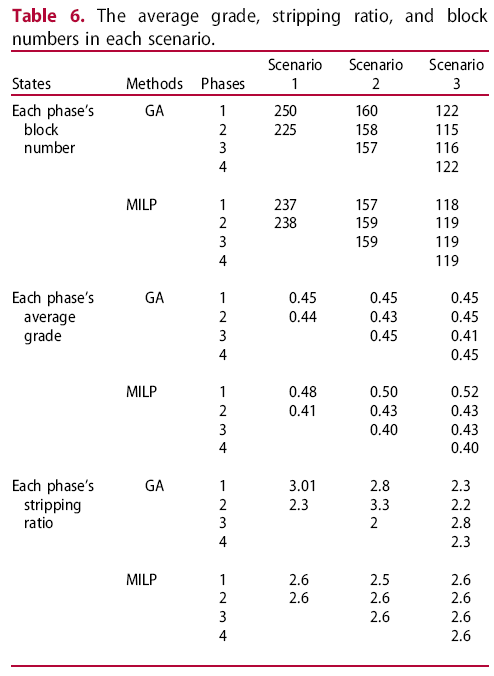
The plan view of UPL for scenario 5 at level 1610 is shown in Figure 7.
A 2D view of large-scale deposit's UPL for plan 1610.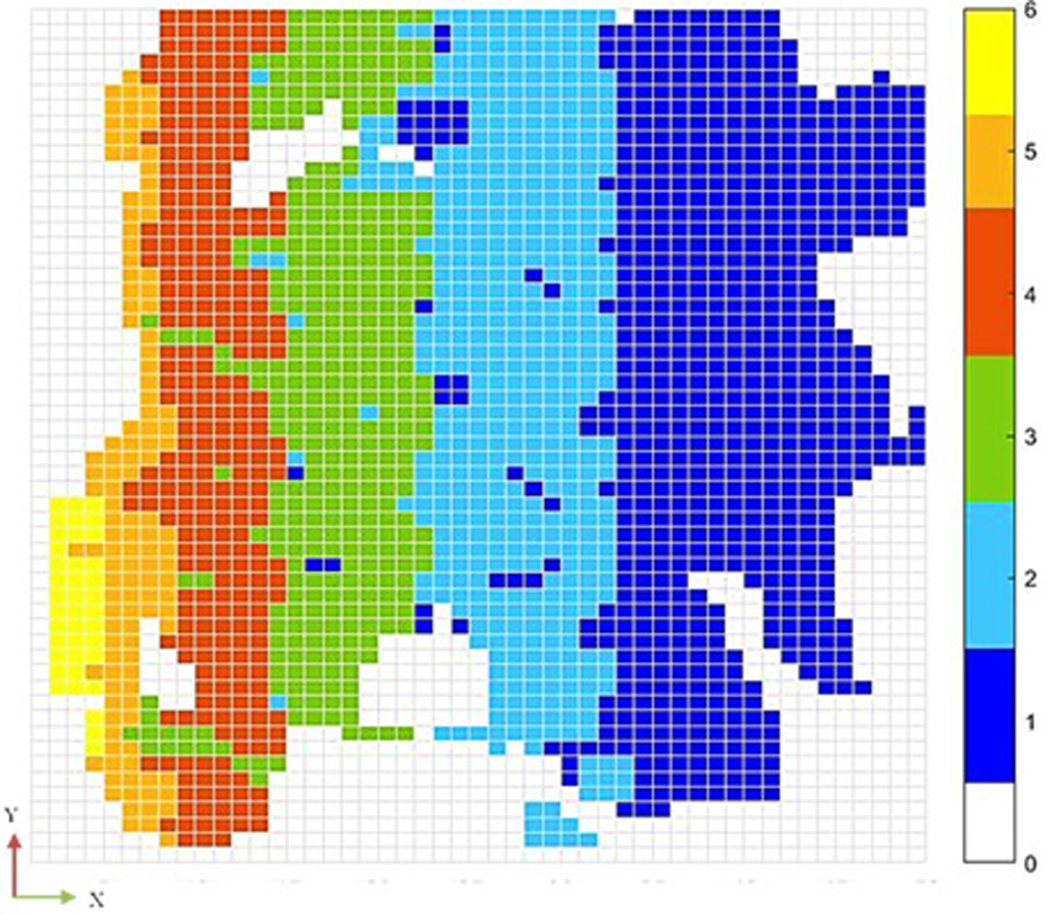
Exact solutions always provide the best answer in solving optimization problems. However, implementing these methods, similar to MILP on large-scale deposit production scheduling, is time-consuming and is increased with the increasing number of phases (Table 9). Production scheduling studies need to provide an appropriate answer in a reasonable time. Therefore, GA is proposed as a fast method with a near-optimal answer. In this case, by considering all the operational constraints, the GA can provide an appropriate answer in a shorter time than MILP. In addition, by applying sensitivity analysis, the appropriate value of its parameters similar to crossover and mutation can be adjusted to achieve the maximum NPV.
Conclusions
OPMPS problem in large-scale deposits using exact solutions such as MILP becomes an NP-hard problem. That is, it cannot be solved in a reasonable time, or it cannot be solved at all because of the many blocks followed by many binary variables. One way to solve this problem is to use metaheuristics such as GA because it performs the search in large-scale problems and provides the near-optimal solution for the OPMPS problem in less time than the MILP. The advantage of this algorithm over the other metaheuristic algorithms is that GA maintains the variety in the population and avoids the solutions being stuck in local optima.
This research aims to use GA in long-term open-pit mine production scheduling. The GA results obtained in the production scheduling of a small hypothetical deposit were compared with those obtained from MILP to evaluate the efficacy of GA. These two methods were applied on this block model in three scenarios based on the number of phases. By comparing the NPVs obtained from the two methods, it was found that the NPV obtained from the GA in the four-phase scenario is, at most, 0.12% lower than the NPV obtained from the MILP. However, it provided the answer in just 17 s, which is 288 s faster than MILP. This computation time difference in large-scale deposits may reach several days. Then, GA was applied on a real mine to determine its capability on large-scale deposits. The maximum computing time for GA in this deposit was approximately 36 min, corresponding to the six-phase scenario. This item provides the highest amount of NPV. So considering all the operational constraints, GA is proposed as a faster solution method with a near-optimal solution.
Footnotes
Disclosure statement
No potential conflict of interest was reported by the author(s).