
Abstract
Geostatistical modelling of grades in mineral deposits often requires the simulation of multiple related variables that have sum and fraction constraints. Sum constraints occur when the sum of some variables may not exceed or must equal a given constant. Fraction constraints occur when a variable may not exceed another variable. In this case, the geostatistical simulations should reproduce the histograms, variograms, multivariate relationships and honour the constraints. We present a methodology for the geostatistical simulation of multiple related variables that considers sum and fraction constraints. The methodology is illustrated in a case study. The data were obtained from a bauxite deposit. First, the original variables were re-expressed as ratios. Second, the variables were transformed using the Projection Pursuit Multivariate Transform (PPMT). Then the PPMT transformed variables were simulated independently using sequential Gaussian simulation and back-transformed. The simulations reproduced the histograms, variograms and bivariate relationships and honoured the sum and fraction constraints.
Keywords
Introduction
Geostatistical modelling of grades in mineral deposits commonly requires prediction of multivariate data with sum and fraction constraints. Sum constraint occurs when the sum of some variables must be less or equal to a constant. For instance, the sum of all grades may not be above one hundred per cent. Fraction constraint occurs when one variable is a fraction of the other. For example, in a bauxite deposit, the recoverable alumina is a fraction of the total alumina. As a result, the recoverable alumina may not exceed the total alumina within any grid node of the simulated model. Multivariate geostatistical simulations should honour these constraints.
Most geostatistical simulation algorithms rely on the multivariate Gaussian distribution assumption. The Projection Pursuit Multivariate Transform (PPMT) (Barnett et al. 2014, 2016) transforms the data into variables that are uncorrelated and follow a multivariate Gaussian distribution. Then, the geostatistical simulation techniques may be applied to these transformed variables individually without the need for cokriging or the linear model of coregionalisation (Journel and Huijbregts 1978) to reproduce possible cross-correlations among them. The PPMT reproduces well the multivariate relationships between the data (Barnett et al. 2014, 2016; Manchuk et al. 2017). However, PPMT does not explicitly consider sum and fraction constraints.
One method to deal with variables that have sum constraint is based on using ratios or log-ratios of the original variables (Pawlowsky-Glahn and Olea 2004; Pawlowsky-Glahn and Egozcue 2006; Barnett and Deutsch 2012; Boisvert et al. 2013; Mery et al. 2017). This approach has been used successfully with compositional data. Compositional data represent a set of variables that sum to a constant. When the data does not sum to a constant, a filler variable may be added to the data set. The filler variable corresponds to the constant minus the sum of the remaining variables. The most common transformations for compositional data are the additive log-ratio (Aitchison 1986), centred log-ratio (Aitchison 1986) and isometric log-ratio (Egozcue et al. 2003). Manchuk et al. (2017) used the isometric log-ratio followed by PPMT to account for the sum constraint of the data set. In this paper, we used a ratio similar to the additive log-ratio. The difference is that the logarithmic was not calculated.
To deal with fraction constraints, Emery (2012) and Hosseini and Asghari (2015) used the stepwise conditional transformation (Leuangthong and Deutsch 2003) to transform the data into Gaussian values before geostatistical simulation. The simulations honoured the fraction constraint. The drawback is that the stepwise conditional transformation requires a large number of data when dealing with many variables. The case studies showed by Emery (2012) and Hosseini and Asghari (2015) considered only two variables. We propose, instead of simulating the total and fractional grade, simulating the total grade and the ratio of the fractional grade divided by the total grade, which is called fraction ratio. The simulated fractional grade is obtained by multiplying the simulated fraction ratio by the simulated total grade.
The multivariate geostatistical simulation case studies found in the literature deal with either a sum constraint (Barnett and Deutsch 2012; Boisvert et al. 2013; Mery et al. 2017) or a fraction constraint (Emery 2012; Hosseini and Asghari 2015). In this paper, we present a case study of multivariate geostatistical simulation that contains both sum and fraction constraints. The data set contains seven variables and was obtained from a bauxite deposit in Brazil.
Methods
This section provides details of the transformations used in the case study.
Ratio for sum constraint
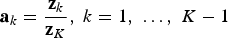
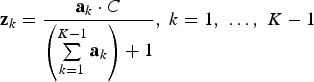
The ratio used here is similar to the additive log-ratio (Aitchison 1986), but it does not calculate the logarithm. The ratio is denoted in this paper as ratios A. Suppose variables whose sum is equal to a constant C. If the sum of the variables is not equal to a constant, a filler variable may be added. A filler variable is obtained as the constant C minus the sum of the remaining variables. Equation (1) describes the ratios A:
 is the new variable to be modelled, and
 is the original variable. Equation (2) describes the inverse of ratios A:
Note that the last grade
 is C minus the sum of the K−1 others.
Ratio for fraction constraint
We denote the total grade as
 and the fractional grade as
 . The fraction ratio
 of these grades is obtained by Equation (3):

The simulations are performed using the variables
 and
and
 . Then the simulations of
 are obtained by multiplying the simulations of
 by the simulations of
 .
.
Projection pursuit multivariate transformation
The PPMT (Barnett et al. 2016; Manchuk et al. 2017) involves the following steps:
Normal score the variables; Sphere transform the variables; Find an interesting projection of the data; Normal score the data along the projection found in step iii; Repeat steps (3) and (4) until the data is multivariate Gaussian with an identity covariance matrix.
Normal score transformation
The normal score transformation (Deutsch and Journel 1998) changes a variable so that the transformed variable has a univariate standard Gaussian distribution. Consider the data matrix
 with
with
 data vectors
 . The normal score transformation consists of matching the quantiles of the cumulative distribution function (cdf) of the original data
 with the standard Gaussian cdf
 (Equation (4)):
 is the vector of the transformed data. The application of the normal score transformation to all the vectors of the data matrix
 results in the transformed data matrix
 . Equation (5) defines the normal score back-transformation:
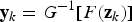
Data sphering
Consider the normal score data
 . Data sphering of
 consists of the following operation (Equation (6)):

 is obtained with the following matrix multiplication (Equation (7)):
 and
and
 are the eigenvalue and eigenvector matrixes obtained from the spectral decomposition of the covariance matrix
 (Equation (8)):
Sphering can be understood as rotating the normal score variable units to principal components, standardising the variance of each principal component, and then rotating the scaled principal components back to the normal score variable axes. The sphered variables are univariate Gaussian and uncorrelated, but complex multivariate relationships are still present in the data.
Projection
The projection
 of the data matrix
 into a unit vector
 is defined as a matrix multiplication (Equation (9)):

The interesting projections are the most non-Gaussian projections. The PPMT uses a projection index
 to measure the non-Gaussianity of a projection (Barnett et al. 2016). An optimised search is used to find the projections that maximise
 . After the most non-Gaussian projection is found, the normal score transform is applied to the projection. The process is repeated until the data follow a multi-Gaussian distribution and are independent. The stopping criterion is based on bootstrap sampling (Barnett et al. 2014). First, a series of multivariate Gaussian distributions with identity covariance matrix is generated. Then the index
 is calculated for a number of orientations, which results in a distribution of projection indices
 . The user specifies the percentile of
 that should be reached by the projection index
 calculated with the transformed data. In addition, the user specifies a maximum of iterations in case the percentile is not reached.
Case study
Data set presentation and declustering
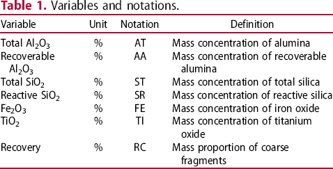
Variables and notations.
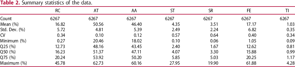
Summary statistics of the data.
The coefficients of correlation between the variables are shown in Figure 1. The fractional grades AA and SR have high correlation with the corresponding total grades (AT and ST), as expected.
Correlation matrix of the data.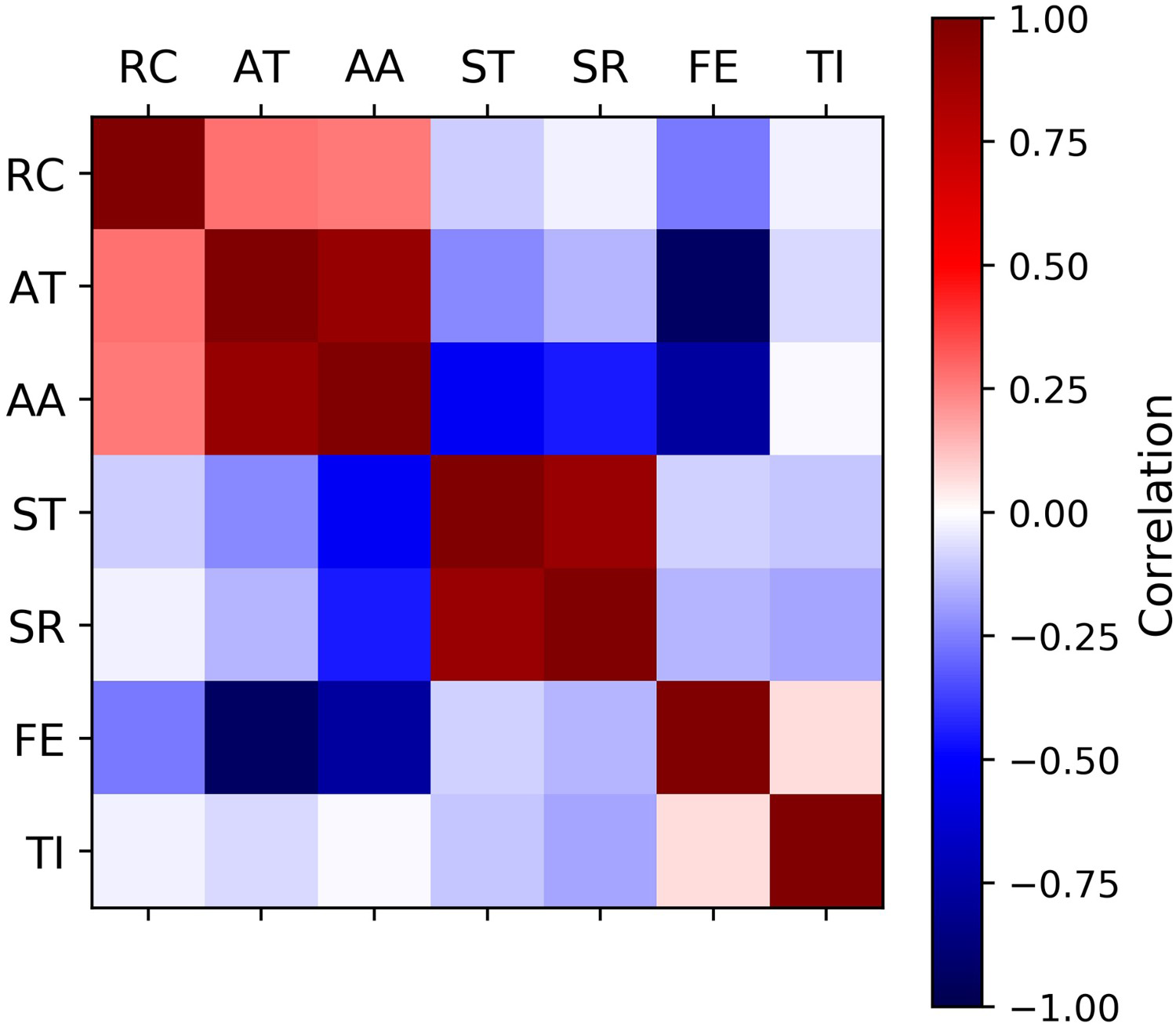
The data have an irregular sampling spacing (Figure 2). The sparsest sampling spacing is roughly 200 × 200 m along the X and Y directions while the densest sampling spacing is about 25 × 25 m along the X and Y directions. Furthermore, the area contains intermediate sampling spacings of 100 × 100 m and 50 × 50 m along the X and Y directions. The samples were obtained from vertical drill holes, and the sampling length is at every 0.5 m. The original Z coordinates were transformed into stratigraphic coordinates. The stratigraphic coordinate corresponds to the distance relative to the top of the bauxite seam.
Location map of the samples.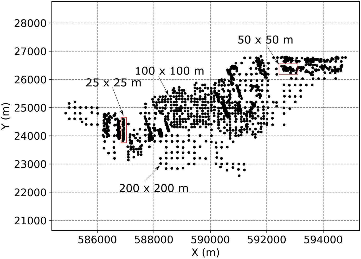
Cell declustering (Deutsch and Journel 1998) was performed in two dimensions. Pyrcz and Deutsch (2014) recommend performing cell declustering in two dimensions when the drill holes are vertical and fully intersect the formation. The cell size is 200 m along the X and Y directions and corresponds to the sampling spacing in the sparsely sampled areas.
Methodology
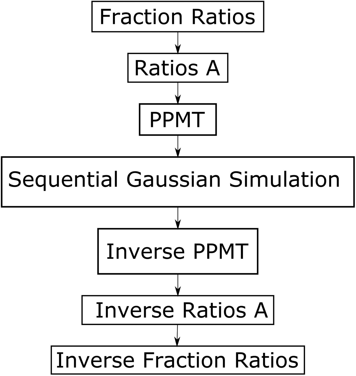
The flowchart of the methodology is shown in Figure 3. First, the fractional grades AA and SR were transformed into fraction ratios (Equation (10)):
Flowchart of the methodology.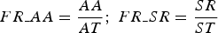


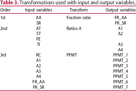
Third, PPMT was applied to the ratios A, the fraction ratios and RC. The histogram and scatter plot of the first two PPMT transformed variables are shown in Figure 4. The variables have a Gaussian distribution and are independent, with zero correlation (Figure 4). A summary of the transformations with the input and output variables is shown in Table 3.
Histogram and scatter plot of the first two PPMT transformed variables. Transformations used with input and output variables.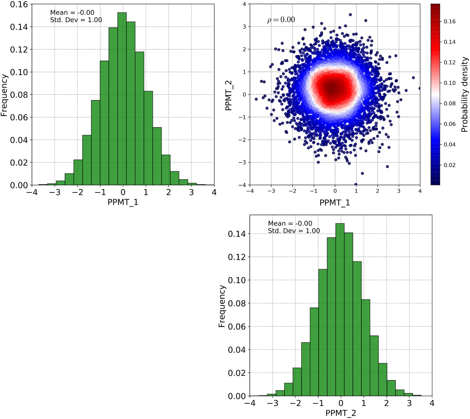
The transformed PPMT variables were simulated using sequential Gaussian simulation (SGS). We generated 50 realisations. The simulated PPMT variables were back-transformed to original units. First, the PPMT back-transformation was applied to obtain the simulation of RC, A1, A2, A3, A4, FR_AA and FR_SR. Next, the inverse of ratios A was used to transform the variables A1, A2, A3 and A4 into AT, ST, FE and TI. Last, the simulations of AT and ST were multiplied by the simulations of FR_AA and FR_SR to obtain the simulations of AA and SR. The first realisation of RC, AT and ST is shown in Figure 5.
First realisation of RC (top), AT (middle) and ST (bottom). The vertical exaggeration is 80:1.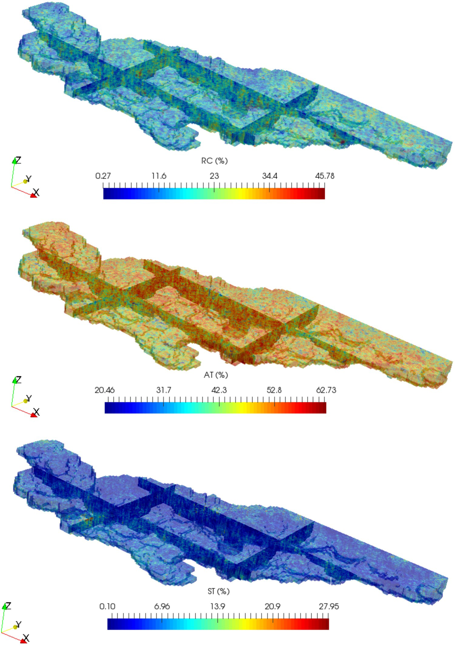
Variogram analysis
Variogram models used in the simulations.
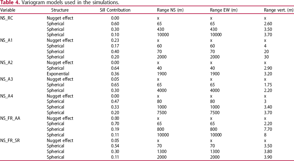
The experimental variograms were calculated using stratigraphic coordinates. The nugget effect was fitted based on the vertical experimental variogram. The sill of the variograms was fitted to one, and the ranges along the horizontal plane were fitted according to the experimental variograms in the horizontal plane.
Results and discussion
Histogram reproduction
The histogram of the realisations was compared with the histogram of the declustered data (Figure 6). Overall, the simulations reproduce the histograms of the original variables. The mean and standard deviation of the realisations are close to the mean and variance of the declustered data.
Comparison between the histogram of the realisations and the declustered data.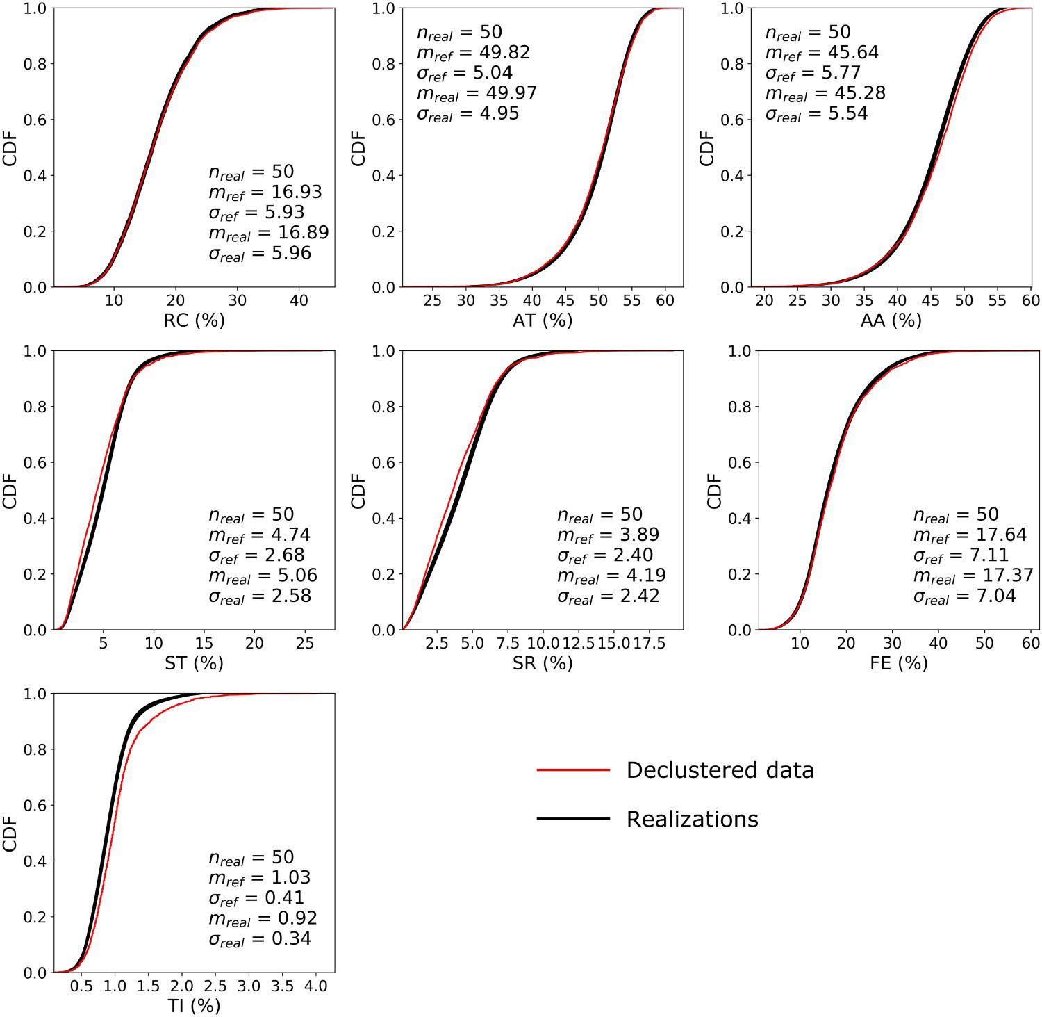
Variogram reproduction
The variograms of the data and realisations along the horizontal direction were compared (Figure 7). RC and TI had a good reproduction of the variogram for the short and long-range structures. For the variables AT, AA, ST, ST and FR, the variogram of the realisations reached a sill greater than the sill observed in the variogram of the data. This is likely due to the nonstationary nature of the variables, that is, there is a zonal anisotropy in the horizontal plane perpendicular to the stratigraphic coordinate.
Variograms of the realisations and the data along the horizontal direction.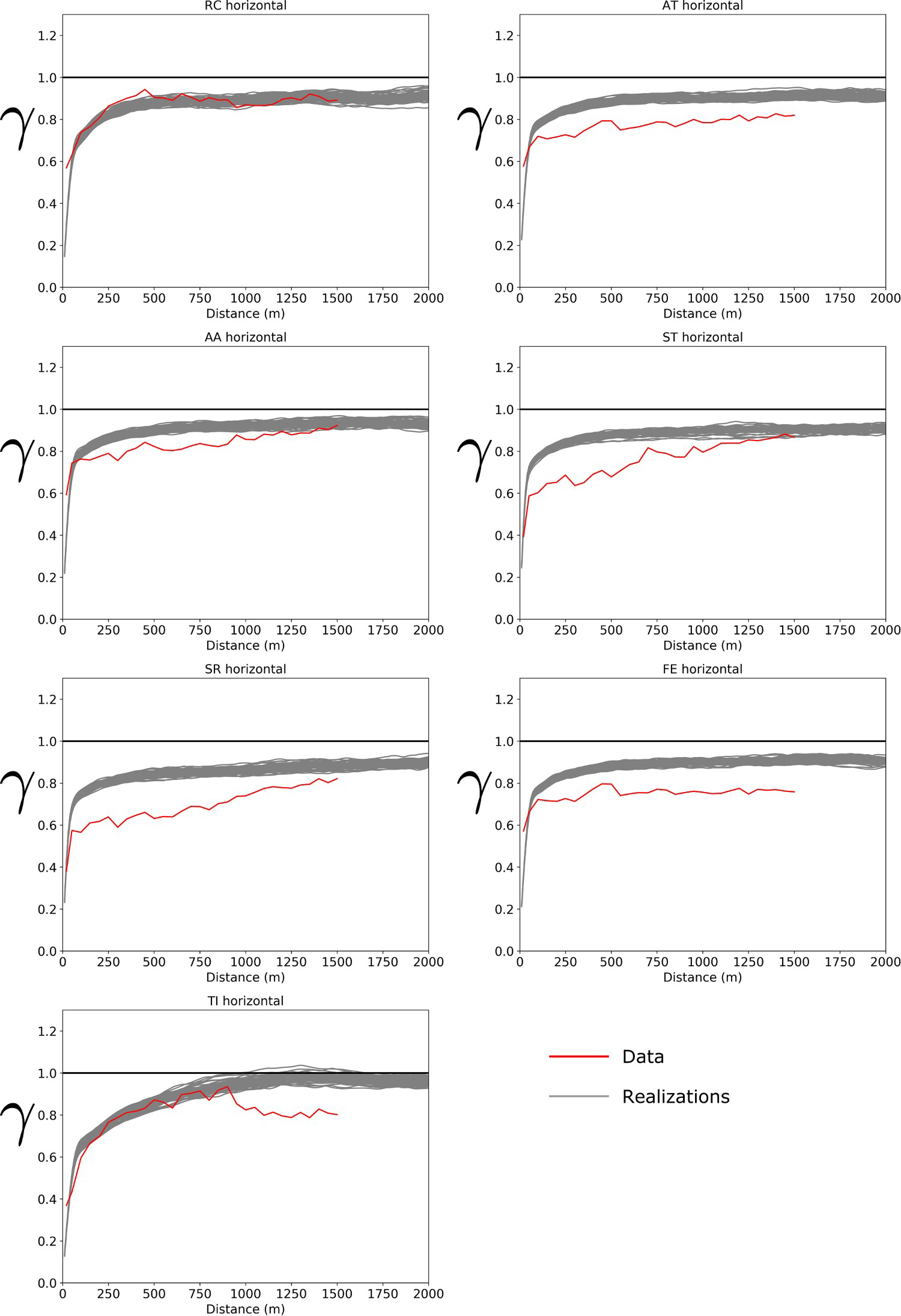
The variograms of the data and realisations along the vertical direction were compared (Figure 8). Overall, the variograms of the realisations are similar to the variograms of the data. The worst variogram reproduction occurred for the variables AT and FE, whose realisations are more spatially continuous than the data. The variograms of some variables indicate a vertical trend, as they increase above the sill. We assumed that the vertical trend was enforced in the simulation by the conditioning data.
Variograms of the realisations and the data along the vertical direction.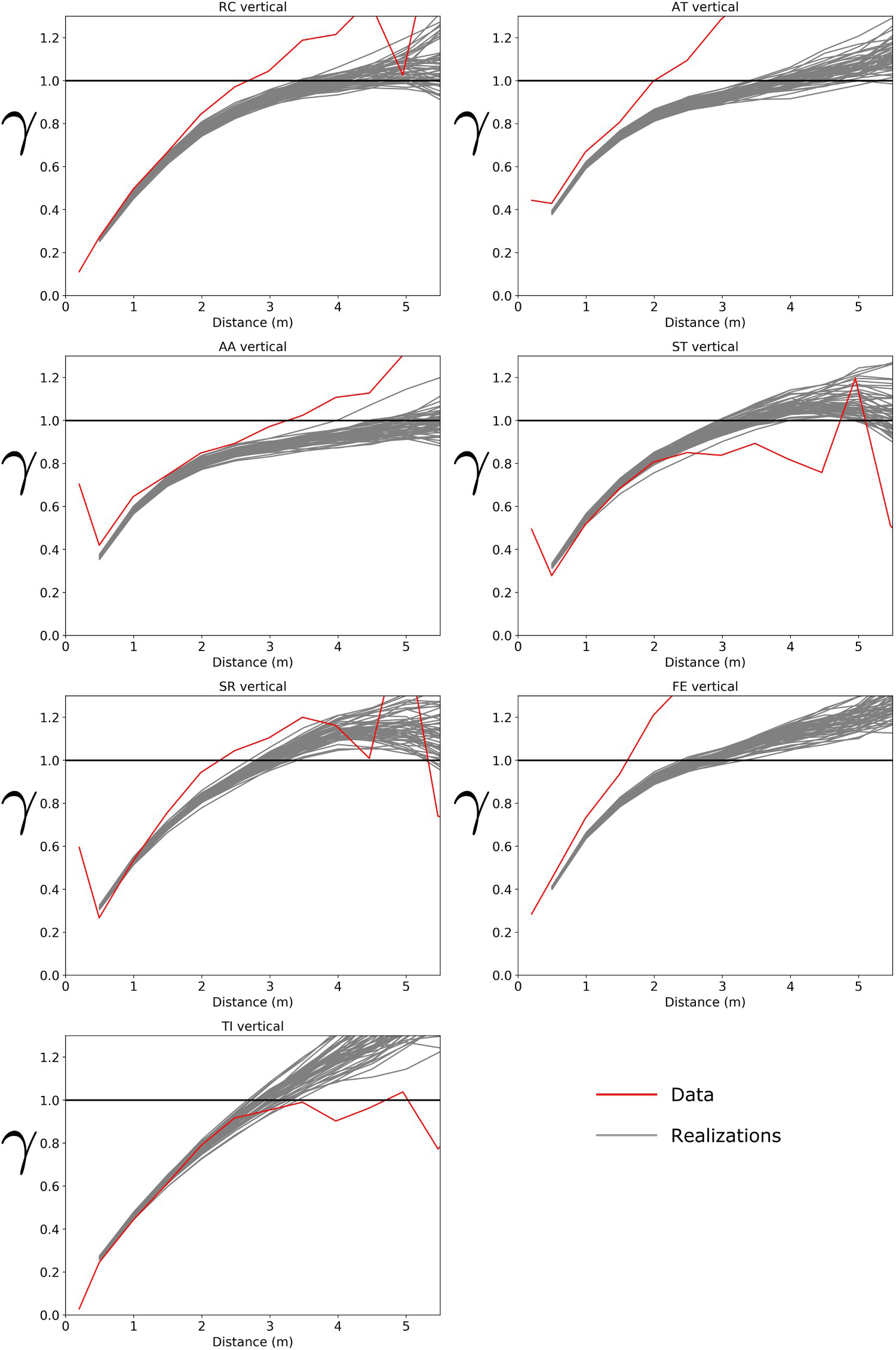
In general, the variable RC had better variogram reproduction than the others (Figures 7 and 8). This result probably occurred because RC was transformed only once (PPMT) before the simulation. On the other hand, the remaining variables were transformed twice (ratios and PPMT). Applying only PPMT directly to all the original variables may improve the variogram reproduction. However, the resulting simulations are likely to violate the sum and fraction constraints.
Reproduction of bivariate relationships
The coefficients of correlation of the data and of the first realisation were compared (Figure 9). The coefficients of correlation of the realisation are similar to those of the data, as the points are close to the line y = x (Figure 9).
Scatter plot between the coefficients of correlation of the data and of the first realisation.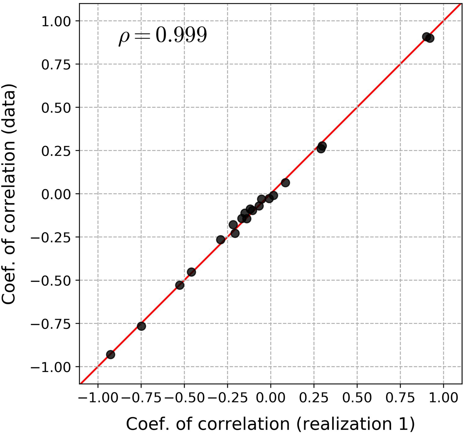
The scatter plots between AT and RC and AT and FE of the data and of the first realisation were compared (Figure 10(a–d)). The scatter plots were coloured by the probability density, which was obtained with kernel density estimation. The scatter plots of the first realisation are similar to the scatter plots of the data. These results support the work of Barnett et al. (2016), which showed good reproduction of bivariate relationships for geostatistical simulations done with PPMT.
Scatter plot between AT and RC of the data (a) and the first realisation (b) and scatter plot between AT and FE of the data (c) and the first realisation (d).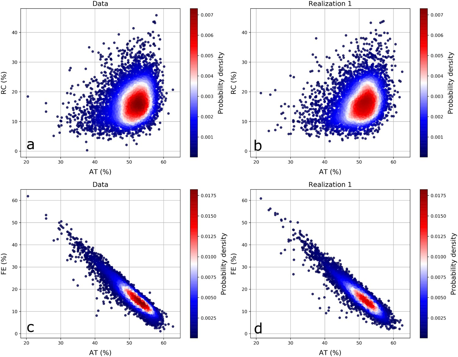
Check of sum constraint
The histogram of the sum of AT, ST, FE and TI of the first realisation is shown in Figure 11. The simulations honoured the sum constraint, as the maximum of the sum is below 100 (see Figure 11). These results agree with those presented by Barnett and Deutsch (2012). Barnett and Deutsch (2012) used additive log-ratios to consider the sum constraint. The additive log-ratios are similar to the ratios A used in this paper.
Histogram of the sum of AT, ST, FE and TI of the first realisation.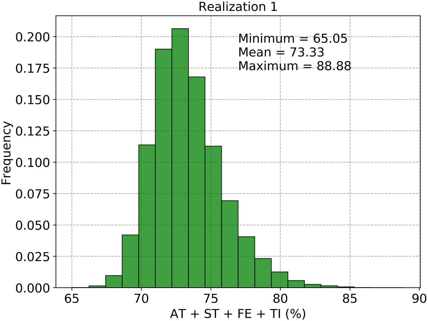
Check of fraction constraint
The scatter plots between the total and fractional grades of the first realisation are shown in Figure 12. The simulations respected the fraction constraints, as AT is greater than AA (Figure 12(a)) and ST is greater than SR (Figure 12(b)). The workflow applied the normal score transform (first step of PPMT) to the fraction ratios. The maximum of the fraction ratios is below one. As the normal score back-transformation avoids extrapolation, the simulated values of the fraction ratios were below one. As a result, the multiplication of the simulated total grades by the simulated fraction ratios resulted in simulated fractional grades that honoured the fraction constraints.
Scatter plot between AT and AA (a) and ST and SR (b) of the first realisation.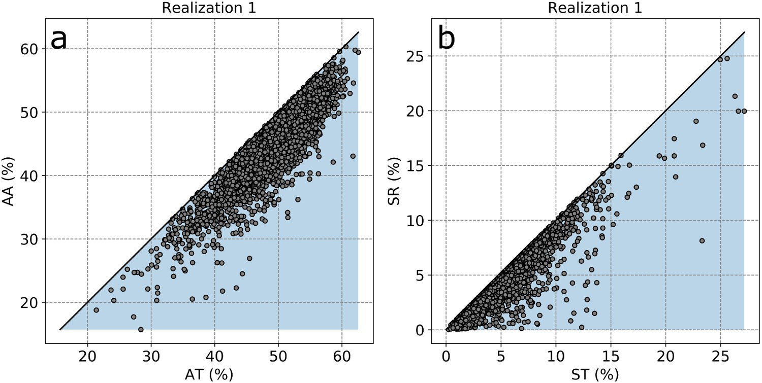
Conclusions
The paper presented a workflow to address the problem of multivariate geostatistical simulations with sum and fraction constraints. Sum constraints mean that the sum of some variables may not exceed or must equal a critical value. Fraction constraints mean that one variable may not exceed other variable and occur when one variable is a fraction of other, such as fractional and total grades. The methodology was illustrated in a case study with data derived from a bauxite deposit in Brazil.
First, variables with constraints were re-expressed as ratios. For the variables with sum constraint, the ratio consisted of obtaining a filler variable and dividing the original variables by the filler variable. For the variables with fraction constraint, we used fraction ratios, which are the ratio between the fractional and total grade. Second, the ratios were transformed using PPMT (PPMT). The transformed variables were simulated independently using SGS and back-transformed. The inverses of the ratios were applied to obtain the simulations of the original variables.
The realisations showed satisfactory reproduction of the variograms, histograms and bivariate relationships. Furthermore, the realisations honoured the sum and fraction constraints. The use of ratios was effective to consider sum and fraction constraints. Moreover, the use of PPMT preserved the relationships between the variables. Although the use of ratios and the PPMT have been established in the literature, this paper presents a novel case study combining transformation techniques and demonstrates that sum and ratio constraints can be enforced in a practical workflow.
Footnotes
Disclosure statement
No potential conflict of interest was reported by the authors.