
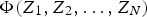
Abstract
Geostatistics aims to spatially model multiple correlated attributes with some under-sampled variables. Missing samples can distort the data set statistics, and for the model to be consistent, it is necessary to understand the mechanisms that cause the missing data (MD). There are three mechanisms that can govern MD: Missing Completely at Random (MCAR), Missing at Random (MAR) and Missing Not At Random (MNAR). More specifically, when there is a systematic difference between measured and the missing samples, the data is subject to the MNAR mechanism, which leads to biases in the final model if not dealt with adequately. A case is presented where an under-sampled attribute, U (ppm), is modelled to infer its values over the study area through co-simulation approach and an univariate simulation performed on an artificially complete set, considering the MNAR mechanism, which shows a
 reduction in the relative estimation errors compared to the co-simulated model.
Introduction
The evaluation of mineral resources is linked to geostatistical methods which describe spatially continuous phenomena using samples collected over an area of interest. Considering
 a random vector of multiple correlated attributes, generally one is interested in predicting the spatial variability, global and local means, probability of being under or over a threshold, and so on (Chilès and Delfiner 1999; Diggle et al. 2010) of this set of variables, so as to determine the viability of the mining endeavour. The need to characterise the region, allied with the economic aspects of data exploration, lead to preferential and unequal sampling, which can distort the known distribution of the variables (Diggle et al. 2010; Enders 2010; da Silva and Costa 2016), which in turn results in biased models of the features of the phenomenon.
Therefore, heterotopic configurations must be taken into account. The classical geostatiscal approaches for dealing with multivariate heterotopic data sets are based on cokriging (Marechal 1970) systems and the use of the linear model of corregionalisation (LMC). Cokriging, however, can have some practical complexities with the growing number of variables considered in the analysis. Moreover, not only can its use be extremely tedious, it does not account for different reasons for the under-sampling of some attributes in relation to others.
In the field of statistics, under-sampled variables are referred to as missing data (MD) variables, and there has been extensive research dedicated to understanding the implications of absent information (Rubin 1976; Little and Rubin 2002; Schafer and Graham 2002). According to Rubin (1976), it is possible to relate missing and measured values through three distinct mechanisms: missing completely at random (MCAR), missing at random (MAR), and missing not at random (MNAR).
Considering a random vector of N variables,
 , the MCAR mechanism occurs when the probability of missing a value of
 does not depend on the values of
 nor on any of the
 variables observed. The MAR mechanism occurs when the probability of missing values of
 depends on one or more of the
 variables observed, but not on
 itself. Finally, the MNAR mechanism occurs when the probability of missing a value of
 depends on
 itself and on some of the
 variables. For example, in mining, one of the variables of interest often has a very low-grade zone within the deposit, and it is not beneficial to sample such a zone.
MD theory (Rubin 1976) has demonstrated that accounting for the correct MD mechanism leads to an estimation of the statistical parameters that are more representative of the sampled population. Methods such as complete case analysis applied to MD cases are only adequate if the mechanism in action is MCAR; while bias is generated in the final estimations when the other two mechanisms occur. MCAR, however, does not govern most practical cases. Consequently, identification of the missing conditions is crucial for the final model to be adequately built and be coherent with the reality at hand.
For the MAR case, the state of the art approaches are maximum likelihood estimation (MLE) and multiple imputation (MI) (Rubin 1988; Schafer and Graham 2002; Enders 2010). The first assumes that the data follow a Gaussian distribution and aims at estimating the distribution parameters that best fit the data; the second is based on Bayesian statistics, creating multiple complete scenarios that are analysed and combined to obtain one final complete set. In the geological framework, imputation can be compelling for multivariate data sets that do not have the same number of samples when the modelling aims to obtain information for all variables simultaneously. Ren (2007) proposed a method based on the work of Doyen et al. (1996) that stands on the Bayesian MI framework, aiming to build a posterior distribution by considering the spatial relations that exist between the variables, from which the MD can be sampled and imputed for the set. This approach, called Bayesian updating (BU), has proved to be adequate when the missing mechanism is MAR (Ren 2007; Barnett and Deutsch 2008, 2012).
The MNAR mechanism is far more complex to deal with: the MD carry important information about the data population that cannot be ignored. Doing so may bias the generated estimates. Models that acknowledge the MNAR mechanism alleviate the bias by incorporating a description of the probability of the MD (Enders 2010). However, such a description is extremely challenging since there is no access to the MD. According to Rubin (1987), when the data are missing under the MNAR mechanism, there is a systematic difference between the observed and the MD. As there is no direct way to estimate the bias generated by the sampling discrepancy, the model is sensitive to the different hypotheses adopted.
Therefore, Rubin (1987) proposed that distinct models should be generated under several hypotheses, using the empirical knowledge about the problem at hand. Thus, the models must be easily interchangeable, that is, produce different outcomes originating from alterations in the model assumptions. Even if more complex approaches may generate more accurate results, simple modifications such as those described tend to be applied, due to their feasibility.
It has been suggested to apply fixed transforms to the values imputed when assuming the MAR mechanism ad hoc, transforming the estimates to imputed values under the MNAR mechanism (Rubin 1987; Enders 2010). For instance, if multiple scenarios are generated through MI, all the values imputed in each scenario could undergo a transformation to compensate for the difference between the data originally observed and the samples not collected. If there is sampling of two statistically distinct ore zones, and one of the attributes is under-sampled, and there is a reason to believe that the missing samples correspond to a low-grade zone, all values imputed through MI, BU or MLE will over-estimate the ore grade. So, to compensate, after the imputation process has taken place, the imputed values should be reduced. Rubin (1987) suggested that this compensation should be
 , although this value is arbitrary. Along the same lines, Cohen (1988) proposed that the transform should be proportional to one-half of the standard deviation from an imputed scenario, having a direct impact on the mean of the data set (Enders 2010). The present paper presents the use of the maximum relative deviation obtained by a process similar to holdout cross-validation, to compensate for an over- or under-estimation of the values imputed through BU (da Silva and Costa 2016).
Materials and methods
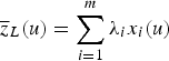
As mentioned before, in the geostatistical framework, it is important to incorporate all the information available, and their statistical relations. Doyen et al. (1996) proposed a simplified collocated cokriging approach, in which the estimates were obtained directly by updating, through Baye's rule, the kriged (Matheron 1963) estimated variance with the secondary collocated sample, without the need to refer to the cross-covariance and the cokriging system (Marechal 1970). In that paper, only the knowledge of the correlation coefficients between the primary and secondary variables was required. Later, Doyen's approach was adapted to the MD problem, where the same idea is employed by aiming to obtain solely the missing samples before any simulation or estimation model is built. The Bayesian approach uses three different distributions: prior, likelihood, and posterior. In this framework, it is assumed that the data are Gaussian distributed, so their distribution is completely described by their mean and variance. For the prior distribution, information coming from the incomplete variable, referred to as primary, is used to build the prior distribution. The information coming from a set of other variables, referred to as secondary, is used to build the likelihood distribution. Finally, the product of the first two generates the posterior distribution from which the missing samples will be drawn.
Bayesian updating - BU
Assume that the random variable Z is the primary variable and assume that it is stationary over the area A. Assume that
 is a set of secondary variables and that Z and
 are multi-Gaussian. The primary mean,
 , and variance
 , at the location u where the sampling is missing, are respectively, obtained from Equations (1) and (2):
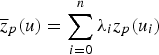
 s are the simple kriging weights,
 is the location of the ith sample and
 is the covariance between the estimated point
 and the sample
 . The weights are obtained from Equation (3):
 is the covariance between the primary data,
 and
and
 and
and
 is the covariance between the estimated point
 and the primary data
 . These are the results of the simple kriging of the primary variable. The likelihood distribution is defined by the mean,
 , and variance,
 , obtained from Equations (4) and (5):
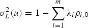
 is the secondary information on location u, and the weights
 s are calculated using the correlation between the primary and secondary variables according to Equation (6):
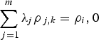
 is the correlation between the two secondary variables, while
 is the correlation between the primary and secondary variables. Once the prior and likelihood distribution are defined, the posterior distribution is determined by their product:
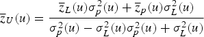
 is the mean and
 is the variance of the posterior distribution. Since this distribution is Gaussian and completely determined by these two parameters, the imputed values may be drawn from it by Monte Carlo simulation (Ren 2007; Barnett and Deutsch 2008, 2012) generating as many complete scenarios as desired.
After imputing the missing samples of the data set, one can apply the fixed transforms to compensate for the systematic difference between the observed and MD (Rubin 1987). The fixed transform presented in this paper is that the values imputed be corrected proportionally to the maximum error obtained through a holdout cross-validation performed on the imputed values through BU. The fixed transform herein proposed is described by Equations (9) and (10):
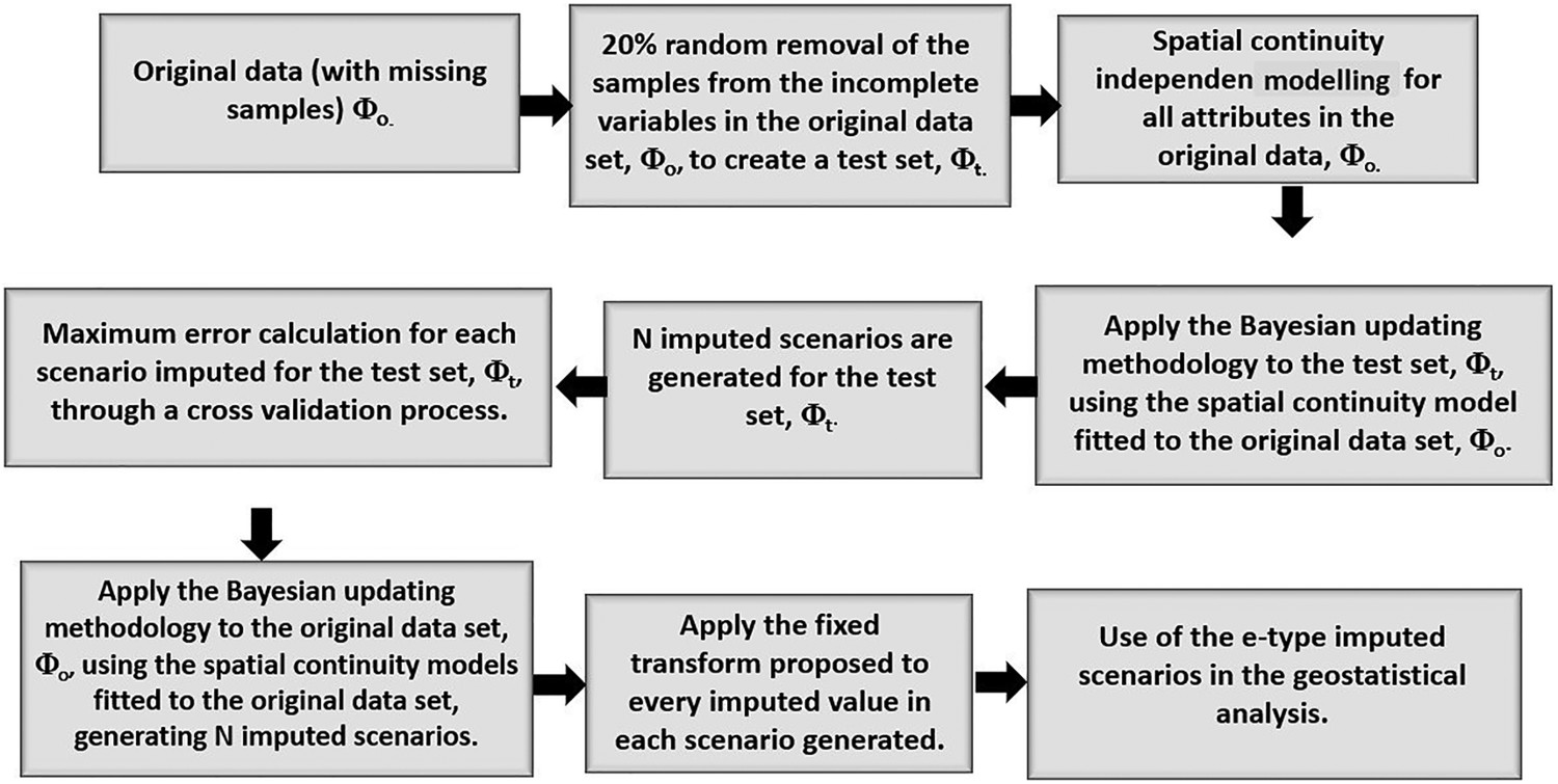
Work flow proposed to the case study.

 is the error obtained through cross-validation on the BU's jth scenario at the ith location,
 is the imputed value at the ith location with a missing sample, and
 is the measured sample at the ith location.
 is the maximum value of
 obtained in the jth scenario; and
 is the updated value after the fixed transform has been applied to the jth BU scenario. The cross-validation is performed on a test set composed by
 of the samples of the primary variable, randomly drawn. The work flow applied to the case study is described in Figure 1.
Data set
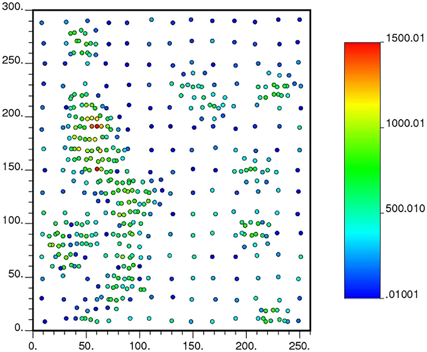
The case study was performed on the Walker Lake data set (Isaaks and Srivastava, 1989b), which contains 470 sampled locations. The data were collected in three stages. In the first stage, 195 locations were sampled, spaced approximately every 20 m. At this stage, information was collected from the two variables: V (ppm), which is continuous, and T, which is categorical. In the second stage, the sampling spacing was reduced to 10 m, and after that, in the last stage, to 5 m, aiming to characterise high-grade zones. In the two last stages, the variable U (ppm) was also collected. Therefore, the 195 samples missing from the U variable are of low grade, tending to be an MNAR mechanism. In the case study presented, the two continuous variables will be used, V as an auxiliary variable to help in estimating U, and the exhaustive data of Walker Lake data set is used as the benchmark for evaluating the quality of the model. Figures 2 and 3 show the location maps for the samples of the primary variable U and the auxiliary variable V (Isaaks and Srivastava, 1989b).
Location map for the U (ppm) variable with 275 samples. Location map for the V variable with 470 samples.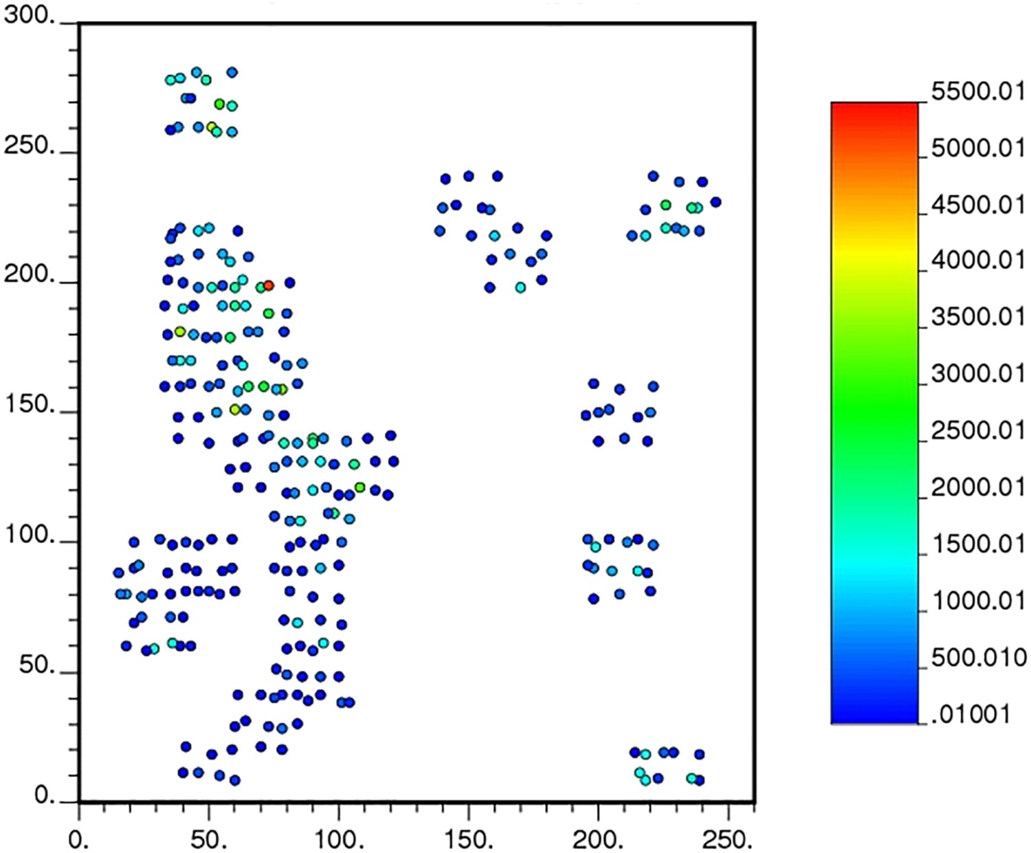
Walker Lake sample set and exhaustive data set statistics.
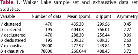
Note that the declustered statistics for V approximate their counterparts for the exhaustive data set: the mean value for the sample set with 470 samples of V, is 288.30 and its counterpart, the exhaustive mean, is 277.97, which is a
 relative deviation. For U, the declustered statistics differ greatly from the exhaustive data statistics. The mean of U over the 275 samples is 509.32, but for the exhaustive data it is 266.044, with a relative deviation of
 . This is also observed for the other statistics presented in Table 1. Therefore, it is seen that the sampling process of U is not representative, which suggests that the MD is not MAR.
The aim of this study is to perform a geostatistical modelling of U, which is under-sampled in the data set, taking into account that ignoring the MD can affect negatively the final model. Then, the approach herein presented will be applied to the problem. Taking advantage of the fact that the two variables at hand have a correlation of
 , the imputation will be performed by first applying Bayesian updating to a test set, computing the maximum error for all scenarios created at this stage, then Bayesian updating will be applied to the original sample set, and afterwards all the imputed values will be transformed using Equation (10). Consequently, the outcome will compensate for the MNAR mechanism. For the purposes of comparison, a transform similar to Equation 10 will be applied to the imputed data set using the constant of
 of the imputed values suggested by Rubin (1987), and the imputed set without any transformation applied will be retained to compare the performance of the models. A sequential Gaussian co-simulation (Verly 1993) was also run on the data to evaluate whether the method proposed in this paper will lead to a model as good as that obtained by the classical geostatistical approach. In the end, all four models generated will be compared to the exhaustive data, for validation.
Both Bayesian updating (Ren 2007; Barnett and Deutsch 2008, 2012) and sequential Gaussian simulation (Isaaks 1990) are based on the assumption of multivariate normal distributions due to mathematical tractability. Geologic data, however, in most cases do not conform to the normal distribution behaviour. The convention is, therefore, to transform each variable in the data set to a Gaussian distribution prior to imputation and simulation. To perform such a transform, there are numerous methods, such as normal score transform (nscore) (Deutsch and Journel 1992), Projection Pursuit Multivariate transform (PPMT) (Barnett et al. 2014) and Stepwise Conditional transform (SCT) (Rosenblatt 1952). The last two need isotopic sampling, which is the very aim of this paper, consequently, the nscore transform was applied to the data. A univariate Gaussian distribution is fully characterised by its mean m and standard deviation
 . The probability density function is given by:
Normally distributed variables do not show proportional effect, that is, no relation between mean and variance should be observed. The bi-normality of the transformed variables, prior to the imputation and simulation steps, are verified through moving window statistics. The scatter plot of the mean m and variance
Scatter plot for the mean (m) and variance (
Scatter plot for the mean, (m), and variance, (
 is shown for the nscore transform of the U variable (Figure 4) and the nscore transform of the V variable (Figure 5) and it can be seen that no proportional effect is detected for the transformed variables. According to Goovaerts (1997), if the bi-normality assumption is valid, then the multi-normality is assumed for the model.
 ), of the U variable moving window statistics.
 ), of the V variable moving window statistics.


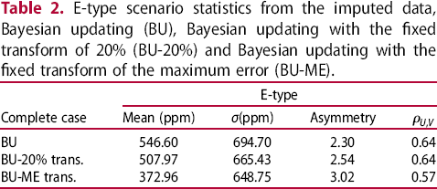
 of the samples of U. It is important to highlight that the removal at this stage to separate a test set needs to be random, so that no additional bias is inserted in the imputations as well as additional distortions to the sample set statistics. The maximum error computation results from the imputations for the removed samples and the comparison to their measured value. At this point, there are three complete cases created through Bayesian updating, each with 50 scenarios. Table 2 shows the statistics obtained for the average complete scenario (E-type) obtained through Bayesian updating, in each of three models generated: maximum error fixed transform (BU-ME),
 fixed transform (BU-
 ), and the Bayesian updating model where no fixed transform was applied (BU).
E-type scenario statistics from the imputed data, Bayesian updating (BU), Bayesian updating with the fixed transform of (BU-20%) and Bayesian updating with the fixed transform of the maximum error (BU-ME).

Barnett and Deutsch (2008) recommend that for each simulation realisation a different imputed scenario be used as input data, propagating the uncertainty of the imputed values into the final model. As the input data for the co-simulation approach is unique (only the original data set is normally informed with no uncertainty associated with it), the E-type imputed cases were used in the SGS approach in order to obtain a description for the U variable over the entire study area. Subsequently, a sequential Gaussian co-simulation (Verly 1993) was performed on U, to evaluate whether the approach herein presented is equally adequate to the problem, resulting in four models: SGS with maximum error E-type imputed, referred to as SGS-ME; the SGS with the transform of
 , referred to as SGS-20; the SGS with the imputed data through Bayesian updating without any fixed transform applied, referred to as SGS-BU, and a co-simulated model, referred to as COSGS. Lastly, all four models were compared to the exhaustive statistics to evaluate their performance.
Each E-type imputed data was declustered using the moving window method and normalised using


To perform co-simulation, the variables considered need not be equally sampled; therefore, a linear model of corregionalisation is used to model the direct and cross-covariances simultaneously. In this case, the fitting began with the V variable, which has more samples in the data set, and is therefore easier to set the spatial continuity. The models fitted to V and U are shown in Equations (19)–(21).


Knowing the exhaustive data set, with 78, 000 samples of V and U, allows evaluating the quality of the models generated through each of the approaches mentioned in this paper. It is expected that the models reproduce the data statistics. Figure 6–9 compare the histograms of the simulated models to that of the exhaustive U data set.
Cumulative histograms of the SGS-BU simulated model (solid lines) and cumulative histogram of the exhaustive Walker Lake data set (dashed line). Cumulative histograms of the SGS-20 simulated model (solid lines) and cumulative histogram of the exhaustive Walker Lake data set (dashed line). Cumulative histograms of the COSGS simulated model (solid lines) and cumulative histogram of the exhaustive Walker Lake data set (dashed line). Cumulative histograms of the SGS-ME simulated model (solid lines) and cumulative histogram of the exhaustive Walker Lake data set (dashed line).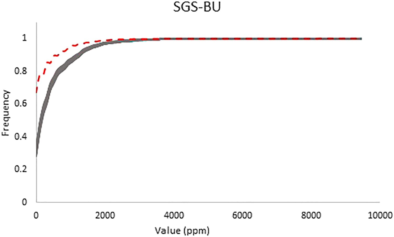
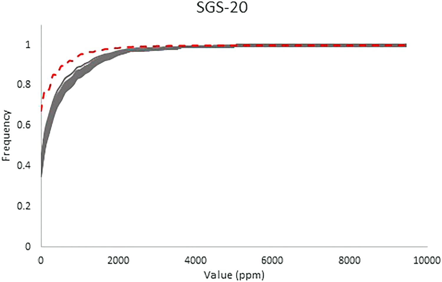
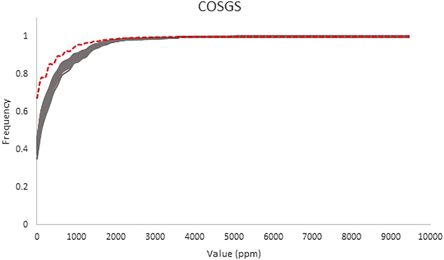
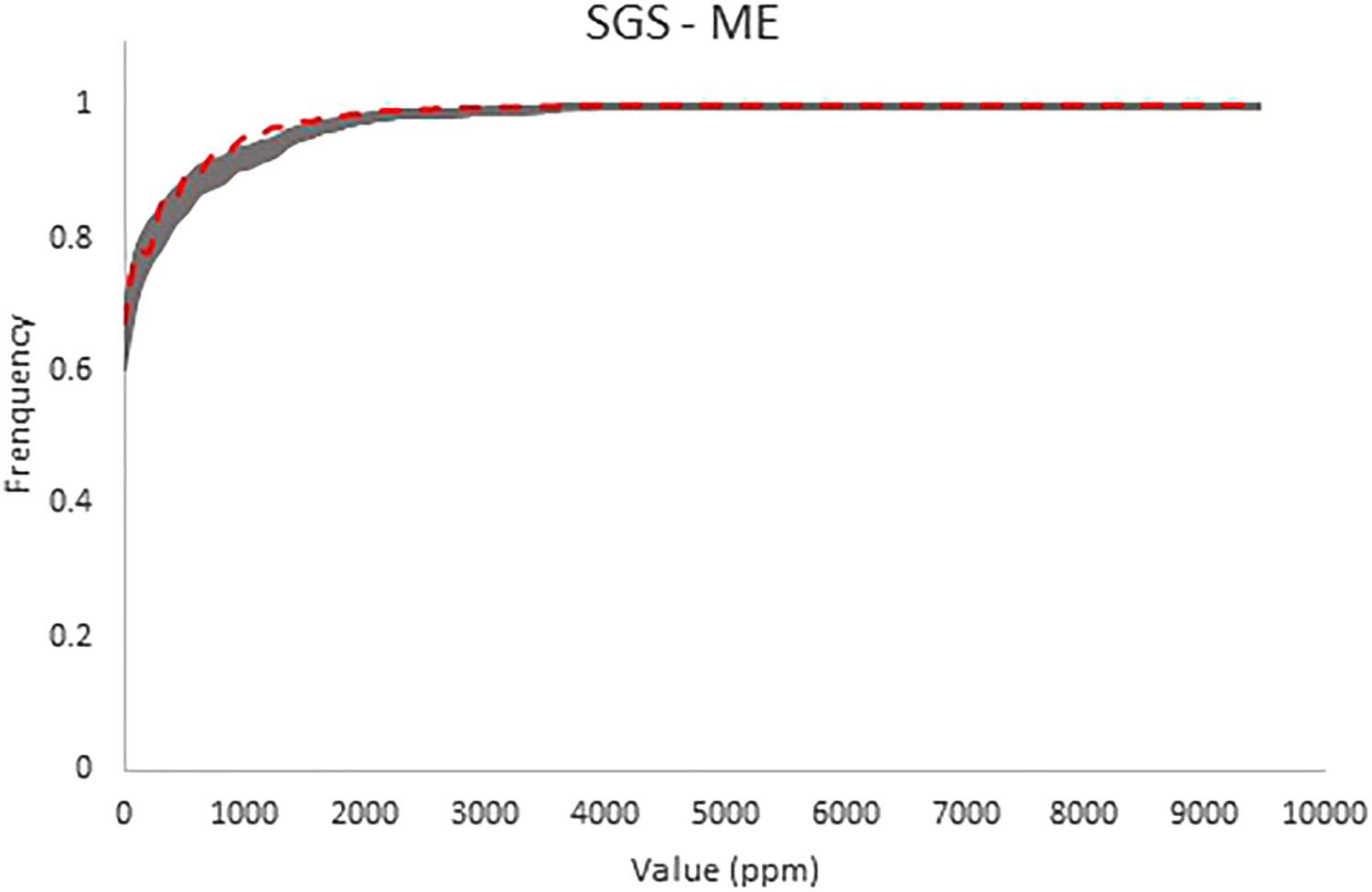
 constant applied to the imputed values, underestimate the frequency of low values in the distributions as well as the co-simulated model, Figure 8. But the simulation performed using the E-type imputed scenario where the maximum error fixed transform was applied (SGS-ME) to the imputed values is the only model that did not underestimate the frequency of the low values of U Figure 9, presenting a behaviour similar to that of the exhaustive data set. This behaviour is corroborated by the statistics shown in Table 3.
Comparison of the ranges of values obtained for some statistics in the 50 simulated models from each method and reference set, Walker Lake exhaustive.
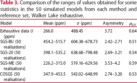

From Table 3, it can be seen that the simulated SGS-BU, SGS-20 and the COSGS present a systematic bias relative to the exhaustive data set mean, overestimating its value. The skewness is underestimated by all three models mentioned, also consisting in a systematic bias in relation to this parameter. For the SGS-ME model, the exhaustive mean is embedded in the range of mean values obtained by the 50 realisations generated, as is the skewness. None of the models generated were able to reproduce the variance of the exhaustive data, even though it is lower than the variance of the incomplete data, it is not low enough when compared to the variability of the whole population. According to Diggle et al. (2010), due to the preferential sampling, the empirical variance function is highly affected by the sampling design, since it is conditioned to the locations where the information is collected, hence its inability to reproduce the exhaustive variance.
Additionally, the correlation obtained from the simulated scenarios is more similar to the incomplete data correlation with V (ppm) than the exhaustive data correlation, the value obtained with the SGS-ME model being the closest to the correlation presented by the exhaustive data set, with a deviation of
 . In the case of the co-simulated model, the relative deviation is
 . In the SGS-ME simulation, if one is interested in the global mean estimate, the average deviation is
 of the exhaustive value. For the co-simulated model, the global mean estimate has an average relative deviation of
 , overestimating the exhaustive data mean, and, in the best case scenario, it has a relative deviation of approximately
 .
.
The behaviour of the local mean throughout the deposit was also evaluated. The area was divided into 13 m bands from West to East, and 15 m bands from North to South. The means of the exhaustive data and the simulated models were calculated within these bands. Figures 10 through 13 summarise the behaviour of the local mean.
Swath plots for the SGS-BU simulated model (solid lines) and the exhaustive data set (dashed line).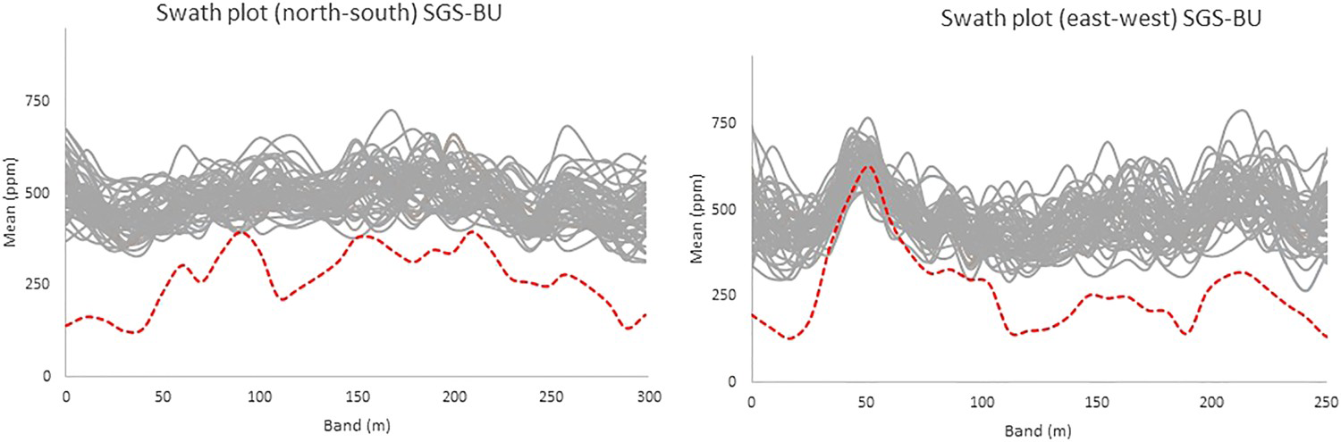
Note the SGS-BU overestimates the mean values in all locations within the area (Figure 10). The sampling favoured high values and under-sampled the distribution at its lower tail. This has affected the quality of the model in such a way that, even if the missing values were imputed, the resulting model would still be biased if the MNAR mechanism is not taken into account.
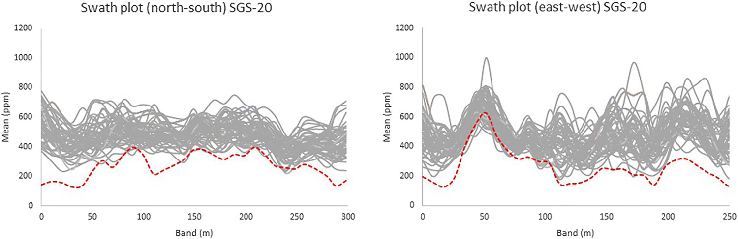
The SGS-20 simulated model takes the MNAR mechanism into consideration, through Rubin (1987) suggested fixed transform, using a compensation of
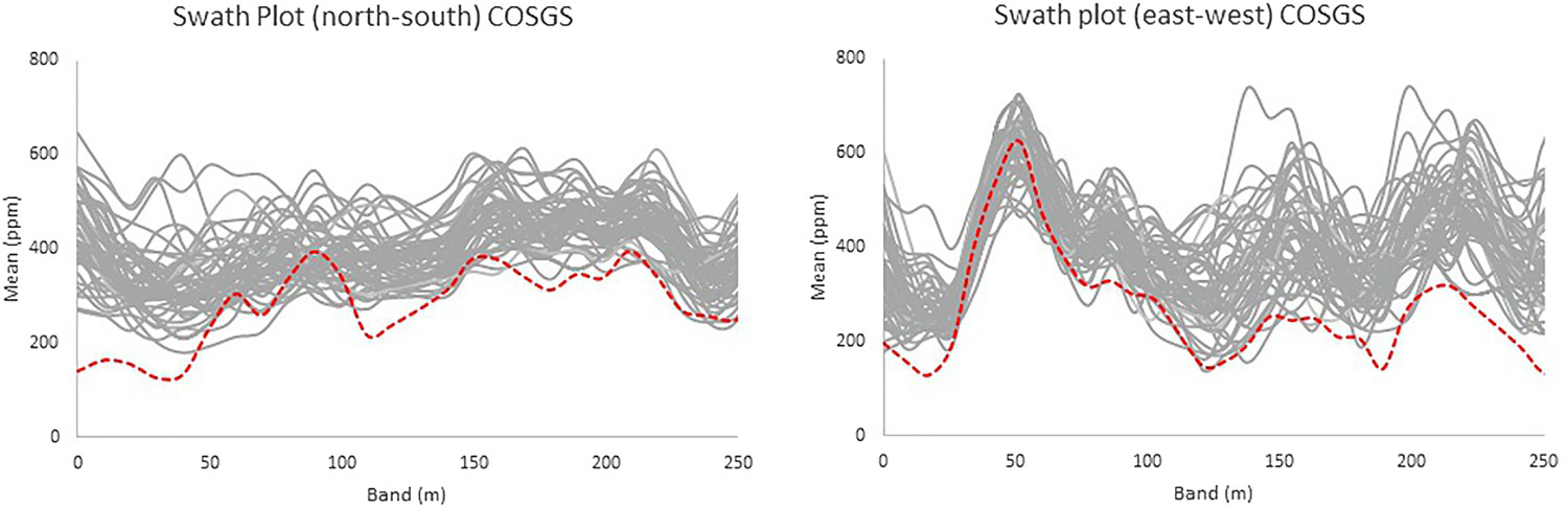
Swath plots for the SGS-20 simulated model (solid lines) and the exhaustive data set (dashed line). Swath plots for the COSGS simulated model (solid lines) and the exhaustive data set (dashed line). to lower every imputed value and consequently populate the lower tail of the distribution. Under the circumstances of attribute U being highly variable, and in the presence of outliers, such a fixed transform is not enough to compensate for the extremely misrepresented distribution (Figure 11). Also, the swath plots obtained for the COSGS and SGS-ME models are shown. Note that the COSGS model also has a bias relative to the exhaustive data local mean values (Figure 12), even though it is not as significant as those of SGS-BU and SGS-20. If the sampling of one of the attributes has MD, and it could have resulted from an MNAR mechanism, the other explanatory attributes from the set may not be able to correct the distribution of the under-sampled variable.
For the SGS-ME, the mean is well reproduced throughout the area (Figure 13), as this distribution parameter is corrected by the fixed transform applied. The more variable the attribute is, and in the presence of preferential sampling, the more disperse will be the error distribution from the imputed values be (Diggle et al. 2010). As for this case, it was adequate to transform the imputed values proportionally to the imputation error. It enabled populating the lower tail of the distribution, even though the variability of the population was not correctly reproduced, it being somewhere in between the under-sampled data statistics and the exhaustive data set statistics. Lastly, the uncertainty space is evaluated using accuracy plots (Pyrcz and Deutsch 2002). Figures 14–17 show the accuracy plot for each model generated.
Swath plots for the SGS-ME simulated model (solid lines) and the exhaustive data set (dashed line). Accuracy plot for U (ppm) SGS-BU simulated model. Accuracy plot for U (ppm) SGS-20 simulated model. Accuracy plot for U (ppm) COSGS simulated model. Accuracy plot for U (ppm) SGS-ME simulated model.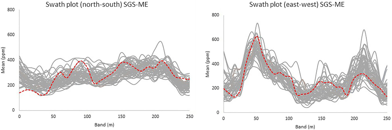
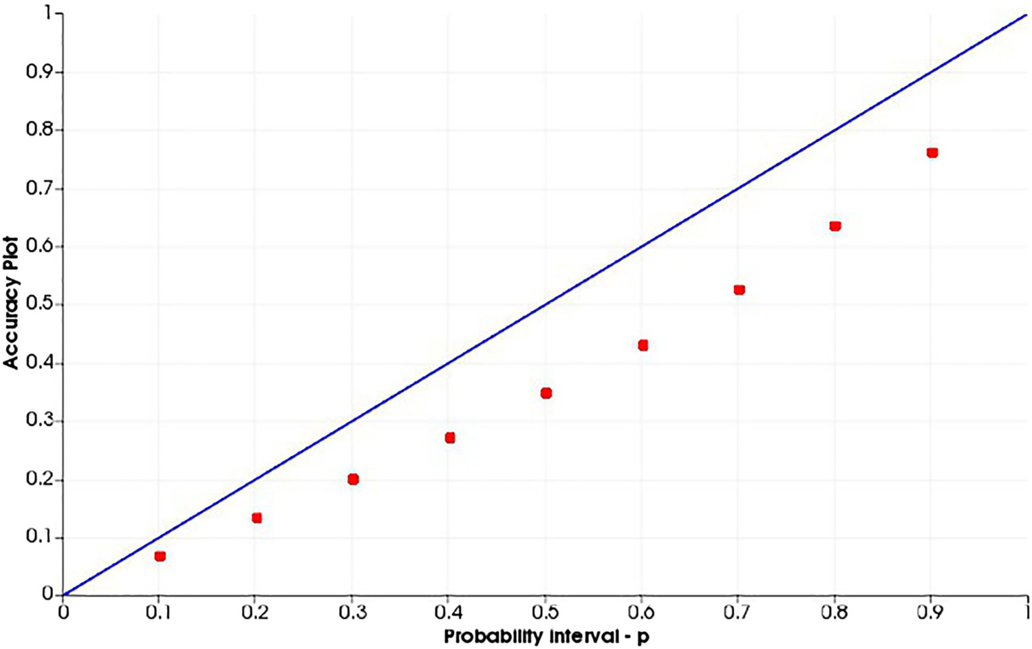
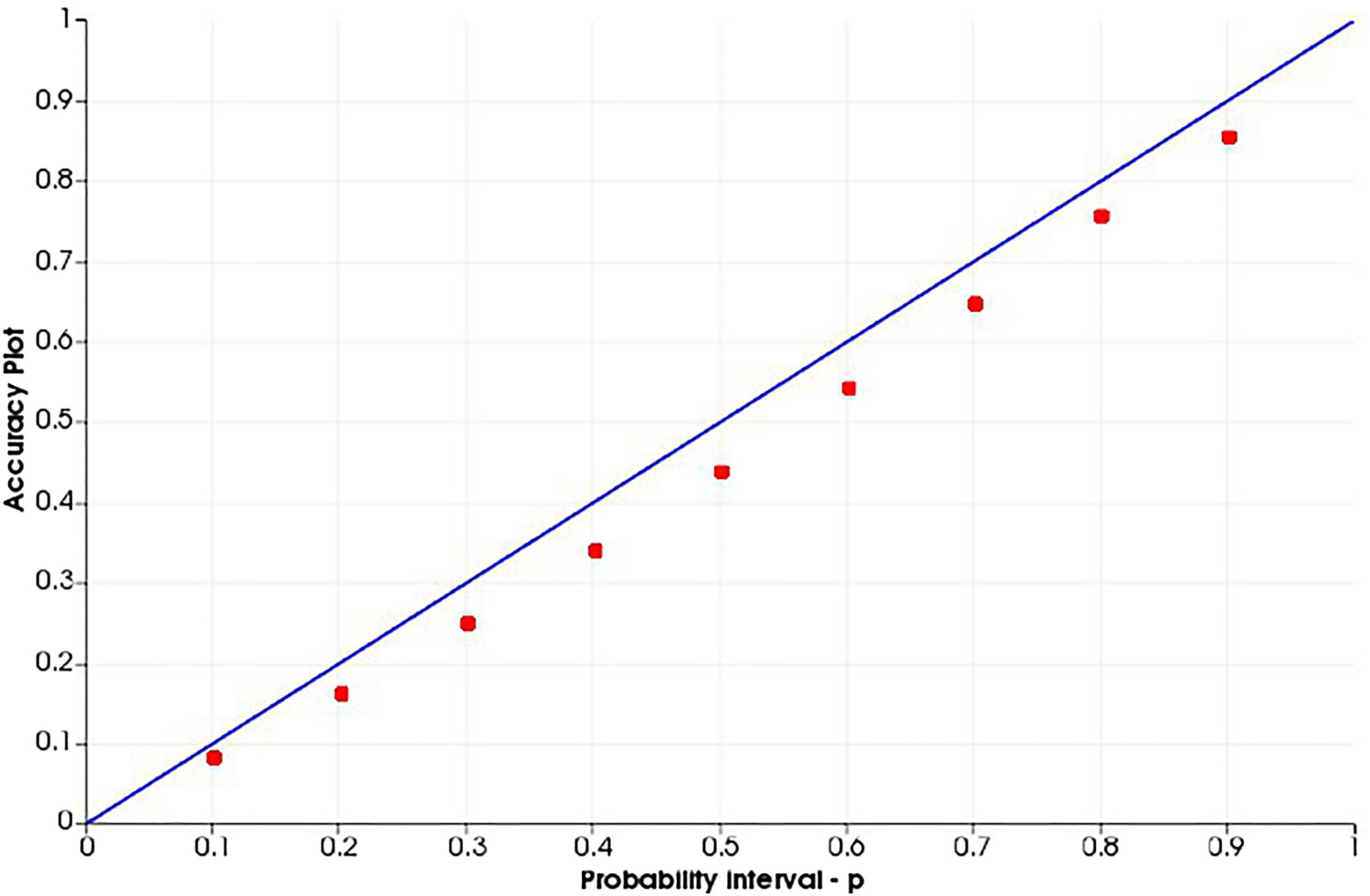
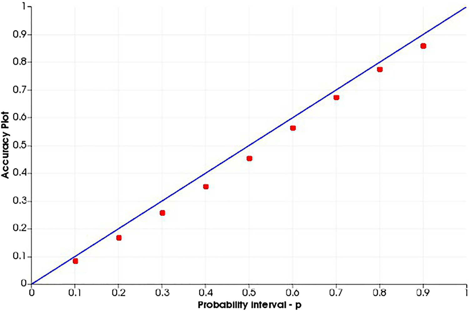
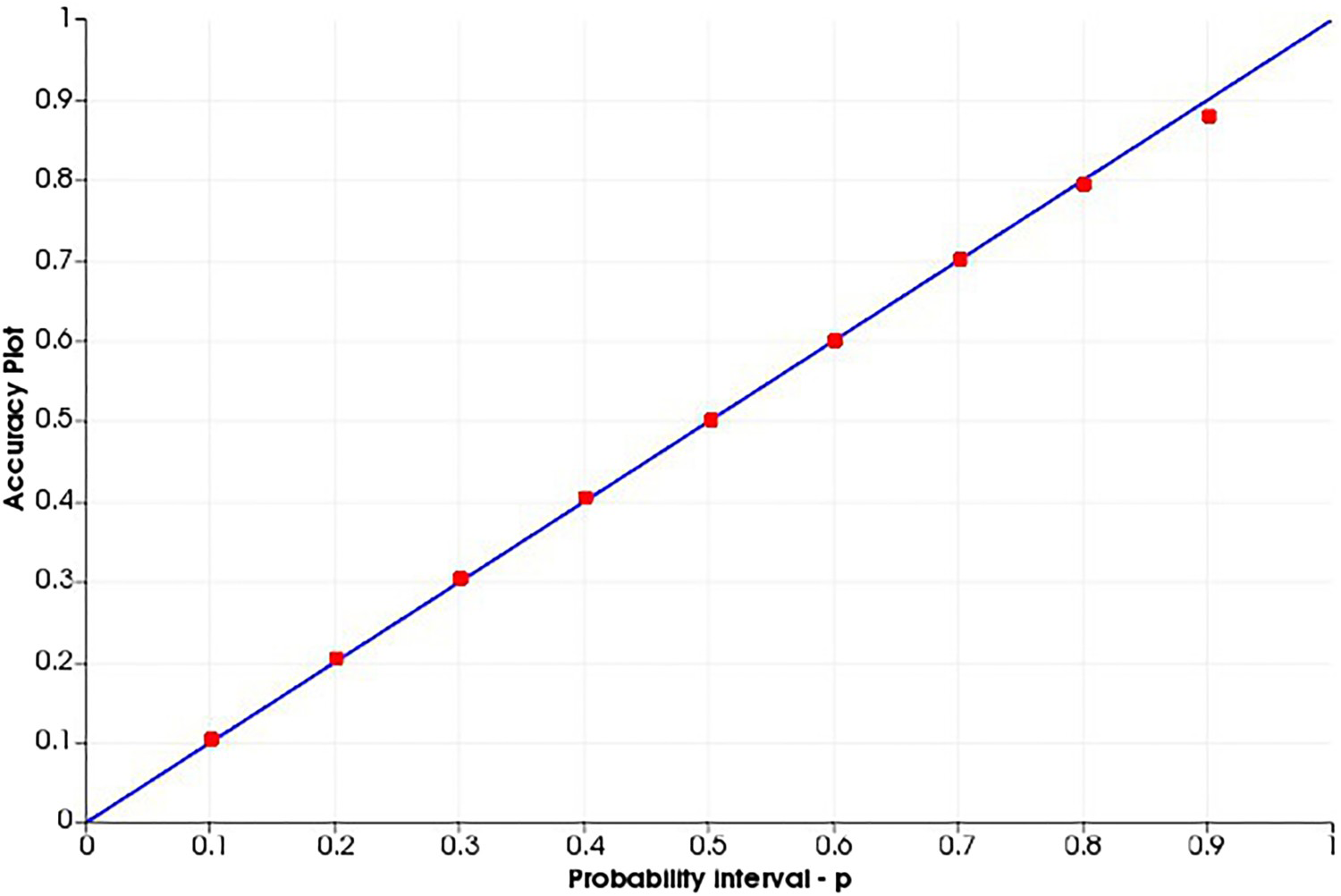
Analysing the accuracy plots, it is important that the plot of the dots be along the
 line, since this would mean that the simulated space is accurate and precise. This is performed as a cross-validation, using the true values to compare with the simulated values. At each probability interval, the true value should occur proportionally within the range of values simulated. The models generated from the SGS-BU (Figure 14) and SGS-20 (Figure 15) are imprecise and inaccurate, having lower occurrences of the true values in the range of simulated values for all probability intervals. For the COSGS model (Figure 16), even though less inaccurate, the probabilities are lower than expected at every probability interval. For the SGS-ME model (Figure 17), the realisations are precise and accurate.
The results of this case study lead to the belief that in facing a situation of MD, data imputation does not suffice if the missing mechanism is not taken into account. Bayesian updating has proved to be adequate in many other geological cases, where the MD were the result of a mechanism. Nevertheless, if there is reason to believe that the data were sampled at some preferential region or grade value zone, the MNAR mechanism should be considered, or the user may produce a biased model. Also, the fixed transform has great value and should be further explored, due to its practical applicability and easy communicability between generated models. In this case study, the high variability from the under-sampled attribute showed that a fixed transform based on the imputation error is more adequate than the use of an arbitrary constant, which should be considered only in situations where the analyst has great knowledge about the sampling process. The co-simulation, in this particular case, was not able to correct the bias that originated from the (under) sampling procedure. Lastly, the final model obtained through SGS-ME leads to an adequate result without the need of using the classical approach of co-simulation, being easier to apply, as it is implemented in a univariate SGS work flow.
Footnotes
Acknowledgments
The authors would like to thank the Brazilian National Research Agency (CNPq) for supporting the Mineral Exploration and Mining Planning Research Unit (LPM) at the Universidade Federal do Rio Grande do Sul.
Disclosure statement
No potential conflict of interest was reported by the authors.