Boundary simulation – a hierarchical approach for multiple categories

Abstract

Geological modelling is a crucial step in mineral resource evaluation. The traditional approach to modelling the volumetric limits, explicit modelling, presents a series of limitations and disadvantages which makes it costly to assess the uncertainty in relation to the location of the limits between different domains in the mineral deposit. In many cases, the geological model can be a source of crucial uncertainty, for this reason, the uncertainty associated with the geological model must be assessed. This paper proposes a method for assessing geological model uncertainty by simulating the contacts between different domains in a mineral deposit in a hierarchical manner using signed distances. The proposed method was demonstrated in a case study conducted on a porphyry copper deposit. Models generated by the proposed method do not show much noise, as this method leads to continuous contacts between domains while the volume variation and contacts characteristics can be controlled by the parameters. Results are compared to sequential indicator simulation, a traditionally used technique to model geobodies and assess its uncertainty.

Keywords

Geologic model boundary simulation implicit modelling signed distances uncertainty assess

1 Introduction

Geological modelling is a crucial step in mineral resource evaluation. Geostatistical estimates and simulations require stationary random functions within predetermined volumetric limits.

The traditional approach to modelling the volumetric limits, which represents each mineral domain in the mineral deposit, is through a 3D triangulation of polygons or strings representing the solid body. The polygonal/string outlines or polylines are drawn by a geomodeller on a series of offset cross sections using expert judgment. The cross sections are then joined by tie-lines in order to guide the connectivity between poly-line sections during the 3D triangulation of the solid boundary. This procedure is referred to as an explicit model of the solid since the bounding surface is defined unequivocally by the 3D coordinates positioning the patchwork of triangles (McLennan and Deutsch 2006).

Although the traditional methodology is straightforward and simple, the main reasons for its wide implementation in practice, and that modern mining software provides computational tools to visualise the drilling data and streamline the digitisation process (Silva 2015), there is a series of limitations and disadvantages. The process is tedious and time-consuming, manually digitising the polylines and joining them by tie-lines, requires a lot of time from an experienced professional. In highly complex deposits, it is not uncommon for the geomodeller to work for up to 3 months on the explicit geological model. The geometry of geological bodies often needs to be simplified so that the model is conceived in a timely manner. For this reason, for most mines, only one model is built and maintained, there is rarely an opportunity to model alternative geological interpretations and compare resource estimates or simulations based on different models (Cowan et al. 2003).

Models created explicitly are subjective and not replicable. The modelled volumes are essentially composed of a series of small subjective decisions, since each point of the polyline in each section is chosen by a geomodeller. Inevitably, the ‘signature’ of the professional is printed within the limits of the geological domains. Different geomodellers create different models from the same dataset. Furthermore, explicit models are inflexible, it is laborious and time-consuming to update explicit models as new data is obtained since a new manual digitisation is required.

Due to the onerosity in building multiple explicit geological models, it is costly to assess the uncertainty in relation to the location of the limits between the different domains in the mineral deposit. In addition to the tedious manual re-digitising of polylines and re-triangulation, there is no direct way to incorporate multiple realisation for locations of limits between different domains.

In many cases, the geological model can be a source of crucial uncertainty. In gold vein deposits, for example, mineralised volume is a vital economic indicator for project management. Ignoring volumetric uncertainty, considering only a single explicit geological model, can be devastating for the enterprise. The uncertainty associated with the geological model must be assessed.

The need to assess the uncertainty associated with the geological model drove the development of automatic stochastic methods for geological modelling. This paper proposes a method for assessing geologic model uncertainty by simulating the contacts between the different domains based on Wilde and Deutsch (2012) method. The method relies only on composited drill holes X, Y and Z coordinates and the rock type property. Since Wilde and Deutsch (2012) method works only for binary cases and naively making its application in multiple domain cases is time-consuming, overlapping or producing blocks not assigned by any category. We proposed an algorithm to automatically group different lithologies and a workflow for simulating each group individually and then reconstruct the multicategorical geological model from it in a hierarchical manner. The method is straightforward, and the results are replicable, incorporating incremental geological data is easy and fast, and the generated models are realistic.

2 Background

There are several methodologies available for modelling categorical variables and their uncertainty assess. These methods can be divided into object-based and cell-based approaches.

The object-based frameworks (Pyrcz and Deutsch 2014) are focused on the reproduction of morphological shapes such as meandering channels in fluvial environments. Usually, the models are not conditioned to the data (Silva 2018). Object-based methods have no application in mining so far, finding application in the oil industry.

Cell-based methods, in contrast, are conditioned to the data and widely used in the mining industry. One of the cell-based alternatives to generate multiple geological model realisations is multipoint simulation (MPS) that uses a training image to create conditional probabilities. Each realisation aims to reproduce geological characteristics of the training images. The method was initially proposed by Guardiano and Srivastava (1993), but several variations were developed based on the initial method (Boucher 2009; Strebelle 2002).

Sequential indicator simulation (Alabert 1987) is a widely used cell-based technique for categorical variable models. The algorithm is robust and provides a straightforward way to transfer uncertainty in categories through the resulting numerical models. However, the models can appear very patchy and unstructured (Deutsch 2006).

There is also the family of truncated Gaussian methods. These methods are applied when lithologies occur in a fixed order, such as stratigraphic sequences. The basic idea behind truncated Gaussian simulations (Matheron et al. 1987) is to start out by simulating one Gaussian variable at every cell in the study area and then use a truncation rule to convert these values back into categorical values. In many cases, the truncated Gaussian approach proves to be too restrictive, so it can be extended to two or more Gaussian variables. This adaptation is called truncated pluri-Gaussian (Armstrong et al. 2011). The concept of using a truncation rule in more than one dimension is limiting as the geological interpretation degrades when higher number of categories and/or Gaussian variables are considered. For this reason, a new adaptation was developed: hierarchical truncated pluri-Gaussian (Silva and Deutsch 2019) utilises a tree structure to define the truncation rules in one dimension. This facilitates the definition of the mapping between continuous and categorical space making it possible to efficiently utilise any number of Gaussian variables for the modelling of a categorical variable.

Another family of cell-based methods is the implicit modelling. Implicit models are created from scattered sample data, usually categorical and structural. An implicit function or implicit model provides a continuous mathematical representation of the attribute throughout the volume (a scalar field). Implicit models contain an infinite number of isosurfaces, and to visualise a geological model an isosurface must be extracted from the model, usually the zero isosurface. Different volume functions can be used in geological modelling.

Potential fields (Chilès et al. 2004; Calcagno et al. 2008; Lajaunie et al. 1997) derive the implicit model by universal cokriging of surface intersection and structural orientation data. It is straightforward to visualise the uncertainty in the boundary surface placement. However, the procedure is not simple, the covariance of the potential field is particularly difficult to infer, since there are no hard potential field data available (McLennan and Deutsch 2006). Gonçalves et al. (2017) gave a machine learning approach to the method. de la Varga et al. (2019) developed an open-source stochastic geological modelling tool that assess uncertainty using potential fields and a Bayesian approach.

Other authors built implicit models and assessed geological model uncertainty using structural data. Lindsay et al. (2012) examined the uncertainty introduced by geological orientation data by producing a suite of implicit 3d models generated from orientation measurements subjected to uncertainty simulations. Pakyuz-Charrier et al. (2018) studied the effect of structural input data uncertainty propagation in implicit 3D geological modelling. Caumon et al. (2007) assessed geological model uncertainty by perturbing the geological parameters such as fault and horizon surfaces.

An implicit model can also be derived from signed distance functions (Cowan et al. 2002, 2003) which have gained considerable popularity due to its simplicity and efficiency. Lillah and Boisvert (2013) modified the signed distances approach to incorporate non-stationarities in the form of a locally varying anisotropy field used in kriging and sequential Gaussian simulation allowing for a stochastic assessment of uncertainty. Silva (2015) used signed distances to create data driven training images for MPS combining deterministic and stochastic geologic interpretations to transfer the essential geological features into geostatistical models. Yang et al. (2019) proposed a method that directly assesses and visualises the uncertainty of geological surfaces, using signed distances, by the means of stochastic motion. Wilde and Deutsch (2012) proposed a method that consists in determining a parameter C that controls the geological unit uncertainty, simulating uniform values within an uncertainty zone, and then comparing the simulated values with the interpolated values, thus creating equiprobable realisations for a geologic unit. The method produces geologically realistic realisations. However, it works only for binary cases.

3 Methodology

In order to illustrate the proposed methodology the Swiss Jura dataset (Goovaerts 1997) is used. The data set comprises 259 samples and a rock-type (RT) property. A map with the location of the samples is shown in Figure 1.

Figure 1

Location map of the 259 samples of the Swiss Jura dataset.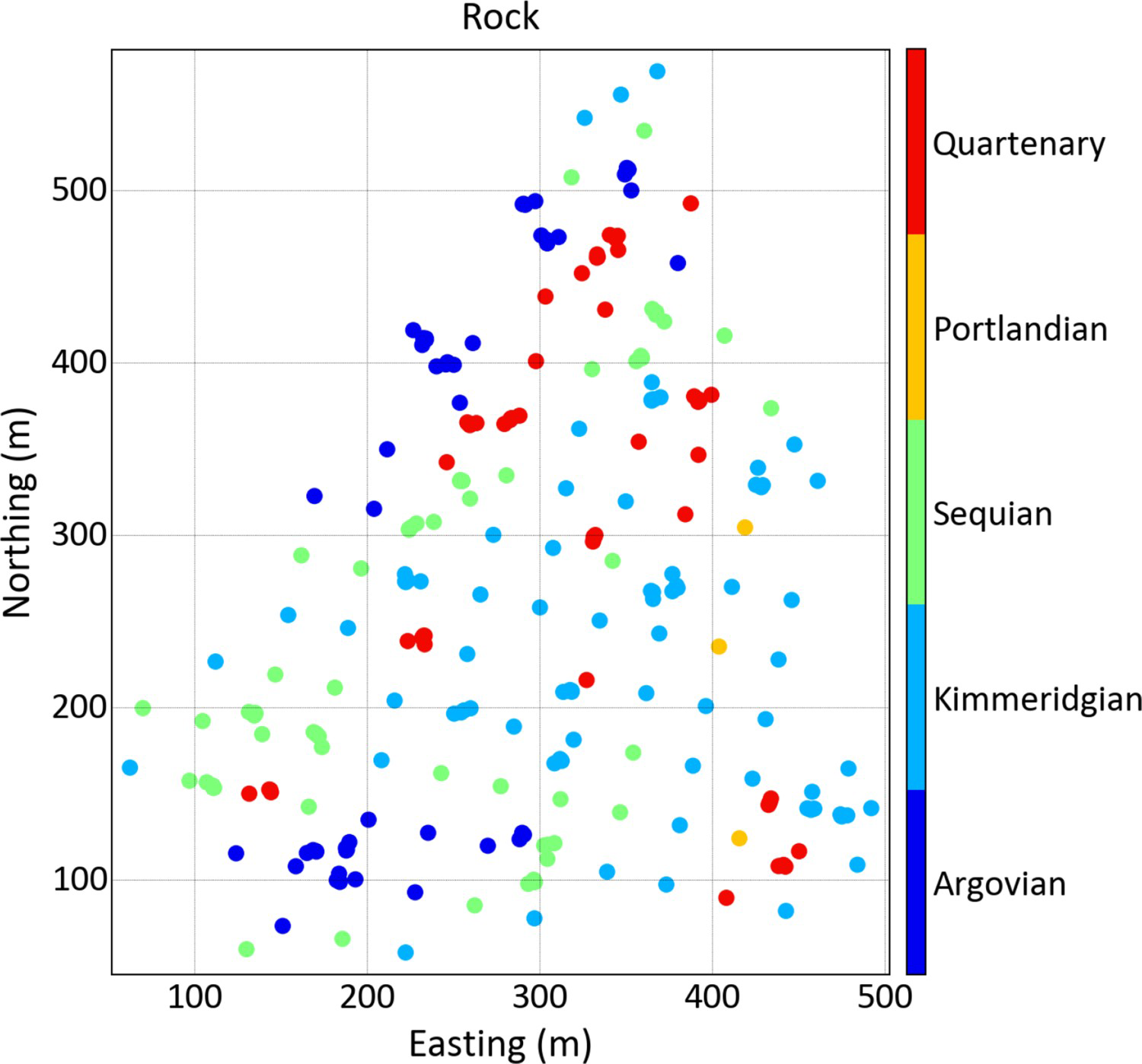

The RT variable has five categories: Argovian; Kimmeridgian; Sequian; Portlandian and Quaternary. The area is covered partially with evenly spaced samples with some areas that are densely sampled with additional clusters of data.

3.1 Grouping

The first step of the workflow is to defining groups of samples which represents the contacts between different lithologies of the mineral deposit. The grouping can be explicitly defined by a geomodeller or can be automatically done by the proposed algorithm.

The marching cubes algorithm (Lorensen and Cline 1987) is applied to a proto geological model to identify and count the contacts. The proto model can be created by nearest neighbour, support vector machine, indicator kriging or signed distances on a coarser grid than the final simulation grid to speed up the process. In this algorithm, a cube composed by eight cells in three dimensions or four cells in two dimensions runs through the proto model grid, as shown in Figure 2, from left to right and from top to bottom visiting all grid nodes. The algorithm checks whether at least one of the nodes that make up the cube belongs to a different category than the others. In that case, those blocks are marked as a contact and this contact is counted.

Figure 2

Schematic drawing showing the functioning of the marching cubes algorithm: the cube runs through the entire grid identifying and counting the contacts.

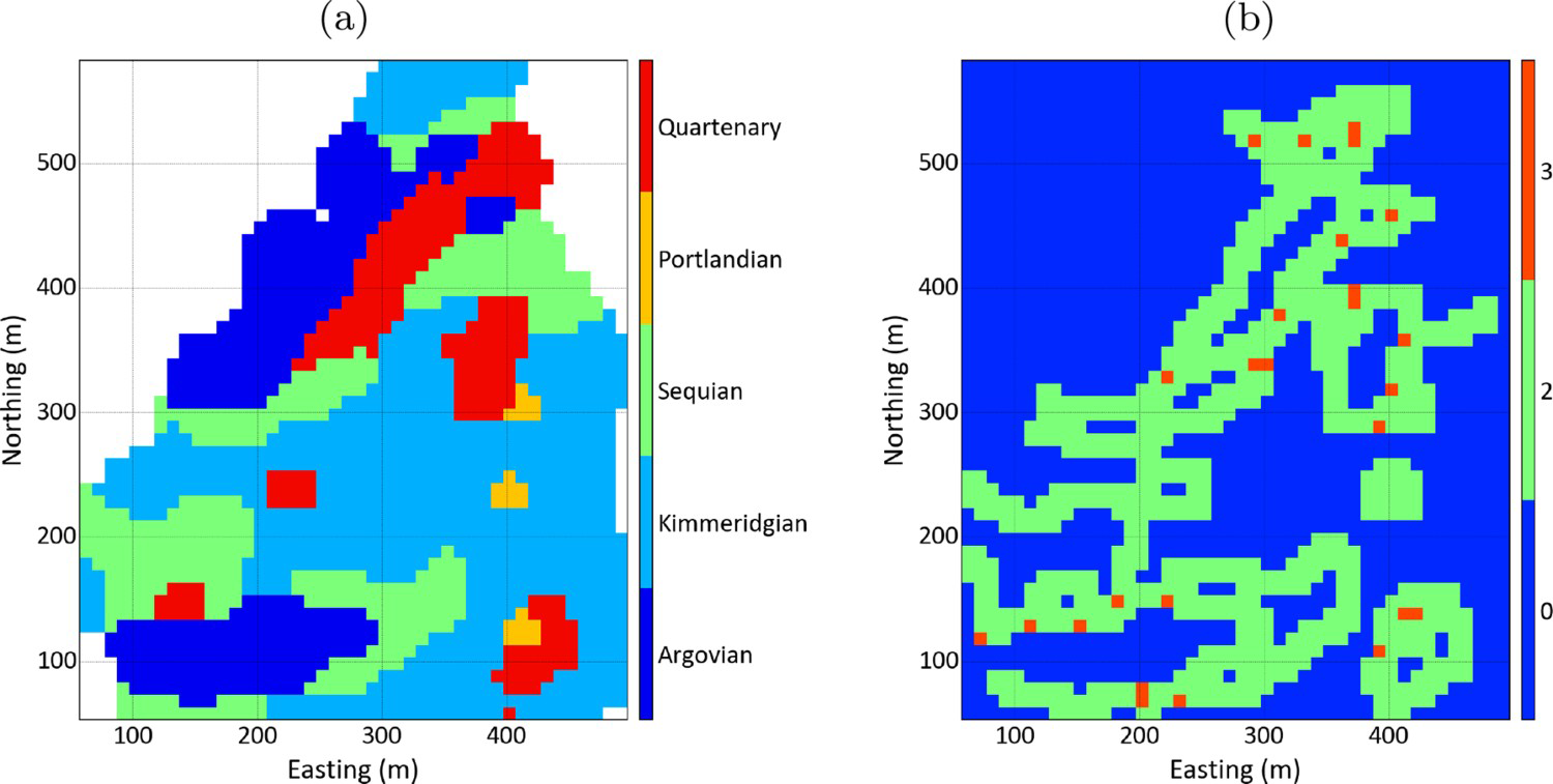
Figure 3 show a proto geological model created from the Swiss Jura dataset using signed distances on a m grid. The grid resolution can change the final grouping.

Figure 3

Proto model and blocks marked as contacts for the Swiss Jura: (a) proto geological model and (b) blocks marked as contacts. Colours indicate how many categories are part of that contact.

The number of contacts between categories, counted by the marching cubes algorithm, is presented in Table 1.

Table 1

Contacts count by the Marching cubes algorithm.

Kimmeridgian; Sequian	134
Argovian; Sequian	74
Kimmeridgian; Quartenary	66
Argovian; Quartenary	45
Sequian; Quartenary	40
Kimmeridgian; Portlandian	23
Portlandian; Quartenary	9
Argovian; Kimmeridgian	8
Argovian; Kimmeridgian; Sequian	7
Argovian; Sequian; Quartenary	6
Kimmeridgian; Portlandian; Quartenary	4
Kimmeridgian; Sequian; Quartenary	4

To define the (K−1) groups, where K is the number of categories in the dataset, Algorithm 1 is applied. The first groups represent the most frequent contacts. In the initial iteration, the variable i is the even number 0, and the algorithm will create a group where Kimmeridgian and Sequian samples are coded as 1 and other category samples are coded as 0. In the second iteration, the variable i receives the odd number 1, therefore the algorithm will create a group where Kimmeridgian samples are coded as 1 and Sequian are coded as 0. Besides that, the algorithm will remove from contacts count table any contacts in which Kimmeridgian or Sequian is part, namely, lines 1, 2, 3, 5, 6 and 7. The variable i presents the even value of 2 in the third iteration, thus a group is created where Argovian and Quartenary samples are coded as 1 and other categories from the contacts count table, after removing lines samples, are coded as 0, as this is the most frequent contact after removing the lines. The algorithm assumes that the first (K−1) most frequent contacts will be between two, not more, categories, which is reasonable in a geological context.

Algorithm 1: Defining the groups from contacts count table

for i in (K-1) do

if i%2!=0 then

1. Creates a group: categories of the most frequent contact are coded as 1, other categories are coded as 0

else

1. Creates a group: one category of the most frequent contact is coded as 1, the other is coded as 0

2. Removes from the contacts count list all contacts that contain at least one of the most frequent contact categories

end

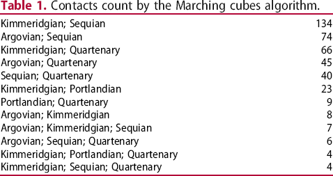
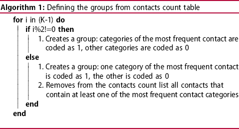
Figure 4 shows the hierarchy rule defined by the proposed algorithm to the Swiss Jura proto model.

Figure 4

Hierarchy rule defined by the proposed algorithm.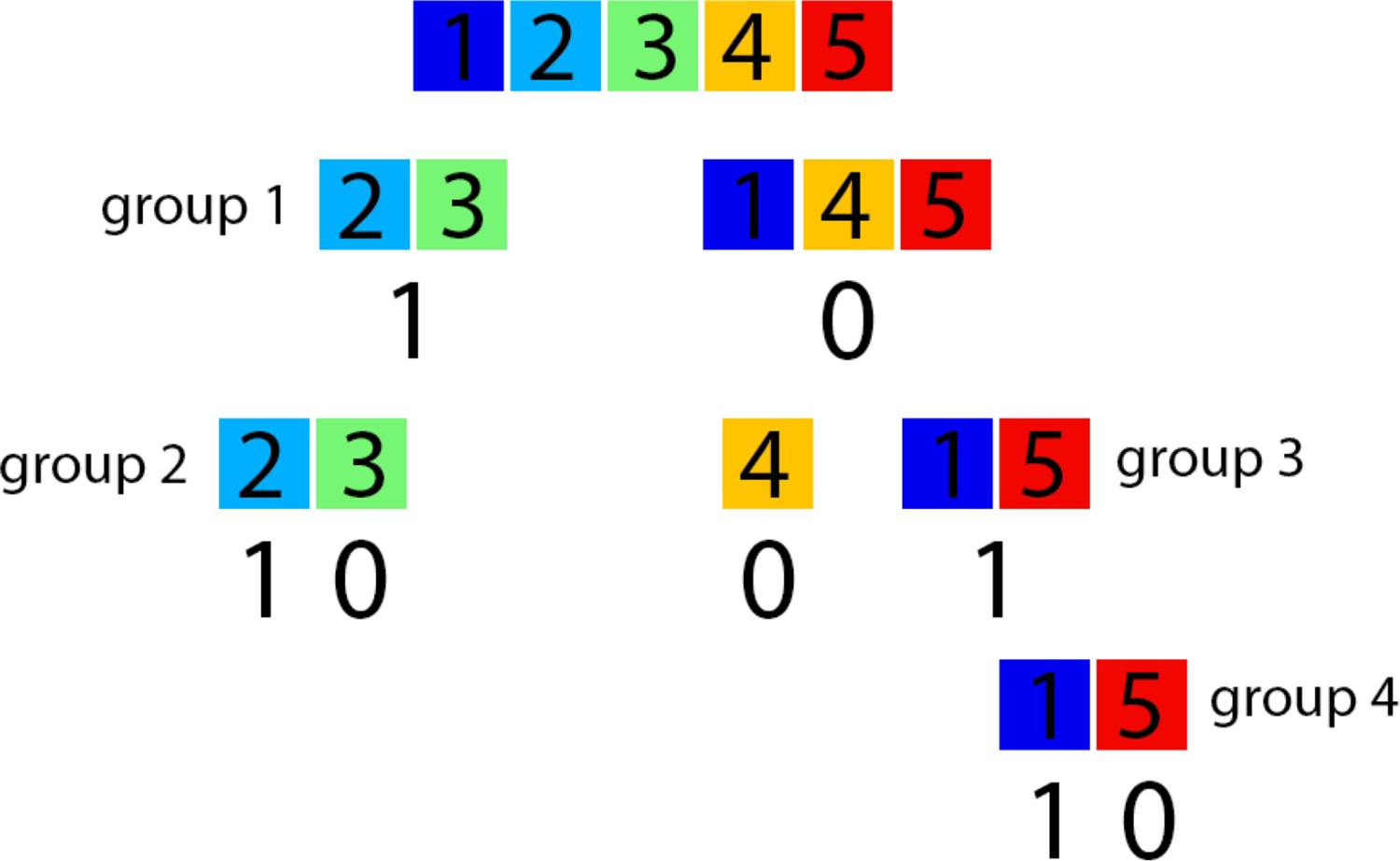

The four groups of sample data generated with the hierarchy rule are presented in Figure 5. The first group contains all samples from the dataset while the others are subsets.

Figure 5

Location maps of the samples for the four groups: (a) Group 1, (b) Group 2, (c) Group 3, (d) Group 4.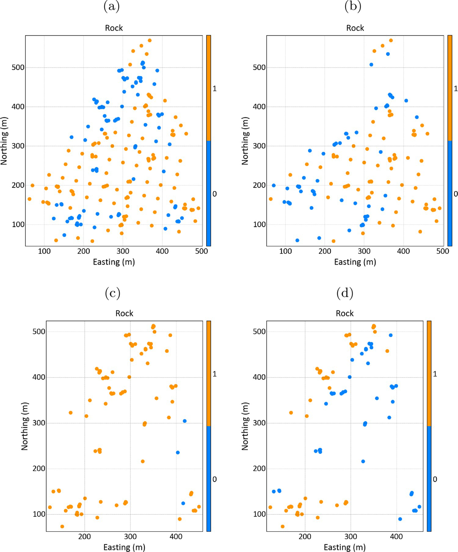

3.2 Uncertainty parameter C

It is necessary to define an uncertainty zone around the contacts between indicators in each group. Blocks located outside the zone are considered as belonging to a particular indicator, while blocks within the zone will have their uncertainty assessed. The uncertainty zone is obtained using a parameter C to create and control the zone thickness/size.

The choice of parameter C depends on the level of accuracy required against the time taken to calibrate the parameter. Thus the parameter can be determined in different ways: the empirical determination is based on predetermined values and knowledge about the phenomenon considering the sampling geometry and the experience of the geomodeller (Karpekov and Deutsch 2016). Partial calibration compares interpolated models with a base reference model. The C value is determined from the interpretation of representative sections and expert judgment, and it is expected that the calibrated uncertainty interval is reasonable. Conversely, the total calibration is time-consuming and laborious, and it uses numerous reference models to determine the parameter C (Karpekov and Deutsch 2016). For each reference model, an optimisation algorithm is used to calculate the parameter C, and for a single iteration it is necessary to interpolate all the reference models with the same parameter C. In order to achieve full calibration, multiple iterations are required using different values for the parameter C, which demands a large computational effort and increases the size and number of reference models used (Munroe and Deutsch 2008).

The calibration can also be performed by a method similar to jackknife cross validation methodology (Wilde and Deutsch 2012), using only the data to calibrate the parameter C with low computational demand and high automatisation.

The first step in the calibration of C by jackknife is to remove a subset of the data. This can be done by randomly choosing drillholes to exclude. A proper calibration study involves generating several jackknife sets with different proportions (50% to 10%) of data removed and different configurations of data removed (Manchuck and Deutsch 2015). Distance function values are then calculated for the remaining data with an initial value of C=0. These distance function data are used to condition the estimate of distance function at each of the jackknife data locations. There are four possible outcomes resulting from this estimation. The location could be: correctly estimated to be outside the domain, correctly estimated to be inside the domain, incorrectly estimated to be outside the domain and incorrectly estimated to be inside the domain. The main interest is in the number of data that fall on the wrong side of the boundary, that is, the number of times the estimate is positive but the data is coded as inside the domain and the number of times the estimate is negative but the data is coded as outside the domain. The number of times a data falls on the wrong side of the boundary for C=0 is the base case.

C is then increased and the distance function values at the non-jackknife sample locations modified. This modified distance function is estimated at each of the jackknife locations. The boundary is now considered to fall between and C. A data falls on the wrong side of the boundary when a jackknife location is coded as inside but has a modified distance function estimate greater than C or a jackknife location is coded as outside but has a modified distance function estimate less than . The number of data falling on the wrong side of the boundary decreases as C increases. C is increased until the number of data falling on the wrong side of the boundary is acceptable. The C value where this occurs is the calibrated C value which quantifies the boundary uncertainty.

The parameter C must be calibrated or determined for each group. For the Swiss Jura example, a C value of 12 m was chosen for all the four groups.

3.3 Signed distances calculation

Signed distances must be calculated for each group. For each sample location the nearest sample is given by the minimum difference value obtained by given that . The minimum distance value between two opposite indicator samples is the value of the distance function for the location . If the location is coded with the indicator 1, the value of the distance function is negative, otherwise it is positive. The distance function is given by the relation:

(1) Calculated distances should be modified by the C parameter, for each group its value is added to samples coded as 0 and subtracted from samples coded as 1, according to the relation: (2)
3.4 Distance function interpolation

Distance function properties must be interpolated for each group. The interpolation calculates for each grid node the value of the modified distance function. The uncertainty zone, for each group, is determined by the blocks with estimated values between and .

The distance variogram shows a non-stationary behaviour and thus does not reach a sill. It is recommended to model it with a Gaussian model as its parabolic behaviour near the origin leads to smooth and realistic geological boundaries. An alternative is to model the indicator variograms, which are stationary, and use a Gaussian equivalent for distances interpolation (Manchuck and Deutsch 2015).

Specifically, for signed distances there are challenges with stationarity, both first and second orders, with kriging. This is one of the reasons why several authors prefer radial basis function (RBF) framework for geological shape reconstruction since it does not draw on first-order stationarity and can honour locally variable shapes without special parametrisation. Besides that, it is faster than kriging (Martin and Boisvert 2017). Since RBF is a global interpolator, it generates artefact-free models that, in turn, generate more realistic geological models.

Figure 6 shows the interpolated modified signed distances for each group. The interpolation was performed on a 3×3 m grid by RBF using gaussian kernels equivalent to the indicator variograms.

Figure 6

Modified signed distances interpolation for each group: (a) modified signed distances interpolation for group 1; (b) modified signed distances interpolation for group 2; (c) modified signed distances interpolation for group 3 and (d) modified signed distances interpolation for group 4.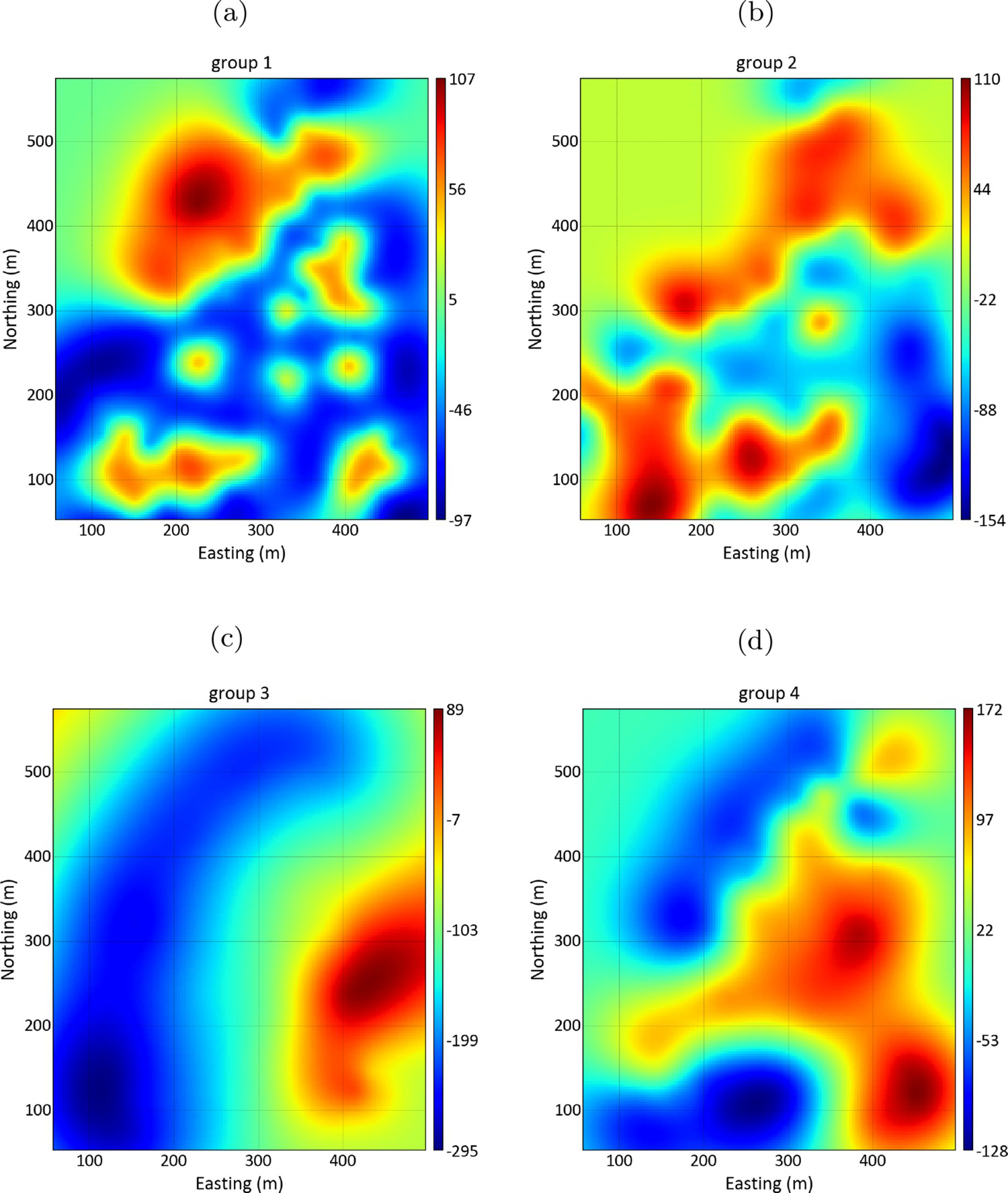

3.5 Boundary simulation

Geological model uncertainty can be assessed by simulating the contacts, for each group, and thus constructing different geological model realisations. In order to obtain contacts that are smooth and continuous, simulated and interpolated values are compared inside the uncertainty zone. If the interpolated value is less than the simulated value, the location is classified with the indicator 1, and if the value is larger, the location is classified with the indicator 0. Locations where interpolation is equal to simulation are the contacts, as shown in Figure 7.

Figure 7

Schematic illustration showing how the contacts are simulated. Simulated distances are compared with interpolated distances inside the uncertainty zone, defined between and .

For the simulation to be performed uniformly between and , the standard normal value, , is simulated and transformed by the relation: (3) in which is the value of the simulated distance function, is the standard normal value of a non-conditional simulation and represents the value of the cumulative standard distribution (cdf) corresponding to , which lies between 0 and 1. To ensure that the values belong to the determined uncertainty zone, [ , ], the values are multiplied by and subtracted from C.

Then the standard deviation,

can be simulated using unconditional sequential Gaussian simulation. The algorithm works as follows:

Algorithm 2: Unconditional sequential simulation

1.Define a random path through the grid nodes

for i in (K–1) do

1. Search for previously simulated data

if number of previously simulated data != 0 then

1. Build and solve kriging system

2. Sample the conditional distribution defined by kriging mean and variance

else

1. Sample from a standard Gaussian distribution

end

2. Assign sampled value to the model node and include the simulated node to the previously simulated data ensemble

end

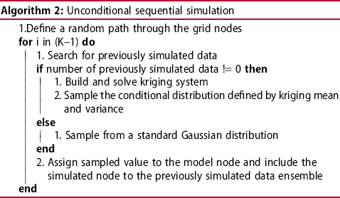
Figure 8 presents, one realisation out of 10, of the simulated Gaussian values inside the uncertainty zone for each group.

Figure 8

Simulated Gaussian values, inside the uncertainty zone, for each group: (a) simulated Gaussian values for group 1; (b) simulated Gaussian values for group 2; (c) simulated Gaussian values for group 3; (d) simulated Gaussian values for group 4.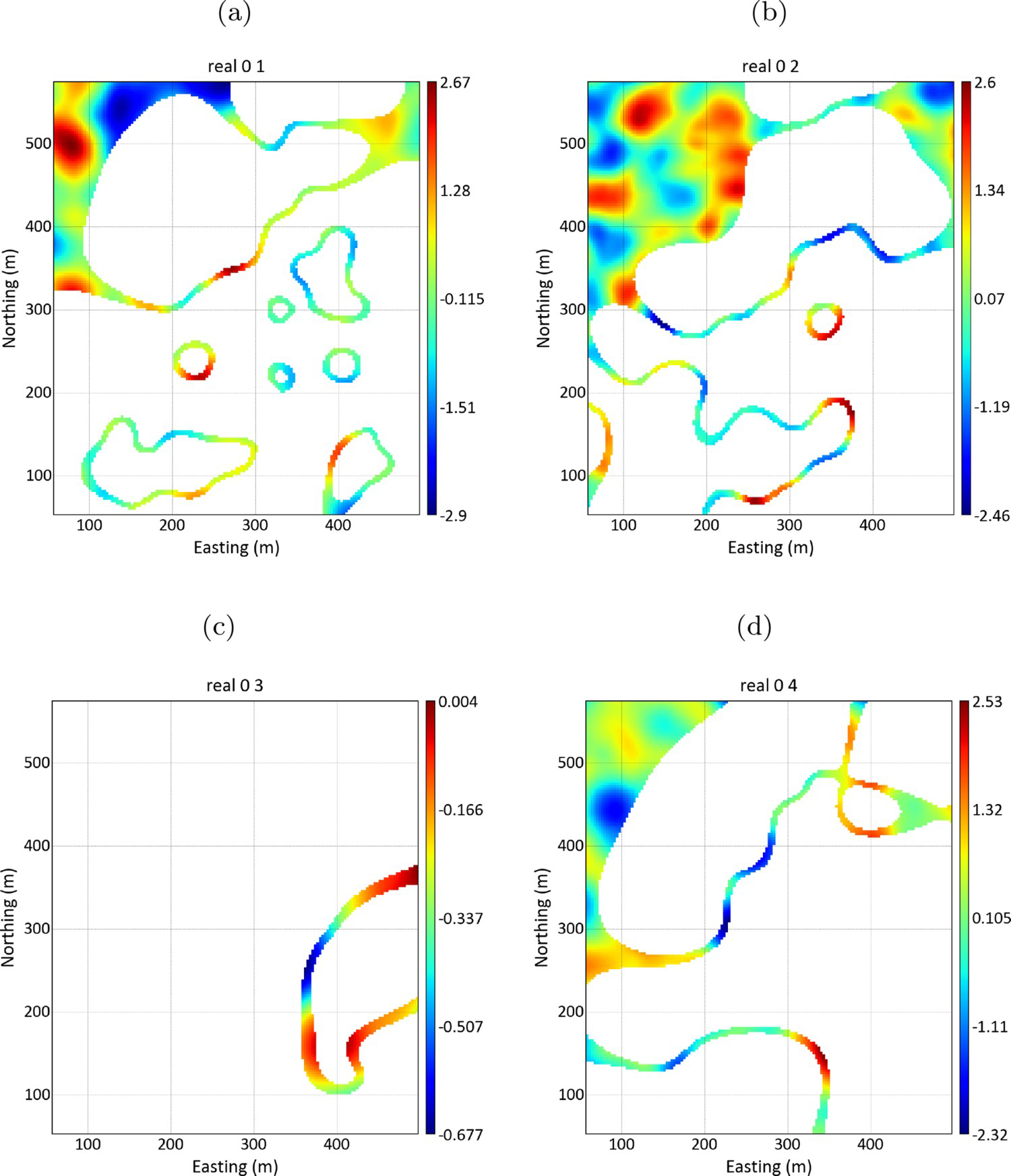

As a contact is being simulated, it is recommended to use a Gaussian variogram for non-conditional simulation, as it allows short-range continuity to be reproduced (Wilde and Deutsch 2012). Also, it is recommended to use a small nugget effect to avoid calculation instabilities. The range of the Gaussian variogram used in simulation determines the contact's characteristics. Smaller ranges generate rougher contacts, while larger ranges generate smoother contacts.

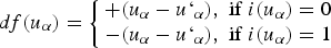
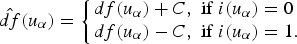
The classification of the location u as indicator 1 or 0 is performed by comparing the interpolated values with the simulated values according to the relation: (4) Figure 9 shows one realisation of simulated boundaries for each group.

Figure 9

Boundary simulation for each group: (a) boundary simulation for group 1; (b) boundary simulation for group 2; (c) boundary simulation for group 3 and (d) boundary simulation for group 4.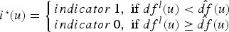

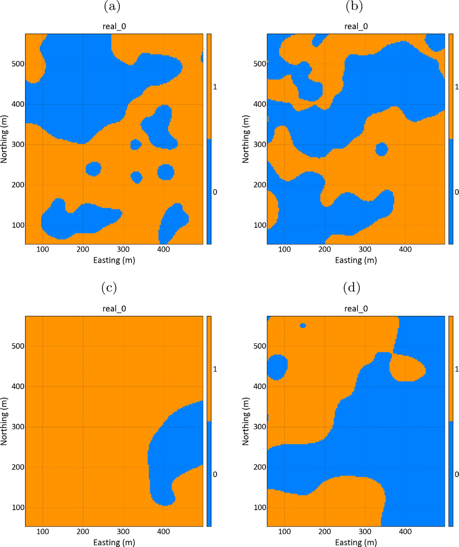
Realisations for each group must be overlaid to generate a realisation for the geological model. The corresponding category should now be assigned to each grid node according to the hierarchisation rules of Figure 4. For example, Kimmeridgian is assigned to a grid node if two conditions were satisfied: the block belongs to the group 1 region, classified with indicator 1, and belongs to the region classified with indicator 1 in the group 2. Similarly, Argovian is assigned to a grid node if three conditions were satisfied: the block belongs to the group 1 region, classified with indicator 0, the block belongs to the region classified with indicator 1 in the group 3, and the block belong to the region classified with indicator 1 in group 4.

Figure 10 shows 4, out of 10 realisations, for the geologic model. An animation of the 10 realisations can be seen here.

Figure 10

Geological model realisations: (a) realisation 0; (b) realisation 1; (c) realisation 2 and (d) realisation 3.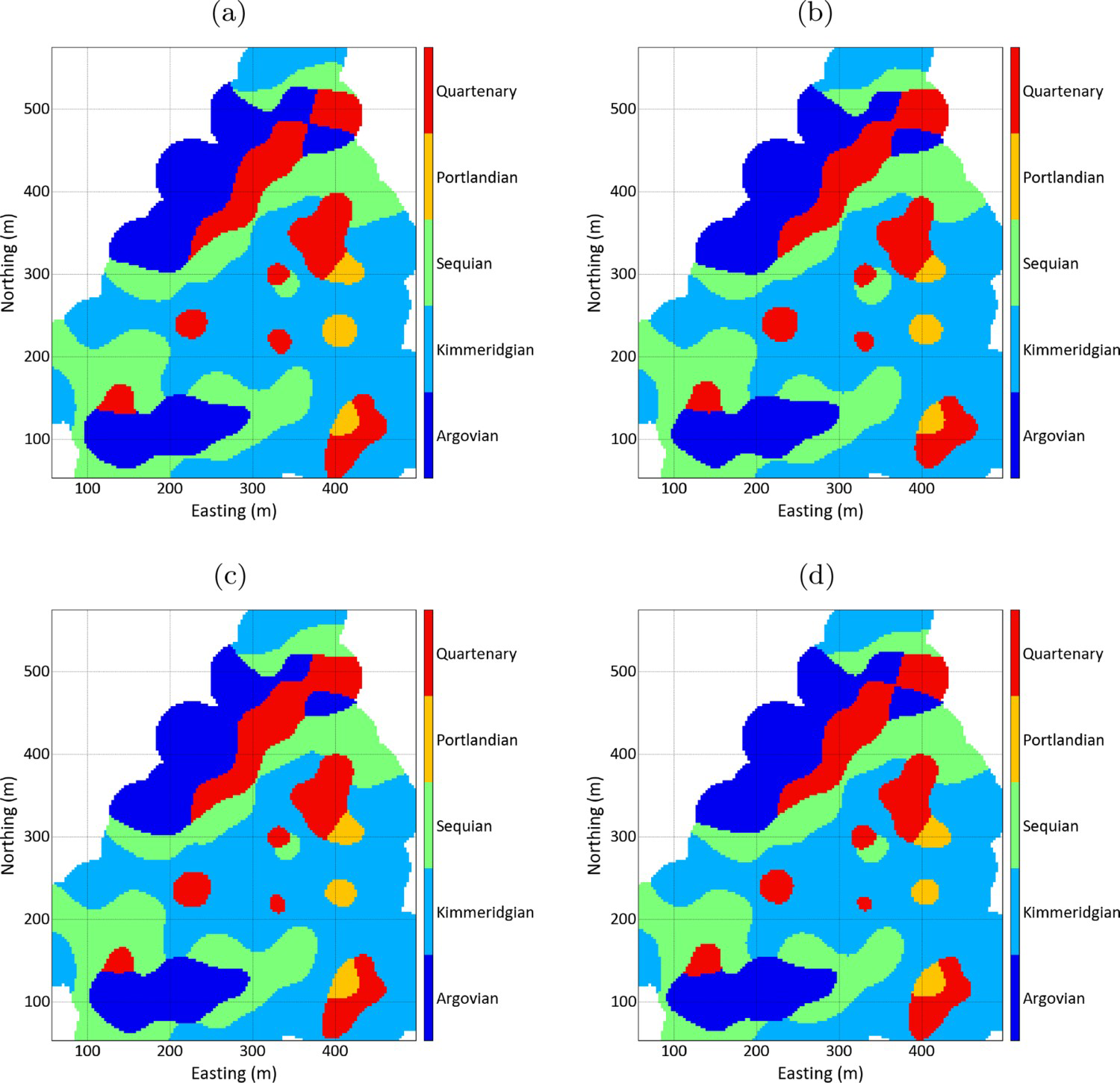

4 Case study

This case study was performed on a porphyry copper deposit to demonstrate the proposed methodology. The mineral deposit consists of 5 geological domains mapped using data from 91 drill holes, that were composited in 15 m, which leads to 3276 quasi point support samples. Three domains are intrusive rocks, one domain is oxidised rocks, and the last one is sulfide rocks. Figure 11 shows a perspective view from the composited drillings. Dark blue samples represent category 1, sulfide rocks; light blue represents category 2, oxidised rocks; and green, yellow and red represent categories 3, 4 and 5 of intrusive rocks, respectively.

Figure 11

Perspective view for the dataset at point support depicting the five categories. Axes are in metres.

The proposed grouping algorithm was applied to a proto model created using signed distances from the porphy copper data in a 50×50×30 m grid. As result, the hierarchy rule presented in Figure 12 is generated. The samples of each data sets are shown in Figure 13.

Figure 12

Hierarchy rule for the case study dataset defined by the proposed algorithm.

Figure 13

Perspective view for the group datasets at point support. Axes are in metres: (a) Group 1, (b) Group 2, (c) Group 3, (d) Group 4.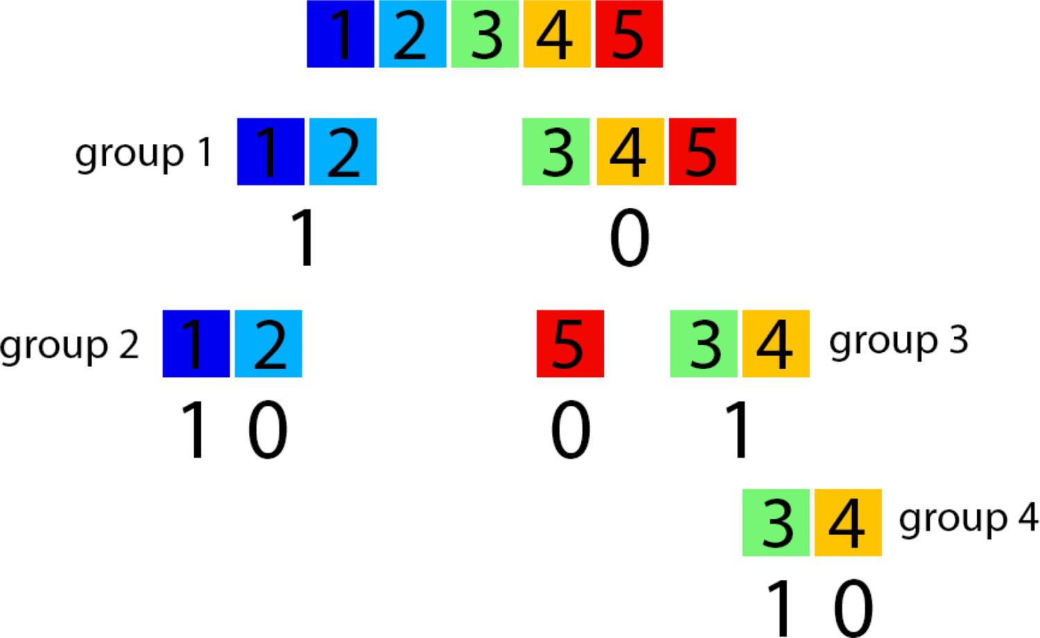

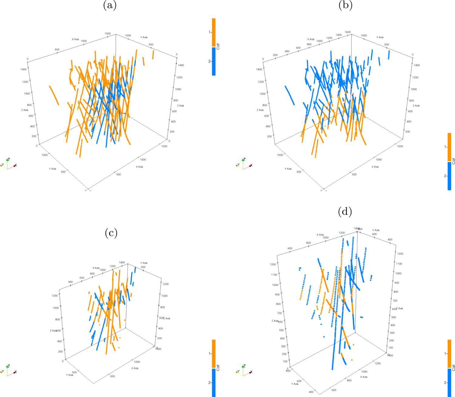
Figure 14 shows the indicator variograms for each group. For groups 1, 3 and 4 an omnidirectional variogram was calculated and modelled. While for group 2 an omnihorizontal (in blue) and vertical (in red) variograms were calculated and modelled.

Figure 14

Indicator variograms for each group: (a) omnidirectional indicator variogram for group 1; (b) omnihorizontal indicator variogram for group 2 in blue and vertical indicator variogram for group 2 in red; (c) omnidirectional indicator variogram for group 3; (d) omnidirectional indicator variogram for group 4.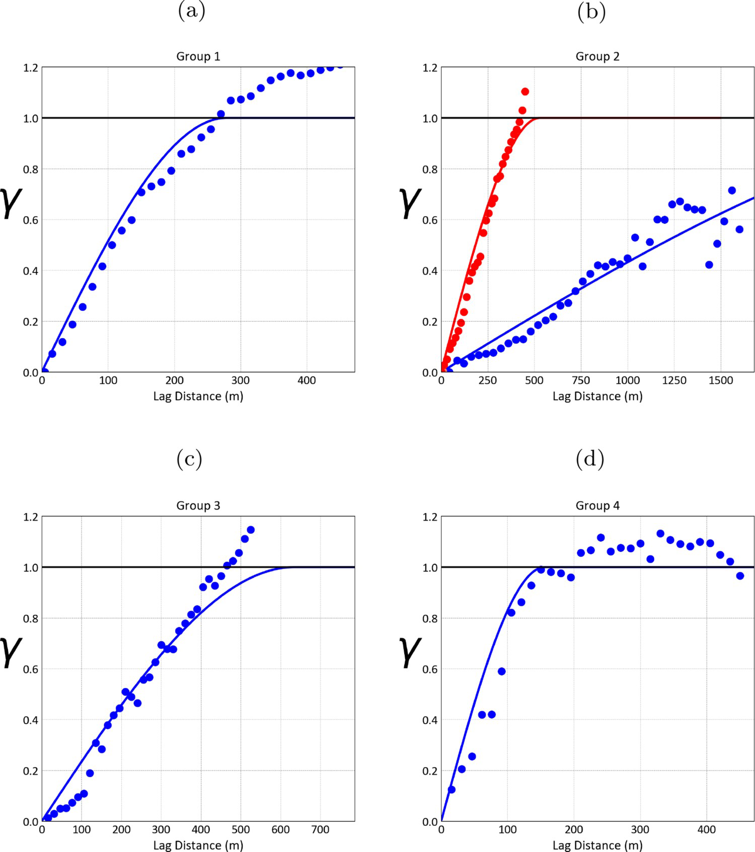

Parameter C calibration was performed with 20 random jackknife data sets drawn from each group by removing 10% of drill holes on each run, and with 30 random C parameters from zero to a determined range in metres for each group. The C calibration should be performed for a variety of jackknife subsets to ensure that the calibration is robust (Wilde and Deutsch 2012). Results are shown in Figure 15.

Figure 15

Parameter C calibration by jackknife: (a) Group 1, (b) Group 2, (c) Group 3, (d) Group 4.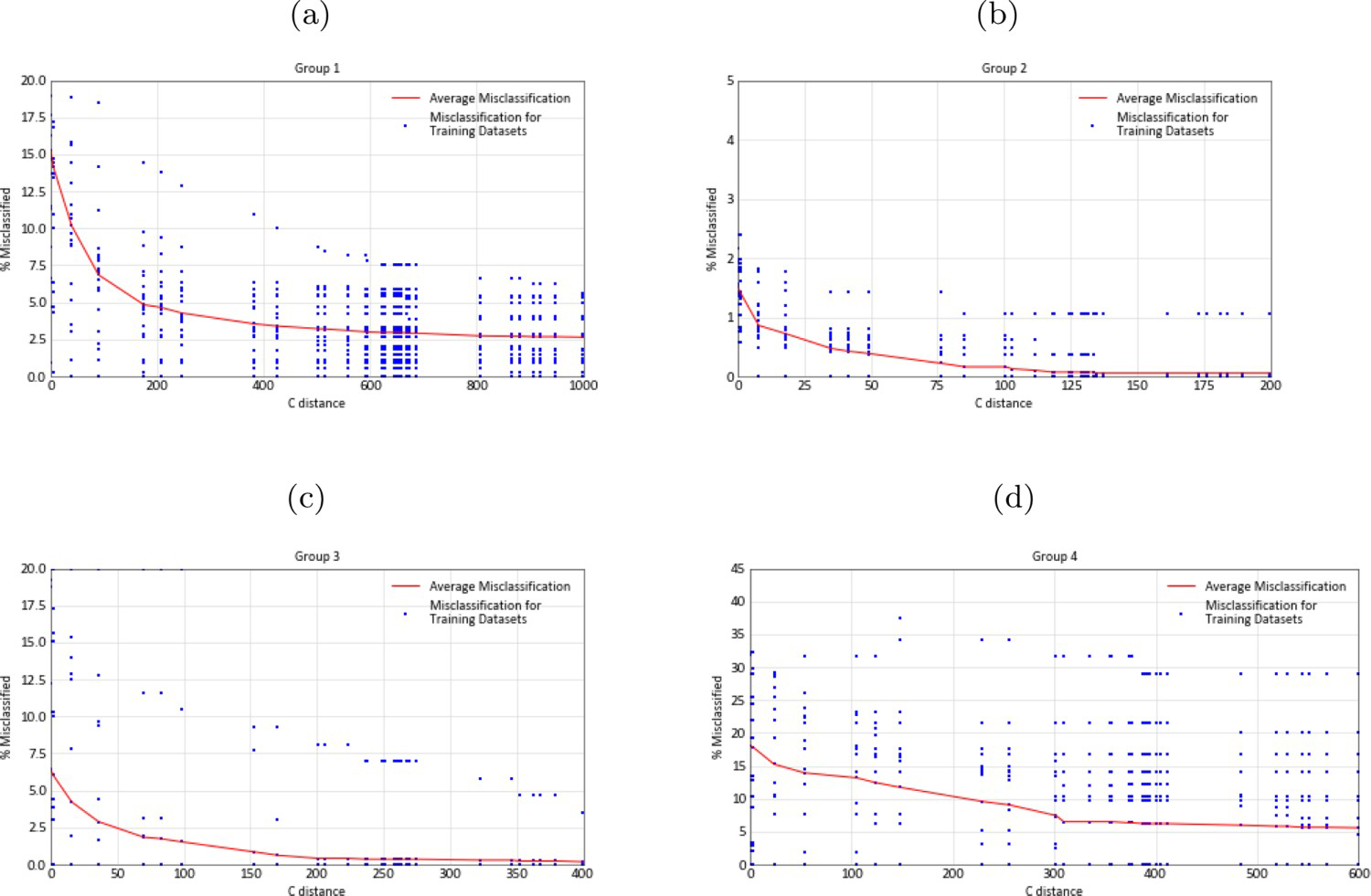

The guideline to choose a C parameter for each group from the misclassification in Figure 15 is to consider an acceptable misclassification rate (Martin and Boisvert 2017). Manchuck and Deutsch (2015) suggests 2.5% is an acceptable rate for the tabular deposit modelled in that study. Martin and Boisvert (2017) chose 3.9% as the misclassification rate for one of the domains of a porphyry copper deposit which corresponded to the point where the misclassification curve levels out. C depends on deposit and data configuration and it is small if the geological shapes are well constrained by the data configuration. For these reasons, reasonably values for C parameters were chosen for each group based on the calibration results, the deposit type and data configuration.

Chosen values were 5%, 0.5%, 2.5% and 10% misclassification rates for groups 1, 2, 3 and 4 respectively, which corresponds to 170 m, 30 m, 50 m and 200 m C parameter values. The choice of parameter C from jackknife calibration is subjective, however, the calibration assists the geomodeller in choosing a suitable value for the parameter. A value of C should not be chosen in the region where the curve becomes horizontal. Besides that, the uncertainty bandwidth cannot be greater than the drill hole spacing (Rossi and Deutsch 2013).

Distance functions calculated for each group data set were modified with the chosen parameter C, adding C to samples coded as 0 and subtracting C from samples coded as 1. Modified distances for each group should then be interpolated. Radial basis functions were chosen to interpolate the distance function to a grid with block dimensions of 25×25×15 m. The RBF kernel is Gaussian with 0.001% nugget effect to avoid instabilities in the matrices. The support distance is the range of the indicator variogram for each group and the anisotropy ratios of each group were also considered.

The uncertainty zone is obtained from interpolated models, truncating it between and . Non-conditional simulations are performed in this region, and each realisation result is standardised between and according to Equation (3). Ten realisations were generated for each group by simulating and comparing to interpolated values inside each uncertainty zone. The same indicator variograms Gaussian equivalents used for each group RBF interpolation were used for simulation.

Realisations for each group must be overlaid respecting Figure 12 hierarchisation rule to generate a realisation for the geological model. In addition, categories are merged respecting the realisation number. Realisation 2 obtained in each group's simulation is used to construct realisation 2 of the hierarchical geological model.

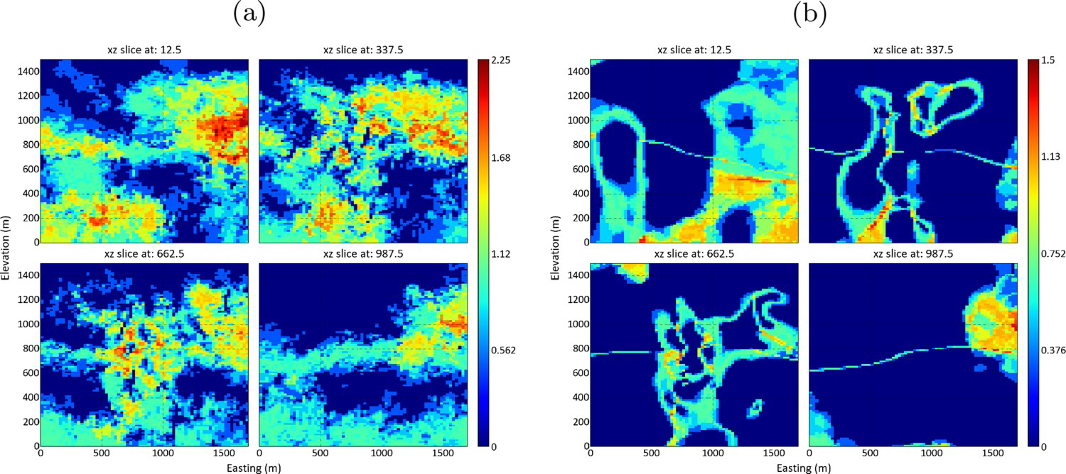
Figure 16 shows a vertical and a horizontal section for four different geological model realisations together with the point sample data. An animation of the 10 realisations in XZ sections can be seen here.

Figure 16

Geological model realisations. Axes are in metres. (a) Realisation 0; (b) Realisation 1; (c) Realisation 2; (d) Realisation 3.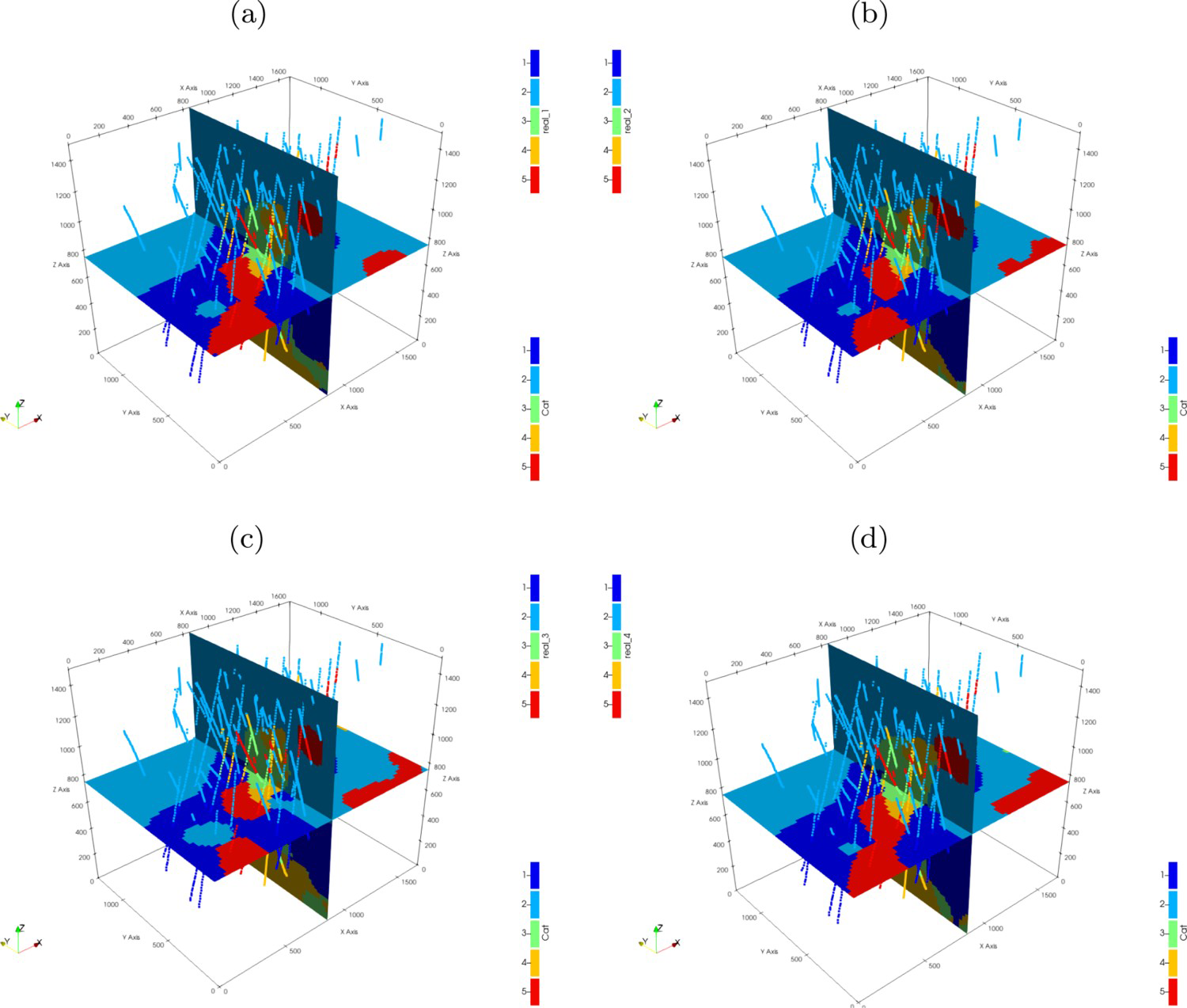

5 Discussion

In the mining industry, deterministic geological models are widely used. However, these models do not permit an uncertainty assessment in volumes and tonnes. The geometry of the geological domains directly affects the assessment of mineral resources since it determines the volumes of ore and waste available. Thus the impact is significant in the estimation of the ore tonnage, leading to biased estimations, errors in mine planning, unexpected costs in the operation and deviations in the expected revenues (Srivastava 2005).

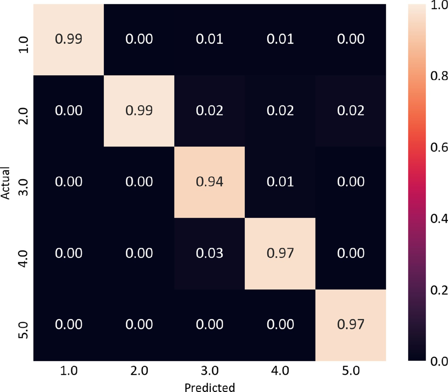
One of the traditionally used technique to model geobodies and assess its uncertainty in the presence of multiple categories, which also rely only on composited drill holes X, Y and Z coordinates and the rock type property, is sequential indicator simulation (SISIM). SISIM was applied to the same dataset in order to compare the results with the proposed methodology. Indicator variograms for the five categories were calculated and modelled, and the indicators were simulated to the same grid as hierarchical boundary simulation was performed. Figure 17(a) shows the same 4 vertical sections along XZ comparing one realisation of SISIM with the proposed methodology. SISIM generates a model with a typical ‘salt and pepper’ texture and noisy patterns, which is not geologically realistic. Boundary simulation (Figure 17b) generates continuous boundaries, that honour the data, as shown by the confusion matrix in Figure 19, and are geologically realistic. Besides that, only 4 indicator variograms, one for each group, must be calculated and modelled, against 5 variograms for SISIM. Since RBF is a global interpolator, search neighbourhood parameters must not be set, unlike SISIM. As drawbacks, the algorithm has no mechanism for respecting the proportions and to reproduce the spatial continuity of each category, although this can be worked around by iteratively changing the parameters and checking the results.

Figure 17

Equidistant sections in XZ comparing one realisation of SISIM to the one realisation of the proposed methodology: (a) SISIM section and (b) proposed methodology sections.

Figure 19

Confusion matrix showing the average of the proportion of blocks that reproduce the closest samples among all the realisations for all categories in the dataset.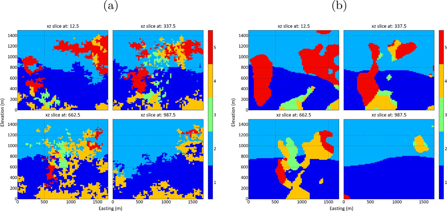

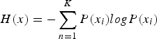
One quantitative way of assessing the uncertainty of 3D geological models is using the information entropy (Shannon 2001), calculated as Equation 5, it has been applied in geoscience as a quality measurement of geological models (Yang et al. 2019). Where K are the categories in the mineral deposit and is probability that a given block belongs to category i. (5) Figure 18 shows the information entropy calculated for SISIM and the proposed methodology. As expected, in the proposed methodology the highest values for information entropy are around the contacts, unlike SISIM, where high entropy values are scattered in space. Most uncertainty lies in areas where multiple categories have a high probability of occurrence.

Figure 18

Equidistant sections in XZ comparing SISIM to the proposed methodology: (a) SISIM entropy section and (b) proposed methodology entropy section.

It is worth mentioning that the main disadvantage of the method consists of determining the rules for the contacts hierarchy. The proposed algorithm automates the process, however, the resolution of the proto model grid and the method used to create the proto model can produce different groupings. The hierarchy between categories can be determined chronologically by a geomodeller. However, this choice depends on the knowledge about the mineral deposit and the experience of the geomodeller. It can also be determined in an arbitrary way, which can lead to subjective, irreproducible and not auditable geological models.

5.1 Influence of parameters

The simulation grid parameters may be predetermined by the engineering requirements for a certain project. However, the grid definitions for the geological model are not required to match those for the numerical modelling; the most important consideration is the ability to resolve the smallest geological features of interest (Martin and Boisvert 2017). Parameter C and grid resolution must be compatible, if C parameter is greater than the cell dimensions the uncertainty zone may have few blocks or none at all.

The interpolation variogram parameters, namely, range, anisotropy and nugget effect, control the shape and volume of different categories. There is a close relation between the variogram used for interpolating of each group and the C parameters. The same value for C can lead to a larger uncertainty zone if the range of the variogram increases.

Contacts behaviour is controlled by the variogram used in the unconditional simulation, smaller ranges and higher nugget effects generates rough and discontinuous boundaries, conversely long ranges and small nugget effects generate smooth and continuous boundaries.

The magnitude of the uncertainty can be controlled by the C parameter, which defines the uncertainty bandwidth. It can be calibrated from the existing data or determined by an expert, based on knowledge about the deposit, the width of uncertainty must be neither too large nor too small, the true boundary must exist at some location within the uncertainty zone. The volume variation of each lithology depends directly on the C parameter defined for each group. Figure 20 shows the entropy of information calculated for the Swiss Jura example with different values for C. Figure 20(a) shows the base case, where the C values for all groups are equal to 12 m, Figure 20(b) shows the entropy of information for C values equals to 60 m to all groups, the uncertainty bandwidth is larger than the base case. Finally, Figure 20(c) shows a case where C parameter is equal to 12 m for groups 1, 2 and 3 and 60 m for group 4. Since group 4 represents the contact between Argovian and quartenary, the uncertainty zone is larger around these contacts than the others.

Figure 20

Effect of the C parameter: (a) C for group 1: 12m; C for group 2: 12m; C for group 3: 12m; C for group 4: 12m; (b) C for group 1: 60m; C for group 2: 60m; C for group 3: 60m; C for group 4: 60m; (c) C for group 1: 12m; C for group 2: 12m; C for group 3: 12m; C for group 4: 60m.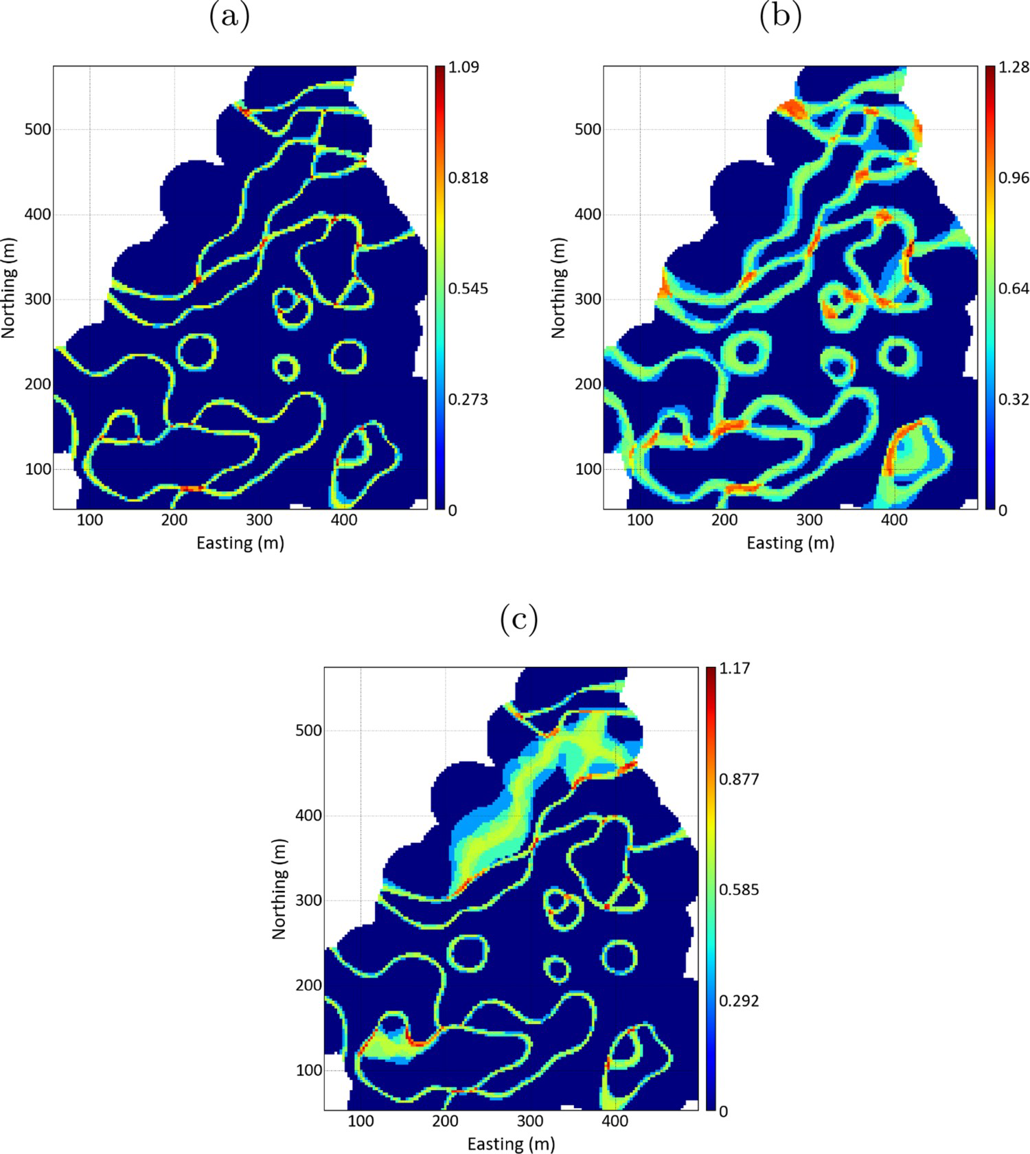

6 Conclusion

Geostatistical methods require the prior delimitation of stationary domains for modelling the mineral deposit. There is uncertainty in determining limits between these domains. Methods available in the literature for contacts simulation using signed distances and relying on the C parameter accounts for one lithology at time, in the presence of multiple lithologies the workflow must be applied for each category one by one. This process leads to models that overlap or have no classified blocks to any of the categories in some realisations. The proposed methodology deals with this problem and reduces the geomodeller effort.

The proposed method was demonstrated in a case study conducted on a porphyry copper deposit, in which the geological uncertainty was assessed. Models generated by the proposed method do not show much noise, and the method leads to continuous contacts between domains while the volume variation and contacts characteristics can be controlled by the parameters.

Although the method produces realistic models in a straightforward manner, the calibration and choice of parameter C still depend on subjective choices. Different geomodellers can define a different C value from the same calibration. For this reason, we suggest, as future work, an objective methodology for the calibration and determination of C.

In addition, the grouping can also be subjective, since the proposed algorithm depends on a proto model that can have variable grid resolution and creation method. However, using the same proto model, the same C parameters and the same seed for the simulation make the models replicable.

Footnotes

Acknowledgments

The authors would like to thank the National Council for Scientific and Technological Development (CNPq) for supporting the Mineral Exploration and Mining Planning Research Unit (LPM) at the Universidade Federal do Rio Grande do Sul. The authors also thank the anonymous reviewers for their constructive comments, which helped us to improve the quality of our paper.

Disclosure statement

No potential conflict of interest was reported by the author(s).

References

Alabert

1987. Stochastic imaging of spatial distributions using hard and soft information [PhD thesis]. Stanford University Press.

Armstrong

, Galli

, Beucher

, Loc'h

, Renard

, Doligez

, Eschard

, Geffroy

(2011). Plurigaussian simulations in geosciences. Berlin: Springer Science & Business Media Sage UK: London, England.

Boucher

2009. Considering complex training images with search tree partitioning. Comput Geosci. 35(6):1151–1158.

Calcagno

, Chilès

J-P

, Courrioux

, Guillen

2008. Geological modelling from field data and geological knowledge: part i. modelling method coupling 3d potential-field interpolation and geological rules. Phys Earth Planetary Interiors. 171(1-4):147–157.

Caumon

, Tertois

A-L

, Zhang

2007. Elements for stochastic structural perturbation of stratigraphic models. In: EAGE Conference on Petroleum Geostatistics, European Association of Geoscientists & Engineers, Cascais, September. p. cp–32.

Chilès

J-P

, Aug

, Guillen

, Lees

2004. Modelling the geometry of geological units and its uncertainty in 3d from structural data: the potential-field method. In: Proceedings of International Symposium on Orebody Modelling and Strategic Mine Planning, vol. 22, Perth, Australia. p. 24.

Cowan

, Beatson

, Fright

, McLennan

, Mitchell

2002. Rapid geological modelling. In: Applied Structural Geology for Mineral Exploration and Mining, International Symposium, Kalgoorlie, September. p. 23–25.

Cowan

, Beatson

, Ross

, Fright

, McLennan

, Evans

, Carr

, Lane

, Bright

, Gillman

, Oshust

, Titley

2003. Practical implicit geological modelling. In: 5th International Mining Geology Conference, AusIMM Publication Series, Victoria, November. p. 17–19.

de la Varga

, Schaaf

, Wellmann

2019. Gempy 1.0: open-source stochastic geological modeling and inversion. Geoscientific Model Development.

10.

Deutsch

CV.

2006. A sequential indicator simulation program for categorical variables with point and block data: blocksis. Comput Geosci. 32(10):1669–1681.

11.

Gonçalves

ÍG

, Kumaira

, Guadagnin

2017. A machine learning approach to the potential-field method for implicit modeling of geological structures. Comput Geosci. 103:173–182.

12.

Goovaerts

1997. Geostatistics for natural resources evaluation. Oxford: Oxford University Press Sage UK: London, England.

13.

Guardiano

, Srivastava

RM.

1993. Multivariate geostatistics: beyond bivariate moments. In: Geostatistics Troia'92, Springer, Troia. p. 133–144.

14.

Karpekov

, Deutsch

2016. A review of boundary modeling and one way of selecting the C parameter to model boundaries with uncertainty. Center for Computational Geostatistics Annual Report, Alberta. p. 18.

15.

Lajaunie

, Courrioux

, Manuel

1997. Foliation fields and 3d cartography in geology: principles of a method based on potential interpolation. Math Geol. 29(4):571–584.

16.

Lillah

, Boisvert

JB.

2013. Stochastic distance based geological boundary modeling with curvilinear features. Math Geosci. 45(6):651–665.

17.

Lindsay

, Aillères

, Jessell

, de Kemp

, Betts

PG.

2012. Locating and quantifying geological uncertainty in three-dimensional models: analysis of the Gippsland basin, Southeastern Australia. Tectonophysics. 546:10–27.

18.

Lorensen

, Cline

HE.

1987. Marching cubes: a high resolution 3d surface construction algorithm. In: ACM Siggraph Computer Graphics, vol. 21, ACM, Anaheim, August. p. 163–169.

19.

Manchuck

, Deutsch

2015. Geometric modeling of irregular tabular deposits. Center for Computational Geostatistics Annual Report, Alberta. p. 17.

20.

Martin

, Boisvert

2017. Implicit modeling. Alberta: University of Alberta – CCG, Guidebook volume 22.

21.

Matheron

, Beucher

, De Fouquet

, Galli

, Guerillot

, Ravenne

1987. Conditional simulation of the geometry of fluvio-deltaic reservoirs. In: SPE Annual Technical Conference and Exhibition, Society of Petroleum Engineers, Dallas, September.

22.

McLennan

, Deutsch

CV.

2006. Implicit boundary modeling (boundism). Center for Computational Geostatistics Annual Report, Alberta.

23.

Munroe

, Deutsch

2008. Full calibration of c and β in the framework of vein-type deposit tonnage uncertainty. In: Center for Computational Geostatistics Annual Report. p. 10.

24.

Pakyuz-Charrier

, Lindsay

, Ogarko

, Giraud

JECD

, Jessell

MW.

2018. Monte Carlo simulations for uncertainty estimation in 3d geological modeling, a guide for disturbance distribution selection and parameterization. Solid Earth. 9:385–402.

25.

Pyrcz

, Deutsch

CV.

2014. Geostatistical reservoir modeling. Oxford: Oxford University Press Sage UK: London, England.

26.

Rossi

, Deutsch

2013. Mineral resource estimation. Berlin: Springer Science & Business Media Sage UK: London, England.

27.

Shannon

CE.

2001. A mathematical theory of communication. ACM SIGMOBILE Mobile Comput Commun Rev. 5(1):3–55.

28.

Silva

2015. Enhanced geologic modeling with data-driven training images for improved resources and recoverable reserves [PhD thesis]. University of Alberta.

29.

Silva

2018. Enhanced geologic modeling of multiple categorical variables [PhD thesis]. University of Alberta.

30.

Silva

, Deutsch

2019. Multivariate categorical modeling with hierarchical truncated pluri-gaussian simulation. Math Geosci. 51(5):527–552.

31.

Srivastava

2005. Probabilistic modeling of ore lens geometry: an alternative to deterministic wireframes. Math Geol. 37(5):513–544.

32.

Strebelle

2002. Conditional simulation of complex geological structures using multiple-point statistics. Math Geol. 34:1–21.

33.

Wilde

, Deutsch

2012. Kriging and simulation in presence of stationary domains: developments in boundary modeling. In: Geostatistics Oslo 2012, Springer, Oslo, June. p. 289–300.

34.

Yang

, Hyde

, Grujic

, Scheidt

, Caers

2019. Assessing and visualizing uncertainty of 3d geological surfaces using level sets with stochastic motion. Comput Geosci. 122:54–67.

Boundary simulation – a hierarchical approach for multiple categories

Abstract

Keywords

1 Introduction

2 Background

3 Methodology

3.3 Signed distances calculation

(1) Calculated distances should be modified by the C parameter, for each group its value is added to samples coded as 0 and subtracted from samples coded as 1, according to the relation: (2) 3.4 Distance function interpolation

Footnotes

Acknowledgments

Disclosure statement

References

(1) Calculated distances should be modified by the C parameter, for each group its value is added to samples coded as 0 and subtracted from samples coded as 1, according to the relation: (2)
3.4 Distance function interpolation