Accurate Differentiation of Carotenoid Pigments Using Flight Representative Raman Spectrometers

Abstract

Raman spectrometers will be utilized on two Mars rover missions, ExoMars and Mars 2020, in the near future, to search for evidence of life and habitable geological niches on Mars. Carotenoid pigments are recognized target biomarkers, and as they are highly active in Raman spectroscopy, they can be readily used to characterize the capabilities of space representative instrumentation. As part of the preparatory work being performed for the ExoMars mission, a gypsum crust colonized by microorganisms was interrogated with commercial portable Raman instruments and a flight representative Raman laser spectrometer. Four separate layers, each exhibiting different coloration resulting from specific halophilic microorganism activities within the gypsum crust, were studied by using two excitation wavelengths: 532 and 785 nm. Raman or fluorescence data were readily obtained during the present study. Gypsum, the main constituent of the crust, was detected with both excitation wavelengths, while the resonance Raman signal associated with carotenoid pigments was only detected with a 532 nm excitation wavelength. The fluorescence originating from bacteriochlorophyll a was found to overwhelm the Raman signal for the layer colonized by sulfur bacteria when interrogated with a 785 nm excitation wavelength. Finally, it was demonstrated that portable instruments and the prototype were capable of detecting a statistically significant difference in band positions of carotenoid signals between the sample layers. Key Words: Gypsum—Raman spectrometers—Carotenoids—ExoMars—Mars exploration—Band position shift. Astrobiology 17, 351–362.

1. Introduction

In 2018, the ExoMars rover (part of the ESA and Roscosmos ExoMars mission) will commence its journey to Mars in a dedicated search for extinct or extant life signatures (ExoMars mission, 2015). On board, it will carry a Raman spectrometer that will be used to analyze crushed rock specimens retrieved from the surface and subsurface of the planet with a drill that is able to sample down to a depth of about 2 m (Rull et al., 2011; Lopez-Reyes et al., 2013; Hutchinson et al., 2014). Two years later, the Mars 2020 rover (a NASA mission with similar objectives to ExoMars) is also due to be launched and will carry two separate Raman spectrometers on board (NASA Mars 2020, 2014). In preparation for these planetary exploration missions, the ability of Raman spectroscopy techniques to analyze the extremophilic colonizations of geological substrates has gained importance.

One of the key advantages of Raman spectroscopy for planetary exploration is that a geological sample can be characterized in terms of both mineralogy and organic chemistry at the same time. The scattering light emitted by inorganic molecules (constituting the geological matrix) is typically observed at Raman shifts ranging from 10 to 1100 cm⁻¹, while the organic molecules exhibit Raman signal typically between 1000 and 3400 cm⁻¹. The contribution of inorganic and organic molecules can then often be distinguished in one Raman spectrum (Jorge Villar and Edwards, 2006). However, the Raman scattering cross section of organic molecules is lower than the cross section of inorganic molecules, meaning that inorganic compounds scatter more Raman light than organic materials when present in equal concentration (Edwards et al., 2013). When a sample of biogeological interest is interrogated, the concentration of organic molecules is usually much lower than the concentration of inorganic molecules; consequently, the signal associated with the organic components is often not observed (the concentration being below the sensitivity limit of the instrument). In particular cases, however, when the selected excitation wavelength can promote electronic transitions within an organic molecule (often with UV and visible light), a coupling between the excitation photons and the electrons of the chromophore (part of the molecule which absorbs the light and is promoted to a higher electronic level of energy) occurs, and the scattered Raman signal is enhanced by a factor 10³ to 10⁵, which is known as resonance Raman (Ferraro et al., 2003). Candidate molecules expected to give resonance Raman are colored and often referred to as pigments, among them carotenoids.

Carotenoids are organic molecules that comprise a long conjugated and methylated carbon chain whose length and extremities vary (some examples are given in Fig. 1) (Marshall et al., 2007; Edwards et al., 2013). They are highly valuable for extremophilic microorganisms exposed to high insolation because carotenoids absorb green visible light (450–550 nm, which is not absorbed by chlorophyll) and prevent the formation of highly damaging singlet dioxygen by quenching triplet states of chlorophylls (Telfer, 2005). When they absorb visible light, their delocalized π electrons (distributed along the conjugated carbon chain) are promoted to a higher level of electronic energy (transition π-π*). Under resonance conditions, three bands are mainly observed for carotenoids. The first band, strong in terms of intensity, is observed between 1500 and 1550 cm⁻¹ and is due to the stretching of the C═C bonds of the polyene chain (band ν₁). The second band, presenting a similar level of intensity, is located between 1100 and 1200 cm⁻¹ and arises from the stretching of the C–C bonds of the conjugated carbon chain (band ν₂). The last band, found between 990 and 1050 cm⁻¹, is weaker in intensity and arises from the rocking of the pendant methyl groups attached to the polyene chain (band ν₃) (Marshall et al., 2007; Edwards et al., 2013).

FIG. 1.

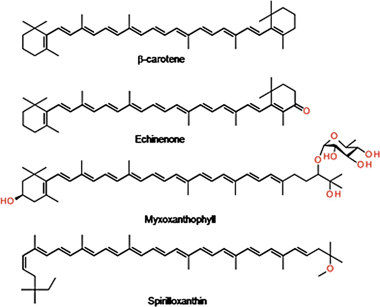
Structure of carotenoids excreted by cyanobacteria and purple sulfur bacteria found in the benthic sulfate crust of saltern ponds near Eilat, Israel. The polyene chain of carbon atoms is indicated in bold.

Over a decade ago, the Mars Exploration Rovers, Spirit and Opportunity, confirmed the presence of evaporitic minerals on the martian surface (Gendrin et al., 2005; Grotzinger et al., 2014). On Earth, analogous hypersaline environments, such as the saltern ponds near Eilat, Israel, have been known to harbor halophilic microorganisms (Oren et al., 2009). Material from these hypersaline ecosystems provides an ideal way of measuring the detectability and discernibility of biomarkers, under Mars-like conditions, when using flight representative Raman instrumentation.

The gypsum crust on the bottom of these evaporation ponds is stratified by various types of cyanobacteria and purple sulfur bacteria (Oren et al., 2009). It has previously been reported that the strata coloration, often seen within the first few centimeters of the crust, is related to the presence of various carotenoids and other pigments produced by the microbial communities surviving within (Oren et al., 2009; Jehlička and Oren, 2013a). Portable Raman instrumentation with 532 nm excitation allows the detection of carotenoids in different colored layers even under field conditions (Jehlička and Oren, 2013b). Precise and unambiguous discrimination of individual very similar carotenoids can sometimes be challenging. For example, the purple coloring often seen in the gypsum crust can be caused by the presence of spirilloxanthin-like carotenoids (Jehlička et al., 2014; Oren, 2014a). Carotenoids such as myxoxanthophyll and echinenone have been observed within the green and orange areas of the sample (Oren et al., 2009; Jehlička and Oren, 2013b; Jehlička et al., 2014b). Some carotenoid molecules previously identified in the different layers of the Eilat benthic crusts are presented in Fig. 1. Bacterioruberin was documented as a dominant carotenoid of several Haloarchaea living in the brine (and causing the red coloration of some of the saltern ponds (Oren and Rodriguez-Valera, 2001). This carotenoid can easily be detected and discriminated by using Raman spectroscopy, even when using miniaturized instrumentation (Jehlička and Oren, 2013b; Jehlička et al., 2014a, b).

We report here a rigorous study of the gypsum crust found at the bottom of a saltern pond in Eilat using flight representative Raman spectrometers. In particular, the detectability of carotenoids present in the different colored layers was interrogated with commercial spectrometers (operating with excitation wavelengths at 532 or 785 nm) and an ExoMars RLS prototype developed at the University of Leicester. The position of the Raman bands (of the gypsum and of the carotenoids) are reported with their standard deviation, and it is demonstrated that the flight representative spectrometer is able to discriminate between the different carotenoids present in gypsum.

2. Materials and Methods

2.1. Specimens

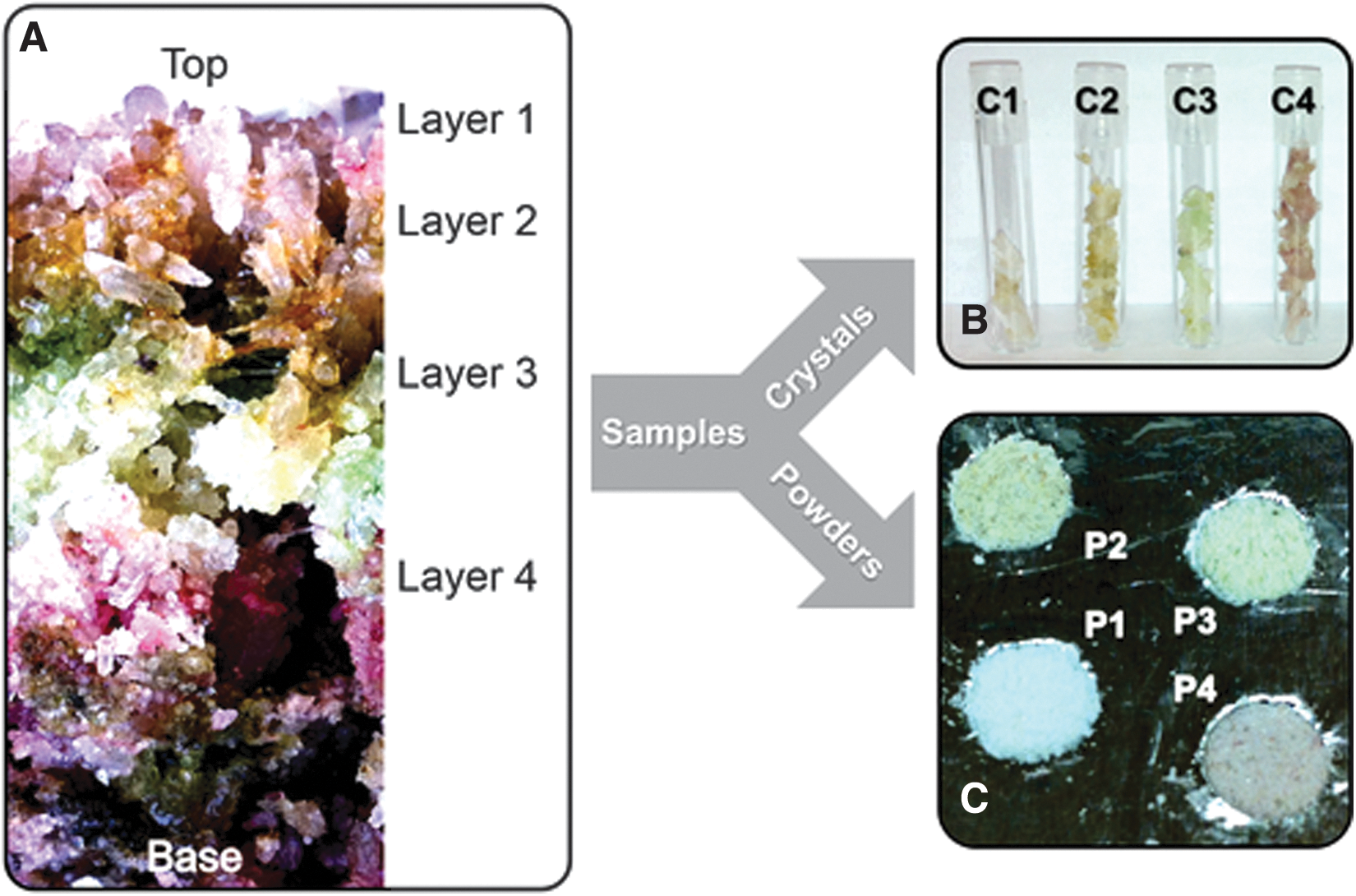
A number of samples of sulfate crust were obtained from the bottom of a salted pond in Eilat, Israel. As highlighted in Fig. 2, transverse cuts of the crust reveal colored layers arising from microorganism colonies. The upper layer is comprised of transparent gypsum crystals, which were in direct contact with the highly saline water [containing between 190 and 240 g of salts per liter (Oren et al., 2009)]. Layers 2, 3, and 4 (hosting living organisms) present yellow to orange, green, and purple coloration, respectively. Distinctive crystals from each of the four layers were isolated and labeled according to their layer of origin (C1 to C4, as shown in Fig. 2B). Small fractions of each of these samples were then crushed in an agate mortar to obtain powdered samples. Again, these samples were labeled according to their layer of origin (P1 to P4—see Fig. 2C).

FIG. 2.

(A) Transect of a sample from a salted pond in Eilat, Israel. It is colonized by several colonies of microorganisms that produce the different colored layers. (B) Individual crystals of the four top layers (namely, 1 to 4 from top to bottom) were isolated and stored in independent vials before Raman analyses were performed. (C) Some crystals were eventually crushed to obtain powders (presented here compacted into small wells for the analyses).

2.2. Raman spectroscopy

Raman spectra of the eight samples (crystals and powders) were acquired by using three separate Raman spectrometers: two portable spectrometers manufactured by DeltaNu and an RLS prototype developed at the University of Leicester as part of preparations for the ESA/Roscosmos ExoMars mission. Both portable spectrometers were calibrated before each series of measurements with polystyrene as a reference [according to the band positions published by McCreery (2001)]. The prototype was calibrated with paracetamol, and the band positions were published by Moynihan and O'Hare (2002) as a reference. The operating parameters of the portable spectrometers were similar to the flight operating modes of instruments under development for Mars exploration missions (Hutchinson et al., 2014).

The first instrument, a Raman Advantage spectrometer, utilizes a 532 nm excitation wavelength (able to irradiate the sample with a maximum power of 100 mW and a spot size of 50 μm, measured on silicon) and a thermoelectrically cooled CCD detector. Data were obtained across the 200–3400 cm⁻¹ wavenumber offset range with a spectral resolution of ∼10 cm⁻¹. The second spectrometer was a handheld portable Raman Inspector, which utilizes a 785 nm excitation wavelength (able to irradiate the sample with a maximum power of 120 mW and a spot size of 75 μm, measured on silicon) and a thermoelectrically cooled CCD detector. Data were obtained across the 200–2000 cm⁻¹ wavenumber offset range with a spectral resolution of ∼8 cm⁻¹. Care was taken to avoid any laser-induced deterioration of the samples (i.e., both the spectra and integrity of the sample were checked frequently). The third instrument, the prototype (which is similar in functionality to the proposed RLS instrument), uses a 100 mW, 532.3 nm laser, achieving a power density at the sample of 250–2100 W cm⁻². The instrument incorporates a Kaiser Optical HoloSpec spectrograph and a cooled CCD. In its baseline configuration, the spectral range is ∼200 to 4000 cm⁻¹, with a spectral resolution of ∼3 cm⁻¹.

Two separate strategies were adopted in order to obtain Raman data from the crystal and powdered samples. For the crystal samples (C1 to C4), Raman spectra were acquired from random positions on the sample surface. The Raman intensities and the spectral background were observed to fluctuate from one position to another, and the acquisition time was set accordingly (typically between 5 and 20 s with both of the 532 nm excitation wavelength and between 2 and 20 s with the 785 nm excitation line). The powdered samples (P1 to P4) were compacted into small cylindrical wells (5 mm in diameter and 1 mm deep), and a stainless steel spatula was used to smooth/flatten each of the surfaces (as shown in Fig. 2C). Raman spectra were recorded from random positions on the powder surface. The emission from those samples was observed to be more homogeneous (in terms of both background and Raman intensity levels) than the crystal samples, and the accumulation times were generally set to 15 s (in a small number of cases, the acquisition time needed to be reduced to 10 s to avoid detector saturation) with the 532 nm portable instrument. Data acquired from the powdered samples with the RLS prototype were obtained with integration times of 5–16 s. When the 785 nm excitation wavelength was used, an intense fluorescence was detected in the form of a broad feature centered at around 1400 cm⁻¹, and the acquisition time needed to be limited to between 5 and 20 s.

2.3. Data treatment

For each of the eight extracted samples (C1 to C4 and P1 to P4), 10 spectra were obtained from 10 separate (random) positions on the surface of the crystals/powders. The Raman signals associated with both gypsum and carotenoid materials are expected to be observed within the 900–1800 cm⁻¹ Raman shift range, and all the following data analysis was limited to that region.

The base line for each spectrum was estimated by iteratively evaluating a polynomial fit to the spectral background (4^th- and 7^th-order polynomials were used for the 532 and 785 nm excitation wavelengths, respectively). The first polynomial background is estimated from a reduced selection of data points (i.e., one per 10 spectral bins). Then, for each iterative step, a new polynomial is calculated to fit a new selection of data points (spectral bins are selected if the corresponding intensity is lower than the previous calculated background, plus 1% threshold of the maximum spectrum intensity). The iteration continues until a minimum is reached for the average deviation between the polynomial background and the selected data points. Raman intensities were normalized for an acquisition time of 1 s in order to compare absolute intensities for different samples and/or repeated measurements.

The band positions reported here represent the Raman shift associated with the maximum intensity observed for a particular band (which was obtained by comparing mobile averages of three data points within a given spectral range). In this study, three specific spectral regions were considered:

• 990–1020 cm⁻¹, where the δ(C–CH₃) band of carotenoids and the ν₁(SO₄ ²⁻) band of gypsum are expected;

• 1100–1200 cm⁻¹, where the ν₂(C–C) band of the carotenoids and the ν₃(SO₄ ²⁻) band of gypsum are expected;

• 1500–1550 cm⁻¹, where the ν₁(C═C) band of the carotenoids is expected.

3. Results

3.1. Data obtained with the Advantage instrument (532 nm)

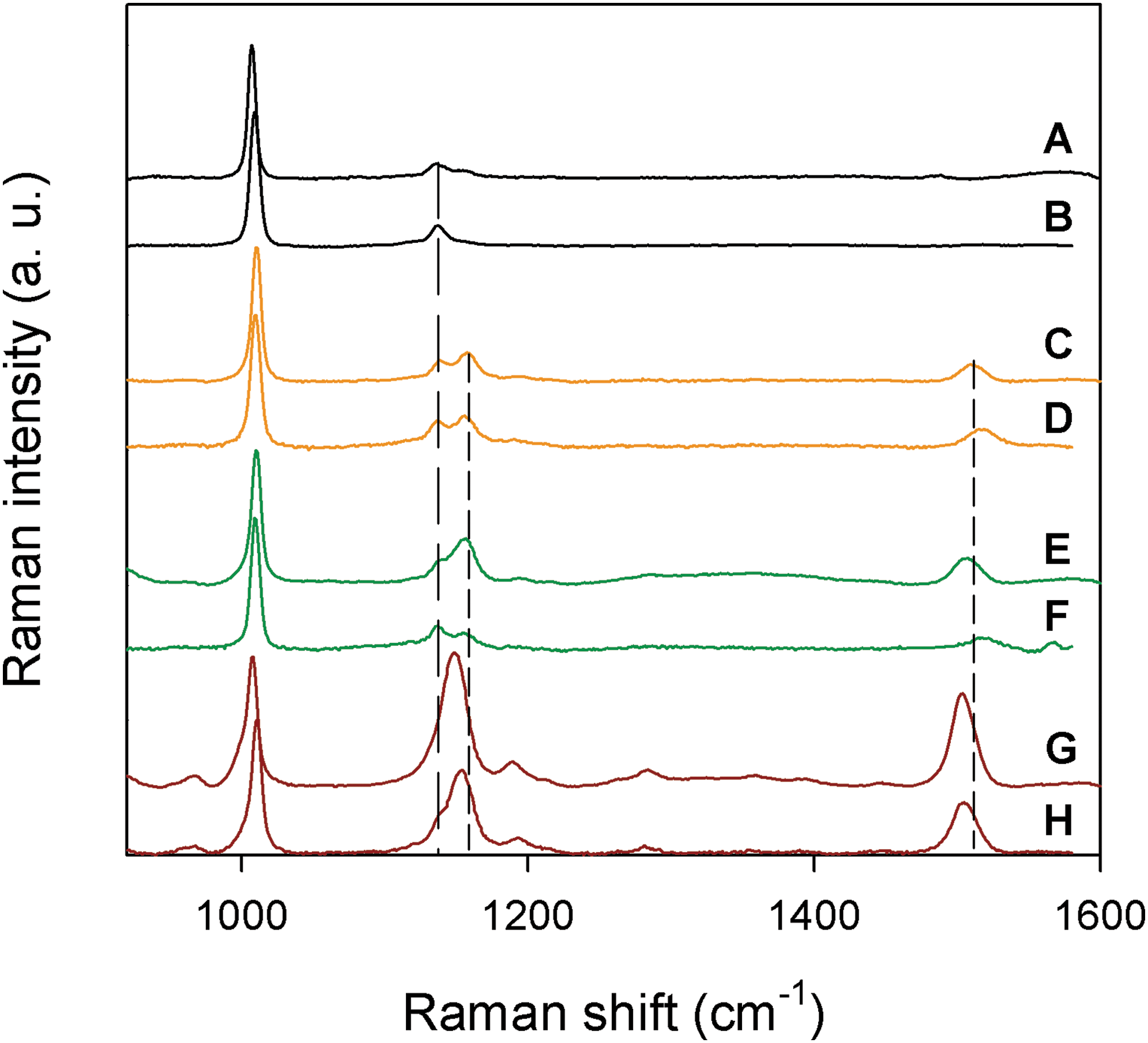
Representative Raman spectra obtained with the Advantage spectrometer (using an excitation wavelength at 532 nm) are presented in Fig. 3. Two distinct types of spectra were observed. The first type was obtained from the first layer of the sulfate crust (i.e., sample C1, Fig. 3A, and sample P1, Fig. 3B). Each spectrum from these samples consisted of two bands that corresponded to gypsum, the dihydrated form of calcium sulfate (CaSO₄·2H₂O). The more intense band (ν₁ at ∼1007 cm⁻¹) originates from the symmetric stretch vibration of the sulfate tetrahedron, while the lower-intensity band (ν₃ at ∼1137 cm⁻¹) originates from the antisymmetric stretch vibration of the sulfate tetrahedron (Wang and Zhou, 2014). The second type of spectrum was obtained from the colored layers, where bands corresponding to the resonant Raman signature of carotenoids (with the three typical bands at about 1005, 1150–1155, and 1510–1520 cm⁻¹) were observed. The orange layer (sample C2, Fig. 3C, and sample P2, Fig. 3D) exhibited the carotenoid resonant Raman bands at 1005, 1154, and 1515 cm⁻¹, while the green layer (sample C3, Fig. 3E, and sample P3, Fig. 3F), exhibited the carotenoid bands at 1005, 1154, and 1516 cm⁻¹ (i.e., no apparent shift in band position was noticed between the orange and green layers). However, in the red layer, the carotenoid bands were detected at 1005, 1151, and 1510 cm⁻¹ (sample C4, Fig. 3G, and sample P4, Fig. 3H). That is, the positions of the last two resonant bands were observed to be shifted to smaller Raman shift values (compared to those obtained from the orange and green layers). This position shift is emphasized in Fig. 3 by the dotted lines. Figure 3 also highlights the fact that the contribution of the sulfate to the spectral intensity was more significant for the powder samples (i.e., the intensity of the band at 1007 cm⁻¹ relative to the intensity of the 1510–1515 cm⁻¹ band was higher for the powder samples). This effect was most apparent for sample P3 (see Fig. 3F), for which the carotenoid band at 1154 cm⁻¹ was seen to include a shoulder at lower Raman shifts. This feature resulted from the lower-intensity gypsum band located at 1137 cm⁻¹ (see Fig. 3).

FIG. 3.

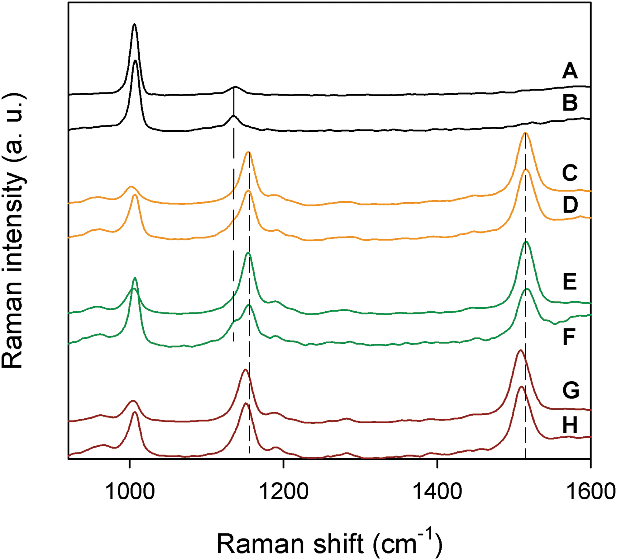
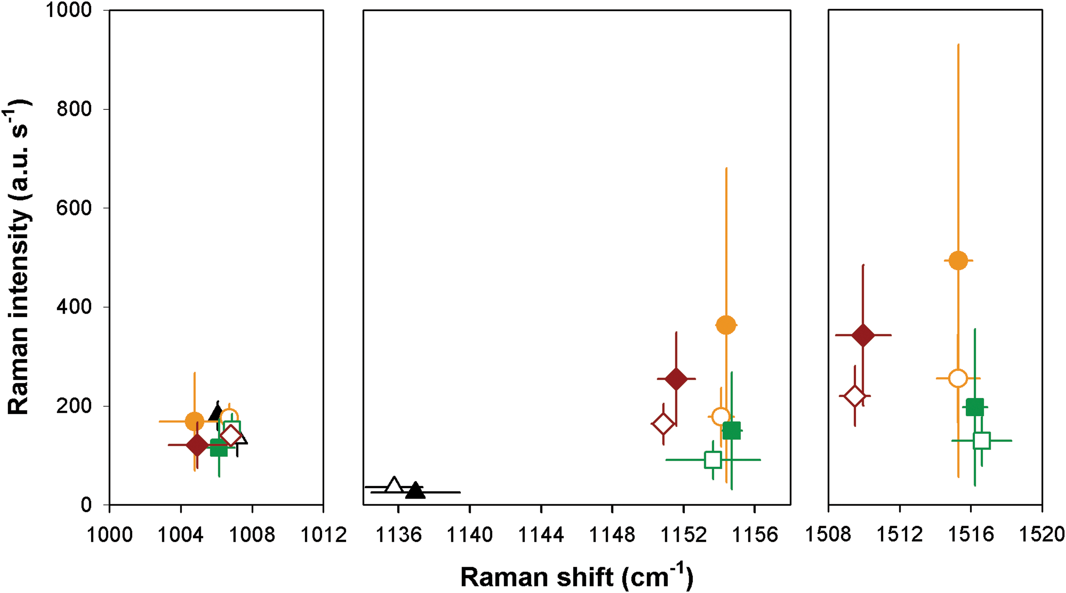
Average of 10 Raman spectra recorded on the different samples of the sulfate crust with an Advantage Raman spectrometer using a 532 nm excitation wavelength. (A) Sample C1, transparent crystal (acquisition time of 20 s); (B) powder sample P1, ground transparent crystals (acquisition time of 10 s); (C) sample C2, orange crystal (acquisition time of 10 s); (D) sample P2, ground orange crystals (recording time of 15 s); (E) sample C3, green crystal (acquisition time of 10 s); (F) sample P3, ground green crystals (acquisition time of 10 s); (G) sample C4, red crystal (acquisition time of 10 s); and (H) sample P4, ground red crystals (acquisition time of 15 s).

The position and intensity of the observed Raman bands are presented in Fig. 4 for crystal samples (C1 to C4, filled symbols) and for powder samples (P1 to P4, unfilled symbols) studied with the commercial portable instrument and the 532 nm excitation wavelength. For each location on the samples (represented by one data point in Fig. 4), the observed fluctuation in band position and band intensity is indicated by the size of the error bars (which represent the standard deviations observed across 10 repeated measurements). With this commercial portable instrument, the resonant Raman signal of carotenoids was observed at ∼1515 cm⁻¹ with a higher intensity compared to the classic Raman signal of gypsum at ∼1008 cm⁻¹, though gypsum was the mineral matrix and was thereby expected to represent a higher fraction of the sample components. This demonstrates once more that carotenoids are an interesting scientific target for planetary exploration when using Raman spectrometers equipped with a green excitation wavelength (such as the 532 nm excitation line on board the ExoMars rover) because they exhibit a resonance effect. The resonance effect increases the chance of detecting organic material (such as carotenoids), especially when it is found in low quantity dispersed in mineralogical matrix (such as gypsum). The classical Raman light scattered by organic molecules is indeed likely to be overwhelmed by the signal of the inorganic compounds [which have a higher scattering cross section (Edwards et al., 2013)].

FIG. 4.

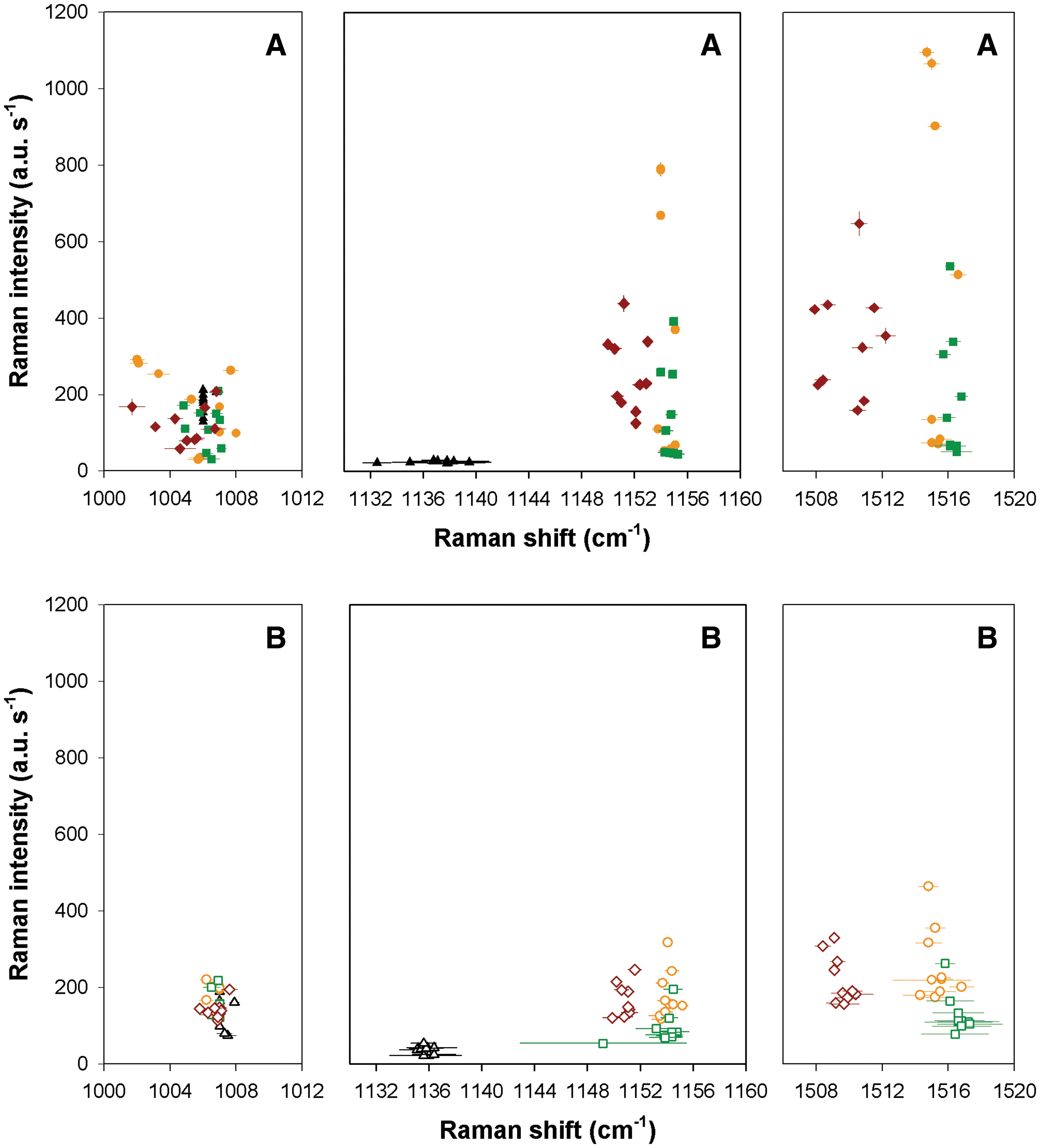
Positions and intensities of the Raman bands observed in the spectra obtained for the crystal samples (black ▲ = C1, orange ● = C2, green ■ = C3, and red ♦ = C4) and for the powder samples (black △ = P1, orange ○ = P2, green □ = P3, and red ◊ = P4) using a commercial instrument and a 532 nm excitation wavelength. Each point represents the average position and the average intensity obtained from one given location on the sample (calculated from 10 replicate spectra). The error bars represent the standard deviations calculated based on the 10 replicate spectra.

3.2. Data obtained with the RLS prototype instrument (532 nm)

An identical description stood for the spectra obtained with an ExoMars RLS prototype when using an excitation wavelength at 532 nm (representative spectra are presented in Fig. 5). However, the sensitivity of the instrument for carotenoid signals was lower compared to the sensitivity of the commercial portable spectrometer (see Fig. 3). This difference in sensitivity can be related to the difference in design of the two instruments compared in this paper. Indeed, the excitation laser beam was focused on the sample by a lens with the commercial portable spectrometer, while it was focused by a microscope objective with the ExoMars RLS prototype. Consequently, the laser spot on the sample surface was larger with the commercial spectrometer than it was with the prototype; therefore, more carotenoid material was sampled. Another fundamental experimental difference was the collection of the Raman light that was collected backward and directly sent to the grating (wavelength separator) with the commercial instrument but passed through an optical fiber in the prototype (Hutchinson et al., 2014). Due to its restricted section, the optical fiber acts as a confocal pinhole decreasing the volume actually sampled in depth in the sample (and so the amount of carotenoids observed). The ν₃ band of gypsum (at ∼1137 cm⁻¹) and the ν₂ band of carotenoids (∼1155 cm⁻¹) were more resolved than they were with the commercial instrument. This is a direct consequence of the higher spectral resolution achieved with the prototype (∼3 cm⁻¹) compared to the one characterizing the commercial instrument (∼10 cm⁻¹).

FIG. 5.

Average of 10 Raman spectra recorded on the different samples of the sulfate crust with an ExoMars RLS prototype that is being developed at the University of Leicester using a 532 nm excitation wavelength. (A) Sample C1, transparent crystal (acquisition time of 6 s); (B) powder sample P1, ground transparent crystals (acquisition time of 7 s); (C) sample C2, orange crystal (acquisition time of 9 s); (D) sample P2, ground orange crystals (recording time of 6 s); (E) sample C3, green crystal (acquisition time of 7 s); (F) sample P3, ground green crystals (acquisition time of 14 s); (G) sample C4, red crystal (acquisition time of 12 s); and (H) sample P4, ground red crystals (acquisition time of 14 s).

3.3. Relative intensities of gypsum and carotenoids using a 532 nm laser

For spectra acquired at different locations on the crystal samples (represented by different dots in Fig. 4), the absolute intensities fluctuated to a great extent. This fluctuation was not due to any temporal variation in the amount of scattered light received by the detector. Indeed, the reproducibility of the Raman intensity at one given location on the sample (represented by error bars in Fig. 4) is lower than the variation of the intensity between locations.

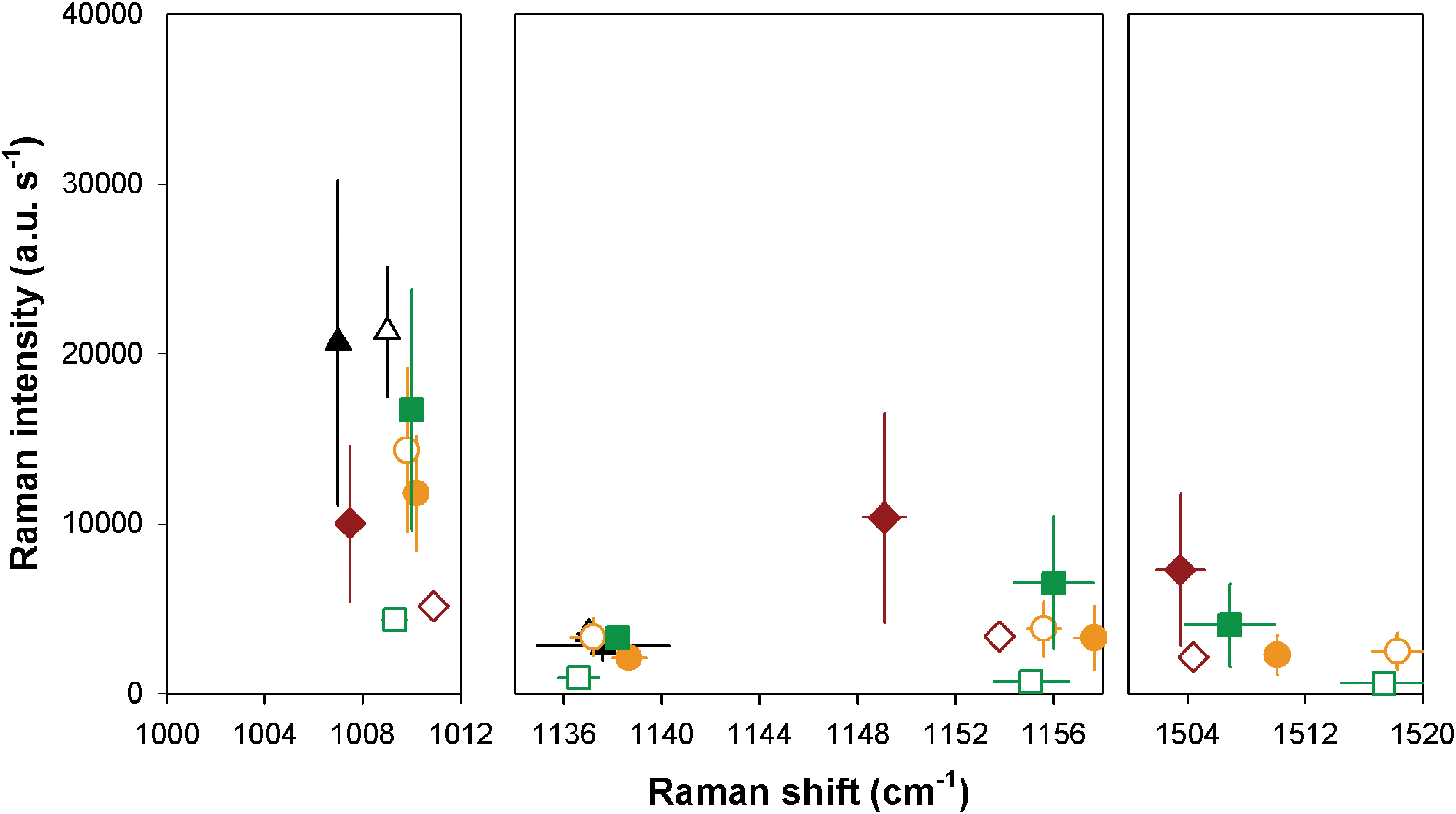
In Figs. 6 and 7, graphical summaries of the intensities and band positions obtained for each sample (average results obtained for 10 locations on each sample) are provided. Although the fluctuation of intensity (represented by the error bars in Figs. 6 and 7) is still observed for the powder samples, it was found to be of less significance. Indeed, the standard deviations were found to be reduced for the powder samples. Also, the intensity of the carotenoid bands in powder samples was reduced (to about half the intensity measured on crystal samples). This observation indicates that the carotenoids are more distributed in the powder samples than in the crystal samples. It also means that Raman data acquired from powder samples are more representative of the entire sample than data acquired from the original crystal samples.

FIG. 6.

Positions and intensities of the Raman bands observed in the spectra obtained for the crystal samples (black ▲ = C1, orange ● = C2, green ■ = C3, and red ♦ = C4) and for the powder samples (black △ = P1, orange ○ = P2, green □ = P3, and red ◊ = P4) using a commercial instrument and a 532 nm excitation wavelength. Each point represents the average position and the average intensity obtained from all spectra for a given sample (calculated from typically 100 spectra). The error bars represent the standard deviations calculated based on the 10 replicate spectra.

FIG. 7.

Positions and intensities of the Raman bands observed in the spectra obtained for the crystal samples (black ▲ = C1, orange ● = C2, green ■ = C3, and red ♦ = C4) and for the powder samples (black △ = P1, orange ○ = P2, green □ = P3, and red ◊ = P4) using an ExoMars RLS prototype instrument and a 532 nm excitation wavelength. Each point represents the average position and the average intensity obtained from all spectra for a given sample (calculated from typically 10 spectra). The error bars represent the standard deviations calculated based on the 10 replicate spectra.

3.4. Position of the Raman bands of gypsum and carotenoids using a 532 nm laser

Table 1 summarizes the band positions observed when an excitation wavelength at 532 nm was used to generate the Raman spectra with the commercial portable spectrometer or the ExoMars RLS prototype. Several observations are apparent from that table.

Table 1.

Band Positions and Intensities Obtained for Eight Samples of the Sulfate Crust Recovered from Eilat Salterns

	Band ν₃(C-CH₃)/ν₁(SO₄ ²⁻)						Band ν₃(SO₄ ²⁻)						Band ν₂(C-C)						Band ν₁(C═C)
Samples	Position (cm⁻¹) Mean ± SD			Intensity (a.u. s⁻¹) Mean ± SD			Position (cm⁻¹) Mean ± SD			Intensity (a.u. s⁻¹) Mean ± SD			Position (cm⁻¹) Mean ± SD			Intensity (a.u. s⁻¹) Mean ± SD			Position (cm⁻¹) Mean ± SD			Intensity (a.u. s⁻¹) Mean ± SD
532 nm excitation wavelength (Advantage)
C1	1006.1	±	0.3	180	±	30	1137	±	2	25	±	4
C2	1005	±	2	200	±	100							1154.4	±	0.6	400	±	300	1515.3	±	0.8	500	±	400
C3	1006.1	±	0.9	120	±	60							1154.7	±	0.5	100	±	100	1516.2	±	0.7	200	±	200
C4	1005	±	2	120	±	50							1152	±	1	300	±	100	1510	±	2	300	±	100
P1	1007.2	±	0.4	130	±	40	1136	±	2	40	±	10
P2	1006.7	±	0.5	180	±	30							1154.1	±	0.7	180	±	60	1515	±	1	250	±	90
P3	1006.9	±	0.4	150	±	30							1154	±	3	90	±	40	1517	±	2	130	±	50
P4	1006.8	±	0.6	140	±	20							1150.9	±	0.7	160	±	40	1509.5	±	0.9	220	±	60

532 nm excitation wavelength (ESA prototype)
C1	1007.0	±	no SD	20000	±	10000	1138	±	3	2800	±	900
C2	1010.2	±	0.4	12000	±	3000	1138.7	±	0.7	2100	±	500	1157.7	±	0.9	3000	±	2000	1510.1	±	0.8	2000	±	1000
C3	1010.0	±	no SD	17000	±	7000	1138.2	±	0.4	3200	±	500	1156	±	2	7000	±	4000	1507	±	3	4000	±	2000
C4	1007.5	±	0.5	10000	±	5000							1149.1	±	0.9	10000	±	6000	1504	±	2	7000	±	4000
P1	1009.0	±	no SD	21000	±	4000	1137.0	±	0.5	3531	±	600
P2	1009.8	±	0.4	14000	±	5000	1137.2	±	0.9	3326	±	1100	1155.6	±	0.7	4000	±	2000	1518	±	2	2000	±	1000
P3	1009.3	±	0.5	4300	±	300	1136.6	±	0.8	936	±	80	1155	±	2	710	±	80	1517	±	3	600	±	60
P4	1010.9	±	0.3	5200	±	700							1153.8	±	0.4	3400	±	400	1504.4	±	0.5	2100	±	200

785 nm excitation wavelength (Raman Inspector)
C1	1008.2	±	0.9	1700	±	900	1132	±	8	190	±	90
C2	1008.4	±	0.7	2000	±	1000	1139	±	2	190	±	90
C3	1008.6	±	0.6	1700	±	600	1134	±	7	310	±	50
C4
P1	1007.5	±	0.7	340	±	90	1135.8	±	1.1	80	±	20
P2	1009.6	±	0.5	800	±	200	1137.5	±	1.5	210	±	50
P3	1009.9	±	0.8	900	±	300	1137.9	±	1.4	210	±	70
P4

The results were calculated based on a set of 100 spectra (10 replicates obtained at 10 different locations). C = crystal samples, P = powder samples, 1 = recovered from the transparent layer, 2 = recovered from the yellow-orange layer, 3 = recovered from the green layer, 4 = recovered from the red layer, and SD = standard deviation.

Firstly, two Raman bands were detected between 1000 and 1010 cm⁻¹, one belonging to gypsum (expected at ∼1007 cm⁻¹), while the other belongs to carotenoids (expected at ∼1005 cm⁻¹). These bands were too close to each other to be resolved with flight representative spectrometers; therefore, only one band appeared to be detected between 1005 and 1007 cm⁻¹ with the Advantage spectrometer and between 1007 and 1011 cm⁻¹ with the RLS prototype. The standard deviation (SD) of the band position indicated that the position of this band is more repeatable for powder samples compared to the crystal samples. This observation was again linked to the homogeneity of the powder samples by opposition to the crystal samples. The improved dispersion of the carotenoid molecule in the powder samples led to similar spectra (in terms of carotenoid/gypsum intensity ratios). Consequently, the reproducibility of the observed spectra was increased for the powder samples. For the samples C1 and P1, only the signal of gypsum was detected at 1006.1 ± 0.3 cm⁻¹ and at 1007.2 ± 0.4 cm⁻¹ (for C1 and P1, respectively) with the Advantage spectrometer and at 1007.0 cm⁻¹ and at 1009 cm⁻¹ (for C1 and P1, respectively) with the RLS prototype (the standard deviation was not calculated, since the band position was found to be identical for all 10 spectra).

Secondly, two bands were found between 1130 and 1160 cm⁻¹, which are not entirely resolved: the ν₃ band of gypsum observed at ∼1137 cm⁻¹ with both spectrometers (RLS prototype and Advantage) and the ν₂ band of carotenoids located between 1151 and 1156 cm⁻¹ depending on the colored layer analyzed. When using the RLS prototype, the ν₃ band of gypsum and the ν₂ band of carotenoids were better resolved and of similar intensity; then two maxima were distinctly observed, and their positions are reported in Table 1. The position of the ν₃ band of gypsum was repeatable for all samples. On the contrary, a shift in band position was observed for the ν₂ band of carotenoids between the orange/green layers and the red layer. The shift in position was found to be statistically significant according to a two-tailed t test of the difference of the means at the confidence level of 95%, in most of the cases. For example, the band was located at 1155.6 ± 0.7 cm⁻¹ in the spectra obtained for powder sample from the orange layer and at 1153.8 ± 0.4 cm⁻¹ in the spectra obtained for powder samples from the red layer (both with the ESA prototype). The values should be considered as statistically different since the t value associated with them (7.06) was calculated to be higher than the critical value t _c (2.1, at the confidence level of 0.95 and at a degree of freedom of 14).

Thirdly, the ν₁ band of the carotenoids, which is observed between 1504 and 1517 cm⁻¹, was also found to be shifted in position for the red layer, compared to the orange and green layers. The shift in position of 5–6 cm⁻¹ was systematically observed and was again statistically significant (according to a two-sided t test of the difference of the means at the confidence level of 95%). The shift was observed with both instruments (Advantage and RLS prototype) as shown in Figs. 4, 6, and 7 in which a straight vertical line can generally be drawn to separate the data points from the orange and green layers and those from the red layer. It was confirmed that this shift did not originate from the calibration process. Indeed, the error on the band position between several calibration procedures was never higher than 0.8 cm⁻¹, which is significantly lower than the value of the shift observed.

3.5. Data obtained with the DeltaNu instrument (785 nm)

When the 785 nm excitation wavelength was used to obtain the spectra (a selection is shown in Fig. 8), only the contribution from gypsum was detected. The spectra obtained for samples C1 to C3 (crystal samples of the three first layers) and P1 to P3 (powder samples of the three first layers) were found to be similar to the spectra A and B presented in Fig. 3 (data not shown). In addition, for samples C2, C3, P2, and P3, the Raman signal is observed on a broad band centered at 1400 cm⁻¹ (880 nm in the wavelength scale), which was attributed to the fluorescence of bacteriochlorophyll a. No Raman spectrum was obtained for any of the samples prepared from the red layer (samples C4 and P4). For these samples, the fluorescence signal saturated the detector in less than one second, even when the laser power level of the 785 nm excitation source was set to its lowest level. Fluorescence levels have been used to monitor the vertical distribution of bacteriochlorophyll a at ocean surface (Kolber, 2001), and bacteriochlorophyll a was reported to be present in all layers colonized by microorganisms in the Eilat gypsum crust (Oren et al., 2009). The band positions and intensities of gypsum observed with a 785 nm excitation wavelength are reported in Table 1.

FIG. 8.

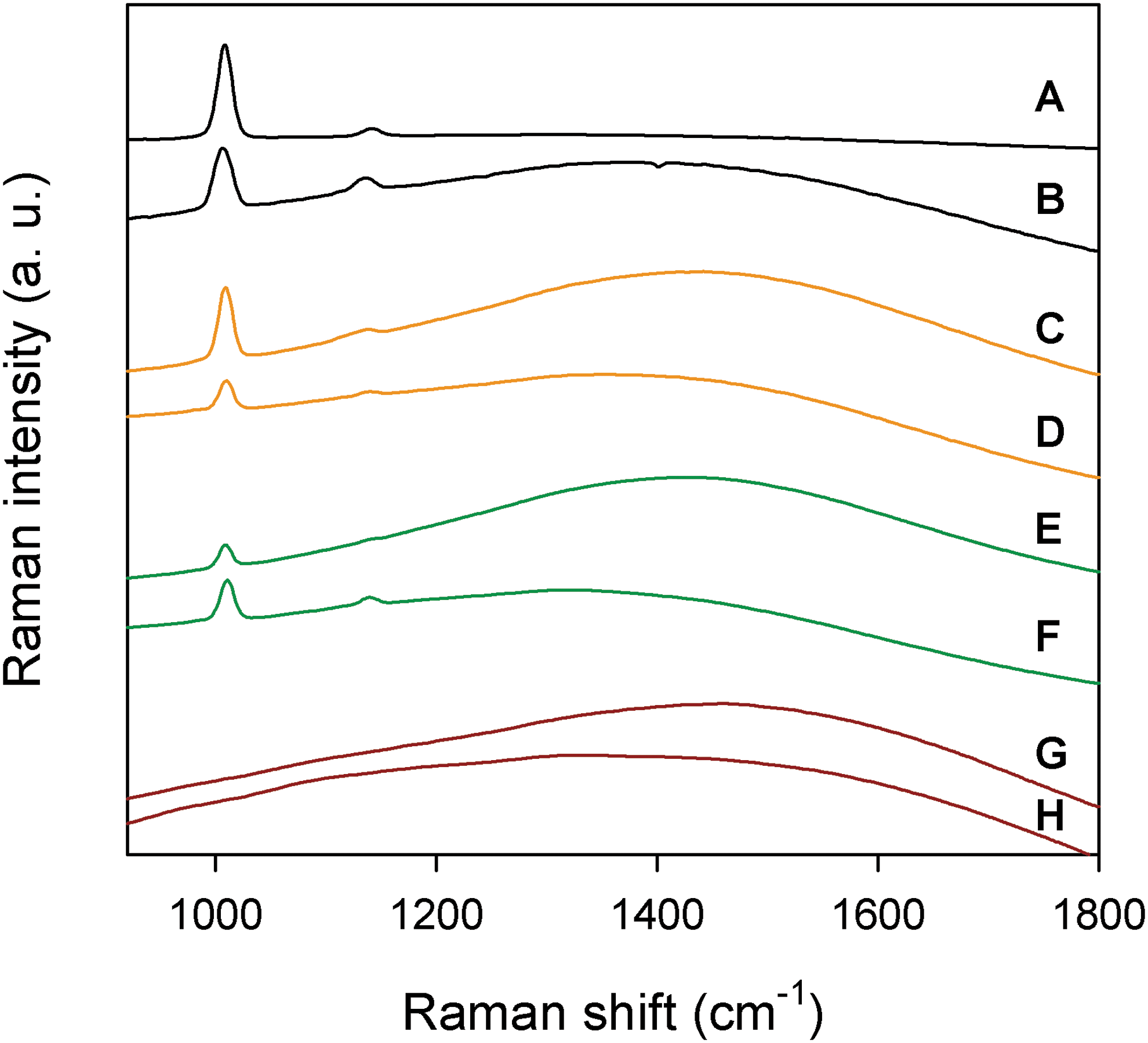
Average of 10 Raman spectra recorded on the different samples of the sulfate crust with a Raman Inspector spectrometer using a 785 nm excitation wavelength. (A) Sample C1, transparent crystal (acquisition time of 10 s); (B) powder sample P1, ground transparent crystals (acquisition time of 20 s); (C) sample C2, orange crystal (acquisition time of 15 s); (D) sample P2, ground orange crystals (recording time of 5 s); (E) sample C3, green crystal (acquisition time of 2 s); (F) sample P3, ground green crystals (acquisition time of 10 s); (G) sample C4, red crystal (acquisition time of 0.1 s); and (H) sample P4, ground red crystals (acquisition time of 0.2 s).

4. Discussion

In a previous study of the Eilat benthic crust in which benchtop, portable, and flight prototype Raman instruments were used, it was concluded that the shift in position was detectable with every instrument except the ESA prototype (Culka et al., 2014). However, the study only included spectral data obtained directly from the crystal samples themselves and is therefore not strictly representative of the ExoMars Sample Preparation and Distribution System (SPDS). Indeed, in the course of the ExoMars mission, martian regolith samples will be crushed and deposited into a well; then the surface will be smoothed with a blade (Hutchinson et al., 2014). Here, we have reported a more systematic study where, for each instrument, one set of data was acquired directly for crystal samples and another was acquired for powder samples (similar to the ExoMars sample preparation strategy). The data acquisitions were straightforward, requiring minimal optimization, and a systematic approach was applied for determining the position of the Raman bands.

The intensity of the carotenoid bands in powder samples was reduced to half the intensity measured for crystal samples, with a smaller variability of the detected intensities (lower standard deviation as shown in Figs. 6 and 7). This observation indicates a higher distribution of the carotenoids in the powder samples, which was expected after the crushing of the crystal samples where local concentrated volumes were interrogated by the Raman spectrometer. A direct implication of the higher biomarker distribution within the powder samples is that the probability of sampling it within the volume analyzed by the spectrometer is increased. This supports the sample preparation approach adopted for the forthcoming ExoMars mission where martian samples will be crushed before analysis by different analytical techniques (Baglioni et al., 2006; ExoMars mission, 2015), which will improve the presence probability of the analyte (biomarker) in the interrogated sample. However, the intensity of the signal can be lessened because the homogeneous overall concentration will be lower than heterogeneous local concentration. There is a risk that the carotenoid concentration level will be below the sensitivity limit of the instrument. The intricate relationship between the homogeneity of the dispersion of a biomarker in solid matrices, the limit of identification, and the limit of detection was previously discussed in the work of Vandenabeele et al. (2012), but this still needs to be experimentally assessed.

Using a 532 nm excitation wavelength, we obtained the results reported in Table 1, which demonstrate that flight representative spectrometers (commercial portable or RLS prototype) are able to detect a shift in ν₁ and ν₂ band positions as low as 3 cm⁻¹ (even if the spectral resolutions of each spectrometer were lower than or equal to that shift). The shift was found to be statistically significant and was not an artifact originating from the calibration process. Actually, the shift of these bands was related to the nature of the carotenoid molecules present in the different layers. Indeed, carotenoids are known to exhibit a resonance Raman scattering when a green excitation line is used (Edwards et al., 2014). The phenomenon originates from a coupling of the excitation photons and the electrons delocalized along the conjugated carbon chain (Ferraro et al., 2003; Smith and Dent, 2004). Since the length of the chain influences the polarizability (the readiness for the electronic cloud around the chromophore to be disturbed), the resonant signal depends also on the chain size. The band intensity will certainly be affected because longer chains will absorb light of lower energy (higher wavelength) (Merlin, 1985; Withnall et al., 2003; Marshall et al., 2007). Most importantly, however, the band position (expressed as Raman shift in cm⁻¹) will decrease with the effective carbon-carbon bond length. When the conjugated chain size increases, the effective bond length decreases and so do the positions of the ν₁ and ν₂ bands. Accordingly, the carotenoid molecule observed in the red layer should have had a longer conjugated carbon chain compared to the carotenoid found in the orange and red layers because the position of the ν₁ and ν₂ bands was found to be lower in the red layer (as can been seen in Table 1). This is consistent with other studies performed on similar samples from the Eilat salterns (Jehlička and Oren, 2013b; Jehlička et al., 2014b; Harris et al., 2015), where it was reported that the main carotenoid molecule contained in the red layer is spirilloxanthin (with a 26-carbon conjugated chain), and ν₁ and ν₂ bands were observed at 1151 and 1510 cm⁻¹. The main carotenoid molecules reported to be present in the yellow-orange and green layers were myxoxanthophyll, echinenone, and β-carotene (with a 24-, 22-, and 22-carbon conjugated chain, respectively), and ν₁ and ν₂ bands were observed at 1155 and 1515–1516 cm⁻¹. No statistical difference in position was observed for ν₁ and ν₂ bands between the yellow-orange layer and the green layer. It must also be noted that, while a significant shift in band position was observed between the red layer and the orange and green layers of the benthic gypsum crust, the association of the resonant signal with a specific carotenoid is not feasible based only on Raman data. Indeed, the interaction of carotenoid molecules with the hosting inorganic environment and the possible aggregation of several carotenoid molecules can also influence the band position (de Oliveira et al., 2010). Nevertheless, we demonstrate here that, should the mineral host be identical for different samples (which is the case here for the different layers), the prototype Raman instrument can detect a change in the length of the polyene backbone of the resonant carotenoids.

Finally, when using a 785 nm excitation wavelength, no Raman signal from organic molecules was discerned from the fluorescence background, contrary to previous expectations (Culka et al., 2014). Actually, the fluorescence due to bacteriochlorophyll a is seen to overwhelm any Raman signature generated by organic compounds. Only the signature of gypsum was detected and only for the three first layers (transparent, yellow-orange, and green layers), where the quantity of bacteriochlorophyll a was reported to be lower than in the fourth one (red layer) (Oren et al., 2009).

5. Conclusion

The four outer layers observed in a benthic gypsum crust of saltern ponds in Eilat, Israel, were analyzed with flight representative Raman spectrometers, two commercial portable spectrometers and the RLS prototype developed at the University of Leicester. Two excitation wavelengths were used (532 and 785 nm). The gypsum nature of the crust is readily identified based on the Raman signature detected by the three spectrometers, with both excitation wavelengths. Using a 532 nm laser source, we were able to detect carotenoids due to their resonant Raman signal, simultaneously with gypsum. We observed a significant downward shift as large as 5–6 cm⁻¹ in position for dispersive bands of carotenoids (ν₂ at ∼1150 cm⁻¹ and ν₁ at ∼1550 cm⁻¹) when considering the red layer compared to the upper green and orange layers. We demonstrated that different members of the carotenoid family can be detected with miniaturized Raman spectrometers. We also demonstrated that the RLS prototype developed at the University of Leicester is characterized by a higher resolution than the commercial analogues since the ν₃ band of gypsum (at ∼1137 cm⁻¹) and the ν₂ band of carotenoid (at ∼1155 cm⁻¹) were partially resolved with the prototype instrument but not with the commercial instruments.

Footnotes

Acknowledgments

C.M., H.G.M.E., I.B.H. and R.I. acknowledge the support of the STFC Research Council and the UK Space Agency in the UK ExoMars programme, and M.M. acknowledges studentship support from the European Space Agency through the Network/Partnership scheme. We thank Salt of the Earth Eilat Ltd. for allowing access to the salterns, and the Interuniversity Institute of Marine Sciences of Eilat for logistic support.

Author Disclosure Statement

No competing financial interests exist.

Abbreviation Used

References

Baglioni

, Fisackerly

, Gardini

, Gianfiglio

, Pradier

A.L.

, Santovincenzo

, Vago

J.L.

, and Van Winnendael

(2006) The Mars exploration plans of ESA. IEEE Robot Autom Mag, 13:83–89.

Culka

, Osterrothova

, Hutchinson

, Ingley

, McHugh

, Oren

, Edwards

H.G.M.

, and Jehlička

(2014) Detection of pigments of halophilic endoliths from gypsum: Raman portable instrument and European Space Agency's prototype analysis. Philos Transact A Math Phys Eng Sci, 372, doi:10.1098/rsta.2014.0203.

de Oliveira

V.E.

, Castro

H.V.

, Edwards

H.G.M.

, and de Oliveira

L.F.C.

(2010) Carotenes and carotenoids in natural biological samples: a Raman spectroscopic analysis. J Raman Spectrosc, 41:642–650.

Edwards

H.G.M.

, Hutchinson

I.B.

, Ingley

, Parnell

, Vítek

, and Jehlička

(2013) Raman spectroscopic analysis of geological and biogeological specimens of relevance to the ExoMars mission. Astrobiology, 13:543–549.

Edwards

H.G.M.

, Hutchinson

I.B.

, Ingley

, and Jehlička

(2014) Biomarkers and their Raman spectroscopic signatures: a spectral challenge for analytical astrobiology. Philos Transact A Math Phys Eng Sci, 372, doi:10.1098/rsta.2014.0193.

ExoMars mission. (2015) ExoMars mission. 2018. European Space Agency, Paris. Available online at http://exploration.esa.int/mars/48088-mission-overview

Ferraro

J.R.

, Nakamoto

, and Brown

C.W.

(2003) Introductory Raman Spectroscopy, 2 ^nd ed., edited by Ferraro

J.R.

, Nakamoto

, and Brown

C.W.

, Academic Press, San Diego.

Gendrin

, Mangold

, Bibring

J.-P.

, Langevin

, Gondet

, Poulet

, Bonello

, Quantin

, Mustard

, Arvidson

, and LeMouélic

(2005) Sulfates in martian layered terrains: the OMEGA/Mars Express view. Science, 307:1587–1591.

Grotzinger

J.P.

, Sumner

D.Y.

, Kah

L.C.

, Stack

, Gupta

, Edgar

, Rubin

, Lewis

, Schieber

, Mangold

, Milliken

, Conrad

P.G.

, Des Marais

, Farmer

, Siebach

, Calef

III , Hurowitz

, McLennan

S.M.

, Ming

, Vaniman

, Crisp

, Vasavada

, Edgett

K.S.

, Malin

, Blake

, Gellert

, Mahaffy

, Wiens

R.C.

, Maurice

, Grant

J.A.

, Wilson

, Anderson

R.C.

, Beegle

, Arvidson

, Hallet

, Sletten

R.S.

, Rice

, Bell

III , Griffes

, Ehlmann

, Anderson

R.B.

, Bristow

T.F.

, Dietrich

W.E.

, Dromart

, Eigenbrode

, Fraeman

, Hardgrove

, Herkenhoff

, Jandura

, Kocurek

, Lee

, Leshin

L.A.

, Leveille

, Limonadi

, Maki

, McCloskey

, Meyer

, Minitti

, Newsom

, Oehler

, Okon

, Palucis

, Parker

, Rowland

, Schmidt

, Squyres

, Steele

, Stolper

, Summons

, Treiman

, Williams

, Yingst

; MSL Science Team. (2014) A habitable fluvio-lacustrine environment at Yellowknife Bay, Gale Crater, Mars. Science, 343, doi:10.1126/science.1242777.

10.

Harris

L.V.

, McHugh

, Hutchinson

I.B.

, Ingley

, Malherbe

, Parnell

, Olcott Marshall

, and Edwards

H.G.M.

(2015) Avoiding misidentification of bands in planetary Raman spectra. J Raman Spectrosc, 46:863–872.

11.

Hutchinson

I.B.

, Ingley

, Edwards

H.G.M.

, Harris

, McHugh

, Malherbe

, and Parnell

(2014) Raman spectroscopy on Mars: identification of geological and bio-geological signatures in martian analogues using miniaturized Raman spectrometers. Philos Transact A Math Phys Eng Sci, 372, doi:10.1098/rsta.2014.0204.

12.

Jehlička

and Oren

(2013a) Raman spectroscopy in halophile research. Front Microbiol, 4, doi:10.3389/fmicb.2013.00380.

13.

Jehlička

and Oren

(2013b) Use of a handheld Raman spectrometer for fast screening of microbial pigments in cultures of halophilic microorganisms and in microbial communities in hypersaline environments in nature. J Raman Spectrosc, 43:1275–1280.

14.

Jehlička

, Edwards

H.G.M.

, and Oren

(2014a) Raman spectroscopy of microbial pigments. Appl Environ Microbiol, 80:3286–3295.

15.

Jehlička

, Edwards

H.G.M.

, Osterrothova

, Novotna

, Nedbalova

, Kopecky

, Nemec

, and Oren

(2014b) Potential and limits of Raman spectroscopy for carotenoid detection in microorganisms: implications for astrobiology. Philos Transact A Math Phys Eng Sci, 372, doi:10.1098/rsta.2014.0199.

16.

Jorge Villar

S.E.

and Edwards

H.G.M.

(2006) Raman spectroscopy in astrobiology. Anal Bioanal Chem, 384:100–113.

17.

Kolber

Z.S.

(2001) Contribution of aerobic photoheterotrophic bacteria to the carbon cycle in the ocean. Science, 292:2492–2495.

18.

Lopez-Reyes

, Rull

, Venegas

, Westall

, Foucher

, Bost

, Sanz

, Catalá-Espí

, Vegas

, Hermosilla

, Sansano

, and Medina

(2013) Analysis of the scientific capabilities of the ExoMars Raman laser spectrometer instrument. European Journal of Mineralogy, 25:721–733.

19.

Marshall

C.P.

, Leuko

, Coyle

C.M.

, Walter

M.R.

, Burns

B.P.

, and Neilan

B.A.

(2007) Carotenoid analysis of halophilic archaea by resonance Raman spectroscopy. Astrobiology, 7:631–643.

20.

McCreery

R.L.

(2001) Raman spectroscopy for chemical analysis. Meas Sci Technol, 12:653–654.

21.

Merlin

J.C.

(1985) Resonance Raman spectroscopy of carotenoids and carotenoid-containing systems. Pure Appl Chem, 57:785–792.

22.

Moynihan

H.A.

and O'Hare

I.P.

(2002) Spectroscopic characterisation of the monoclinic and orthorhombic forms of paracetamol. Int J Pharm, 247:179–185.

23.

NASA Mars 2020. (2014) NASA announces Mars 2020 rover payload to explore the Red Planet as never before. NASA's Mars Exploration Program, Washington, DC. Available online at http://nasa.gov/press/2014/july/nasa-announces-mars-2020-rover-payload-to-explore-the-red-planet-as-never-before

24.

Oren

(2014) Halophilic archaea on Earth and in space: growth and survival under extreme conditions. Philos Transact A Math Phys Eng Sci, 372, doi:10.1098/rsta.2014.0194.

25.

Oren

and Rodriguez-Valera

(2001) The contribution of halophilic bacteria to the red coloration of saltern crystallizer ponds. FEMS Microbiol Ecol, 36:123–130.

26.

Oren

, Sørensen

K.B.

, Canfield

D.E.

, Teske

A.P.

, Ionescu

, Lipski

, and Altendorf

(2009) Microbial communities and processes within a hypersaline gypsum crust in a saltern evaporation pond (Eilat, Israel). Hydrobiologia, 626:15–26.

27.

Rull

, Sansano

, Díaz

, Canora

C.P.

, Moral

A.G.

, Tato

, Colombo

, Belenguer

, Fernández

, Manfredi

J.A.R.

, Canchal

, Dávila

, Jiménez

, Gallego

, Ibarmia

, Prieto

J.A.R.

, Santiago

, Pla

, Ramos

, Díaz

, and González

(2011) ExoMars Raman laser spectrometer for ExoMars. Proc SPIE, 8152, doi:10.1117/12.896787.

28.

Smith

and Dent

(2004) Modern Raman Spectroscopy: A Practical Approach, John Wiley & Sons, Chichester, UK.

29.

Telfer

(2005) Too much light? How [small beta]-carotene protects the photosystem II reaction centre. Photochem Photobiol Sci, 4:950–956.

30.

Vandenabeele

, Jehlička

, Vítek

, and Edwards

H.G.M.

(2012) On the definition of Raman spectroscopic detection limits for the analysis of biomarkers in solid matrices. Planet Space Sci, 62:48–54.

31.

Wang

and Zhou

(2014) Experimental comparison of the pathways and rates of the dehydration of Al-, Fe-, Mg- and Ca-sulfates under Mars relevant conditions. Icarus, 234:162–173.

32.

Withnall

, Chowdhry

B.Z.

, Silver

, Edwards

H.G.M.

, and De Oliveira

L.F.C.

(2003) Raman spectra of carotenoids in natural products. Spectrochim Acta A Mol Biomol Spectrosc, 59:2207–2212.