Searching for Atmospheric Bioindicators in Planets around the Two Nearby Stars,Proxima Centauri and Epsilon Eridani—Test Cases for Retrieval of Atmospheric Gases with Infrared Spectroscopy

Abstract

We tested the ability of thermal infrared spectroscopy to retrieve assumed atmospheric compositions for different types of planets orbiting Proxima Centauri and Epsilon Eridani. Six cases are considered, covering a range of atmospheric compositions and some diversity in the bulk composition (rocky, water ocean, hydrogen rich) and the spectral type of the parent star (M and K stars). For some cases, we applied coupled climate chemistry, or climate-only calculations; for other cases, we assumed the atmospheric composition, ground temperature, and surface reflectivity. The IR emission was then calculated from line-by-line radiative transfer models and used to investigate retrieval of input atmospheric species. For the six cases considered, no false positive of the triple bioindicator (H₂O, CO₂, and O₂, in specified conditions) was found. In some cases, results show that the simultaneous acquisition of a visible spectrum would be valuable, for example, when CO₂ is very abundant and its 9.4 μm satellite band hides the 9.6 μm O₃ band in the IR. In each case, determining the mass appears mandatory to identify the planet's nature and have an idea of surface conditions, which are necessary when testing for the presence of life.

1. Introduction

In this paper, a main focus is to discuss practical issues when assessing for potential life signals during IR spectral retrieval of exoplanetary atmospheres. We present test cases of putative planets with assumed properties, for example, for their atmospheres. Then we attempt to retrieve these properties using thermal infrared (IR, 3–18 μm) spectroscopy (Rieke, 2009). We investigate factors that affect the signal-to-noise ratio (S/N), factors that influence the choice of spectral resolution, associated effects upon integration times, and methods for constructing the background continuum.

1.1. Two neighboring stars

Performing remote spectroscopy on nearby, cool stars could provide the first chance to discover signs of life outside the Solar System. Proxima Centauri, with a spectral class M6Ve, is our closest stellar neighbor, located 4.3 light-years away, and is one of the most prolifically studied M dwarf stars. It has an effective temperature of 3050 K with a radius and mass of 14% and 12% that of the Sun, respectively. A major recent discovery (Anglada-Escudé et al., 2016) revealed a planet with a minimum mass of 1.3 Earth masses (Proxima Cen b), which orbits at a distance of 0.05 AU, where it receives ∼65% of the net insolation of Earth. Since the planet is unlikely to transit, its atmospheric characterization is expected to focus on direct imaging, reflection, or thermal phase curve variation (Kreidberg and Loeb, 2016). Studies with an atmospheric column model by Meadows et al. (2018a; see also Turbet et al., 2016) suggest habitable conditions if the planet (1) formed further out (hence avoiding likely desiccation during the early stages) and/or (2) possesses a thick, protective H₂ envelope from the protoplanetary disk during its formation. The weak insolation suggests that a strong greenhouse effect would be needed to maintain surface habitability, for example via a surface pressure of several bar of CO₂. Three-dimensional model studies of Proxima Cen b by Kane et al. (2017) support this idea.

Epsilon Eridani is a K2V star with a radius and mass of 84% and 85% that of the Sun, respectively. It is located 10.5 light-years away from us and has at least one gaseous planet (Hatzes et al., 2000). There have been numerous model studies focusing on the potential habitability and biomarkers of hypothetical planets orbiting in the habitable zone (HZ) of Epsilon Eridani (e.g., Segura et al., 2003; Grenfell et al., 2007; Godolt et al., 2016). These works analyzed photochemical and climate effects in the planetary atmosphere related to a redward shift in the incoming stellar spectrum, compared to that of the Sun.

1.2. Assessing potential signals of life

In exoplanet science, the terms “biosignature” and “biomarker” are often used synonymously (see, e.g., Grenfell et al., 2007; Kaltenegger, 2017) and refer to the inability to account for a given signal without invoking the presence of biological activity. An example would be the discovery of an Earth-like planet (on a similar orbit as Earth orbiting a G type star) with an oxygen-rich atmosphere and/or an ozone layer that is similar to those of our home planet. The term “bioindicator” in those works refers to an interesting discovery that could indicate life but requires further information. Given our continuously expanding knowledge of potential abiotic sources, future discoveries of potential life signals are anticipated to trigger discussion that will evolve with our knowledge of the environmental context (stellar insolation, history, planetary bulk, orbital, interior, and atmospheric properties, etc.) as summarized in recent reviews by Grenfell (2017), Schwieterman et al. (2018), and Meadows et al. (2018a,b).

The present paper uses the term bioindicator, defined here as “a set of observable planetary features, such as mass, radius, atmospheric composition, surface temperature, parent star properties, and evolution, etc., that our present models cannot reproduce when including known abiotic photo, -physical, and -chemical processes” (Léger et al., 2011). The latter paper employs the term biosignature for that, but we now prefer to use bioindicator since it is more evocative of a conservative pathway toward the detection of life based upon eliminative iteration via step-by-step scientific debate. This philosophy is supported by the comprehensive review papers in exoplanetary biosignature science stemming from the NASA NExSS workshops; see for instance the work of Kiang et al. (2018), which emphasizes the approach of interpreting potential signals of life within their full environmental and evolutionary context.

In this paper, we also use the terms “false positive” and “false negative.” False positive refers to a set of observations that are falsely interpreted as implying biological activity. Correctly discounting possible false positives is essential when accepting or rejecting a bioindicator. False negatives refer to life not found by our search programs.

All the bioindicators we will likely detect in the near to midterm future will be based on global atmospheric changes driven by life. Detecting such life is facilitated if it perturbs its environment on a planetary scale. Clearly, life located only in small niches is likely to be more difficult to detect remotely, or may not be detected at all (a case of false negative). The case of Mars illustrates the challenge of detecting life remotely. Although Mars has been observed from Earth with an accuracy far superior to that which we can hope for any object outside the Solar System, and sophisticated probes have even been sent to the planet, we still do not know whether life is present on, or under, the martian surface.

2. Model Descriptions

2.1. Atmospheric model

We apply several similar models. All are one-dimensional (1D) cloud-free, coupled radiative-convective-climate-photochemical models. They calculate the steady-state global mean temperature and concentration profiles of (exo)planetary atmospheres. They are described in the works of Rauer et al. (2011), von Paris et al. (2010, 2015), and Tian et al. (2014). For each test case, the model used is specified in Table 1. Models extend from the planetary surface up to P = 6.6 × 10⁻⁵ bar (mid-mesosphere for modern Earth conditions, i.e., ∼65 km; or up to 100 km for the model from Tian et al.). The chemical modules feature over 200 chemical reactions for 55 (or 52 for the model from Tian et al.) long-lived chemical species solved with a backward Euler time-stepping method in 64 model layers (or using a 1 km grid for the model from Tian et al.). Initial abundance and temperature profiles are based on the US standard atmosphere (http://www.pdas.com/atmos.html). Long-lived gases O₂, N₂, and CO₂ are set to constant isoprofile abundances, whereas remaining species are calculated either interactively for the longer-lived species or via the steady-state assumption for short-lived species. In the stratosphere, H₂O is calculated by the chemistry module, whereas in the troposphere it is determined from the temperature profile assuming a relative humidity, RH, profile. It assumes an atmosphere with C_H₂O = RH(z) * P _sat,H₂O(T(z))/P(z), where C_H₂O is the volumetric abundance of H₂O; RH(z), the RH profile; P _sat,H₂O the saturation vapor pressure of H₂O at temperature T(z), and P(z) the atmospheric pressure at height z. RH can be either assumed to be 100% throughout the atmosphere or chosen to be Earth-like, based on Earth observations (Manabe and Wetherald, 1967). Biomass and volcanic and lightning emissions in the chemistry module are based on modern Earth. Dry and wet deposition operate at the lower model boundary, whereas effusion fluxes of CO and O are applied at the upper boundary to simulate the photolysis of CO₂ in the overlying atmosphere.

Table 1.

For the Six Planets Considered: Input Parameters and Models Used for Calculating Their Climate, Chemistry, and IR Emission

Planet type	Case 1 Rocky stripped	Case 2 Water ocean (warm)	Case 3 Rocky CO₂-rich	Case 4 Mini-Neptune	Case 5 Water ocean (hot)	Case 6 Rocky super-Earth
Mpl (Mearth)	4	2	4	4	2	4
Rpl	1.5	1.5	1.5	1.8	1.5	1.5
S		1.0	0.65	1.0	1.05	1.0
a	0.043	0.03	0.049	0.58	0.57	0.58
Star	—————— Proxima Cen (M6V) ——————			——————— eps Eri (K2V) ———————
P_surf (bar)	0	1.21	1	NR	4.58	1
N₂		80%	50%		1 bar	78.36%
O₂		20%	20%		no	19%
CO₂		10⁻⁶	30%		10⁻⁶	10⁻³
H₂O_surf		sat (10 mbar)	sat (10 mbar)		sat (3.58 bar)	Earth-like RH
T_surf (K)	300	280	280	NR	413	292.3
chem calc	no	yes (a)	no	no	no	yes (a)
climate calc	no	yes (b)	no	no	yes (c)	yes (b)
line transfer	no	yes (e)	yes (d)	yes (e)	yes (e)	yes (e)

Model references: (a) Rauer et al., 2011; (b) von Paris et al., 2015; (c) von Paris et al., 2010; (d) Li et al., 2016; (e) García Muñoz et al. (2013).

Mpl = planetary mass; Rpl = planetary radius; S = instellation; a = orbit (AU); NR = not relevant; RH = relative humidity; sat = saturated water pressure.

The climate module employs a two-stream approach (Toon et al., 1989) in the shortwave (237 nm to 4.545 μm) accounting for absorption and scattering by H₂O, CO₂, N₂, O₂, CH₄, O₃, CO, H₂, He. The longwave (1.0–500 μm) scheme features the major atmospheric absorbers (H₂O, CO₂, O₃, and CH₄) using the correlated-k approach (von Paris et al., 2015) for surface temperatures below 400 K calculated from the HITRAN 2012 line database (Rothman et al., 2013). For higher temperatures, the scheme employs the longwave radiative transfer described by von Paris et al. (2010) assuming a simpler atmosphere accounting only for absorption by H₂O, CO₂, and N₂ also using the correlated-k method with absorption coefficients based on the line data of HITEMP 1995 (Rothman et al., 2013). Convective adjustment to the moist adiabatic lapse rate is carried out where applicable.

2.2. Spectral models

We employed two spectral models that are designated (d) and (e) in Table 1. Spectral model (d) is the line-by-line radiative transfer model (LT) described by Li et al. (2016). It uses line intensities and half-widths (both self-broadening and air-broadening) from the HITRAN2012 database (Rothman et al., 2013), with temperature and pressure corrections considered. It calculates the transmission, reflection, and emission spectra of exoplanets. By default, the LT model uses a spectral resolution of 0.01 cm⁻¹ (λ/δλ = 10⁶ and 10⁵ at 1 and 10 μm, respectively). Such a resolution is adequate to resolve all moderately strong lines in the HITRAN2012 database. The high-resolution spectra are reduced to low-resolution spectra by using a triangle smoothing function in order to demonstrate results at λ/δλ = 40 that are used in the paper. Voigt profiles are used for all lines based on the algorithm in Humlíček (1982). A cutoff distance of 50 times the Voigt halfwidth from line centers is applied. Similar to the work of Rein et al. (2014), the effects of clouds and aerosols are ignored in the model. The wavelength-dependent IR spectra for Earth calculated in the LT model are in good agreement with those of Des Marais et al. (2002), hereafter referred to as Des+.

The spectral model (e) in Table 1 uses the output (pressure, temperature, volume mixing ratios) of the 1D radiative-convective-climate-photochemical model to predict the thermal emission from the planet. Ground emissivities and temperatures (see below) are needed to take into account the effect of the surface on the predictions. Synthetic spectra are produced for planet thermal emission with a model that combines the DISORT discrete-ordinate algorithm to solve the radiative transfer problem in the atmosphere (Stamnes et al., 1988) and the 2012 version of the HITRAN database for molecular opacities (Rothman et al., 2013). The model has been extensively used in the investigation of exoplanet and Solar System planet atmospheres (e.g., García Muñoz et al., 2013; García Muñoz and Isaak, 2015; Martins et al., 2018). The synthetic spectra are produced at very high resolving power (λ/δλ ∼ 10⁶) and are subsequently degraded to the resolution of the measurements using a Gaussian profile of the user-input full width at half maximum (FWHM). The model produces a single radiance spectrum that is specific to the planet's center. The irradiance spectrum is finally obtained by scaling the model radiance by the relevant geometrical factors (planetary size and Earth-to-planet distance).

3. Method

This paper investigates potentially habitable planets (both hypothetical and real) with assumed atmospheric compositions, orbiting two nearby stars, namely the M-dwarf Proxima Centauri (M6Ve) and the solar-type star Epsilon Eridani (K2V). Spectral retrieval of atmospheric gases, mainly using thermal IR (3–18 μm) spectroscopy (Rieke, 2009), is subsequently assessed. Several cases address whether the “triple bioindicator” (i.e., the detection of the three gases, H₂O, CO₂, and O₂; based on Selsis et al., 2002) could be achieved under the following specified conditions: (i) the planet is located in the HZ of its star (Kopparapu, 2013), (ii) it has a surface (rocky or liquid)¹, and (iii) P _O₂ ≳ 10 μbar (Harman et al., 2018) and with no indication of a large photolytic water-loss. The constraint on P _O₂ has been recently reduced by 3 orders of magnitude from an older value, 10 mbar (Kasting, 1995; Rosenqvist and Chassefiere, 1995; Tian et al., 2014; Meadows et al., 2018b), by considering the impact of lightning (see Section 5.6). The present paper assumes this lower O₂ threshold. We investigate mainly the IR domain, where O₃ behaves as a proxy for O₂ (see Segura et al., 2003), which is valuable since the former has a strong spectral signature in the IR (9.6 μm fundamental vibration), whereas O₂ has not (Angel et al., 1986).

First, the user fixes the bulk atmospheric composition (N₂, O₂, CO₂); then the atmospheric models calculate the full composition and climate. Based on this, the spectral models calculate theoretical IR emission spectra. This is subsequently used to investigate retrieval capabilities of atmospheric properties for different assumed spectral resolutions and signal-to-noise ratios (adding different levels of noise).

The main goal is to illustrate both the capabilities, as well as the limits, of thermal IR spectroscopy. Atmospheric compositions are chosen arbitrarily, in order to explore the diverse range of uncertainty and aiming to maintain an open mind for the unexpected.

4. Spectral Analysis: How to Determine a Continuum?

Planetary atmospheres considered in this study are assumed to have IR active gases such as H₂O, CO₂, CH₄, O₃, as well as IR inactive ones such as N₂, O₂, and H₂. Although the latter molecules have only weak absorption bands in the thermal IR, they nevertheless feature potentially strong collisional induced absorptions (CIA). As an example, in a telluric planet with 3 bar of N₂, a possible proxy for the Archean Earth, the presence of H₂ with a 10% mixing ratio would produce a substantial change² in the IR spectrum by N₂-H₂ CIA (Wordsworth and Pierrehumbert, 2013). The CIA process is a valuable tool to detect the presence of IR inactive gases.

FIG. 1.

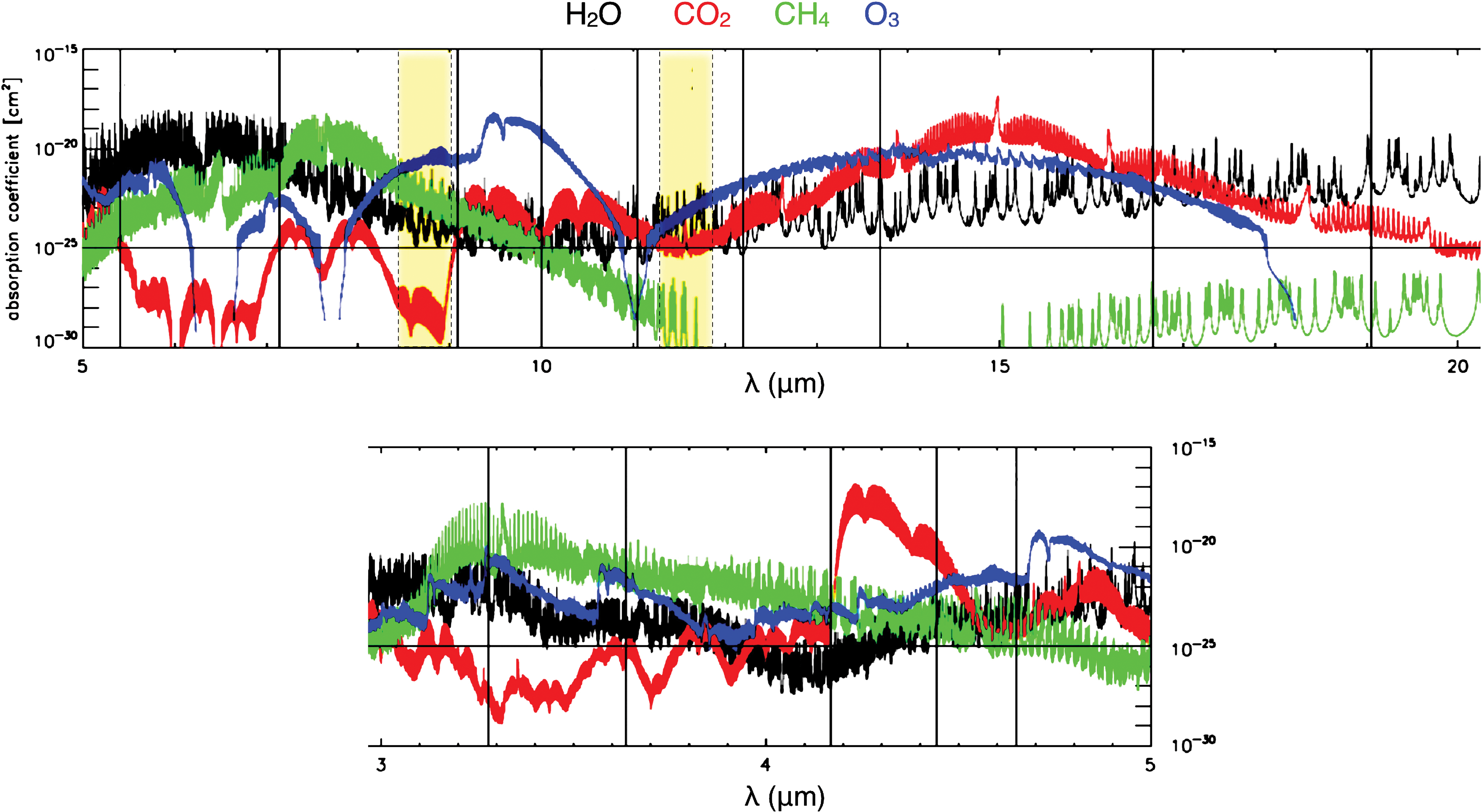
Absorption cross sections of H₂O, CO₂, CH₄, and O₃ gases. Spectroscopic data are from HITRAN 2012 data base Rothman et al. (2013), at T = 300 K and P = 1 bar. Total amplitude of cross section variation is 12 orders of magnitude. Atmospheric windows proposed for Earth-like planets (8.5–9.0 μm, 11.3–11.8 μm) are in light color bands. They correspond to a low absorption for these four gases. Color images available online at www.liebertpub.com/ast

To decide whether these gases can be identified in the spectra, one needs to determine a continuum out of which the bands are detected and measured. This determination should be as objective as possible.

For planets with a possible solid or liquid surface, an atmospheric structure analogous to that of Earth is assumed, that is, an initial decrease of the temperature with altitude as long as the atmosphere is dense and transparent in the visible. Most of the spectral features are then due to gases acting as absorbers. A possible continuum is a Planck function corresponding to the surface temperature. In some cases, the ground can be observed through spectroscopic windows over which the various atmospheric species have small absorption cross sections. The continuum is then fitted to pass through these data points.

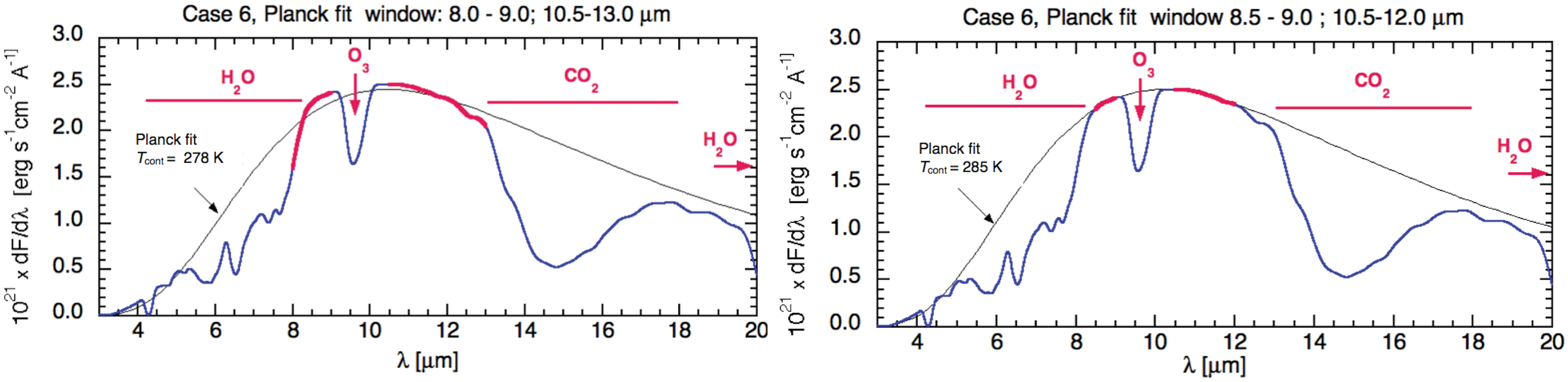
When using the absorption cross sections given in Fig. 1, the usual windows are found in the 8.0–9.0 μm and 10–13 μm domains for an Earth-like atmosphere. To investigate the effect of changing spectral resolution, the spectrum of an Earth-like planet is computed with different window sizes which result (Fig. 2); then the quality of the derived continuum is estimated. It is generally required thereby that spectral features appear in absorption (“downward”) and that the derived temperature is close to that given as input. The Planck function has only two fitting parameters, temperature and amplitude. A least-squares fit is applied to the data points within the different windows. Results indicate that the narrower windows (8.5–9.0 μm, 10.5–12.0 μm) lead to a better-estimated continuum compared with the broader ones (8.0–9.0 μm, 10.5–13.0 μm). The former are then adopted whenever a spectrum looks analogous to that of Earth.

FIG. 2.

Solid blue line: spectra of a Super-earth (M = 4.0 M _earth, R = 1.5 R _earth) in the HZ of eps Eri (S = 1.0 S _earth, 275 K equilibrium temperature). Input atmospheric parameters: P _tot = 1 bar (+ H₂O), 19% O₂, 78.36% N₂, 1000 ppm CO₂. The water abundance profile is from the RH of present Earth. O₃ is calculated with a coupled climate-chemistry model. Two spectral continua are calculated. They are Planck function fits within different spectral windows (thick red lines), and a zero flux condition at 3 μm. Temperature and amplitude are the two free parameters of the fit. Left figure uses (8.0–9.0 μm) and (10.5–13.0 μm) windows; right uses (8.5–9.0 μm) and (10.5–12.0 μm). In each case, a quadratic fit to the data points is done to determine the two parameters, and the resulting Planck function is plotted (thin black line). The resulting continuum temperature is indicated. The narrower windows (right) produce a better fit, probably due to non-negligible absorption of H₂O and CO₂ in the broader windows (Fig. 1). Color images available online at www.liebertpub.com/ast

For H₂-dominated atmospheres (case 4, Fig. 3), the above approach is inappropriate since atmospheric windows down to a surface are lacking. An atmospheric composition close to that of Neptune is assumed in order to simulate the so-called “Mini Gas Planets.” In addition to the zero-flux condition at 3.0 μm, the rise of the spectrum at short wavelengths (3–5 μm) is a main focus since this is a region mainly determined by the temperature of the outer atmosphere, at least for Neptune and the other Solar System giant planets. The (10–11 μm) domain is also a focus because CH₄, a major absorber for the giant planets of our system, has a low absorption in that domain (Fig. 1). This approach is illustrated in Fig. 3 for the case of a mini-Neptune in the HZ of eps Eri.

FIG. 3.

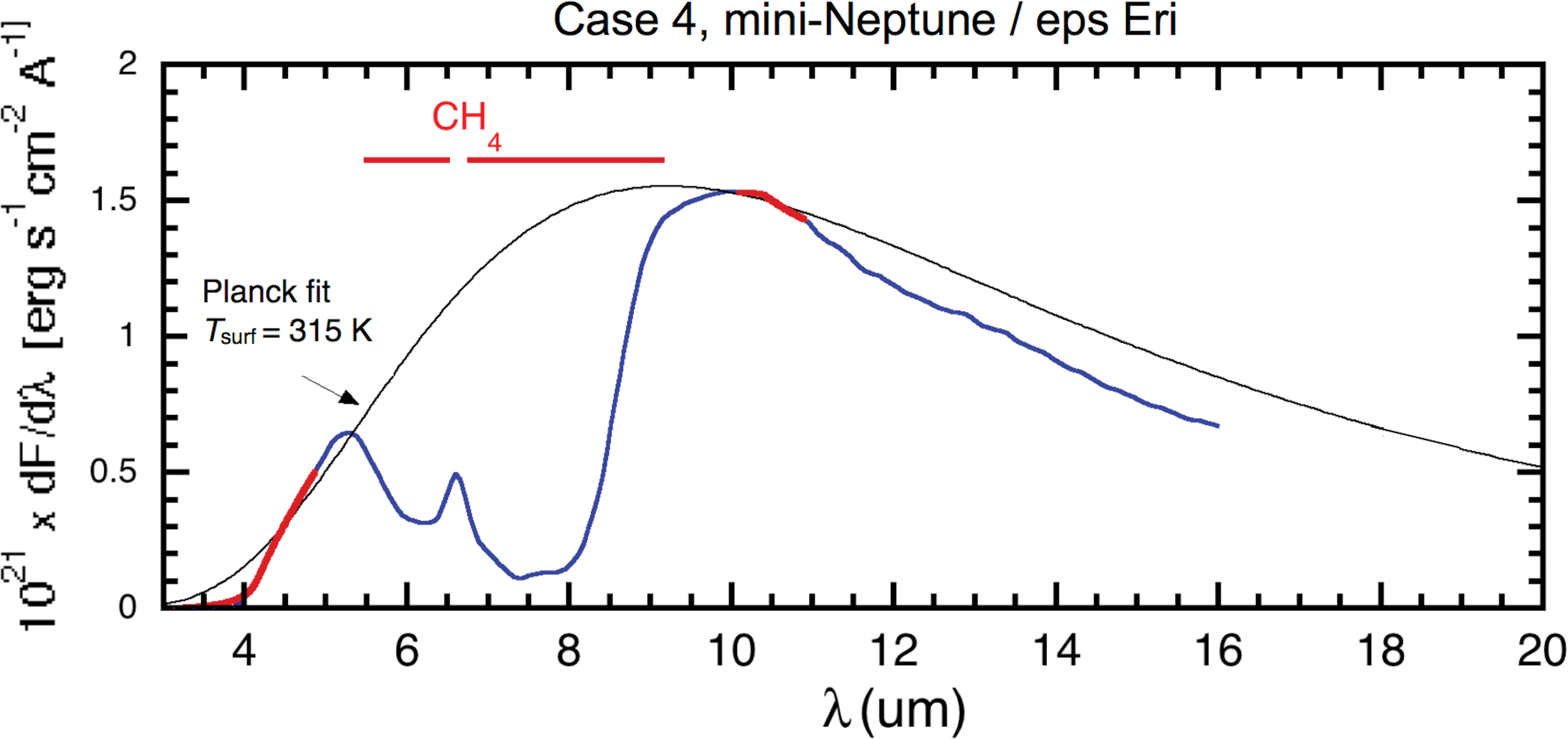
Spectrum (blue line) of a mini-Neptune in the HZ of eps Eri (a = 0.58 AU). Atmospheric composition is 80% H₂, 19% He, 1% CH₄, similar to that of Neptune. Spectral resolution is λ/δλ = 40 at 10 μm. Planck fit is made in the windows stressed by thick red lines. Color images available online at www.liebertpub.com/ast

5. Test Cases

A range of small planets is considered. Several of these constitute possible examples for Proxima Cen b, the planet recently discovered around our nearest star. To explore some diversity regarding the spectral type of the parent star, planets are assumed either to orbit Proxima Cen (M6Ve) or eps Eri (K2V). The mass, radius, and distance to the star are assumed to be observed as should be the case for future missions.

All planets are located within, or close to, the HZ of their star. Their parameters are chosen in order to reflect some diversity, although the examples investigated here are not intended to represent an exhaustive list. The models and parameters used for each case are specified in Table 1.

5.1. Case 1, a rocky planet with no atmosphere orbiting Proxima Cen

The planet is assumed to be rocky with a 4.0 Earth mass and 1.5 Earth radius. For conciseness, these parameters are noted in Earth units: M _pl = 4.0, R _pl = 1.5. Its distance to Proxima Cen is set such that the mean ground temperature is 300 K. A total absorption of the stellar radiation is assumed in the visible–near IR. In the thermal IR, a ground emissivity is chosen to be that of Apollo Moon sample 15071 (Donaldson Hanna et al., 2014; see blue line on the left panel of Fig. 4). The resulting distance to Proxima Cen is 0.043 AU, somewhat closer than the actual Proxima b planet (0.049 AU, Anglada-Escudé et al., 2016).

FIG. 4.

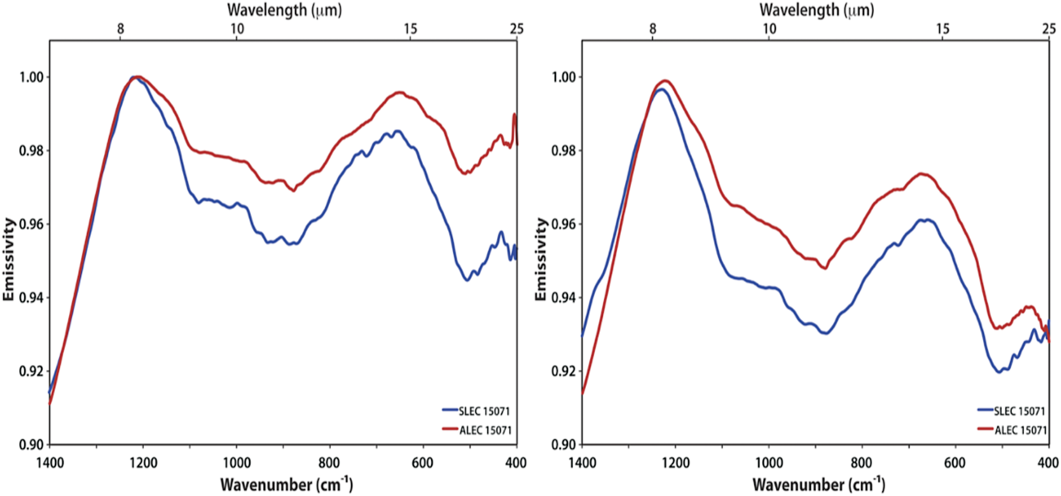
(Left) Ambient emissivity spectra of Apollo 15071 Moon sample measured under ambient conditions (P = 1 bar). (Right) Simulated lunar environment emissivity of the same material (from Donaldson Hanna et al., 2014). SLEC = Simulated Lunar Environment Chamber; ALEC = Asteroidal and Lunar Environmental Chamber. Color images available online at www.liebertpub.com/ast

The computed spectrum and Planck fit are shown in Fig. 5. The spectrum confirms the absence of atmospheric gases. The spectral features of the ground are not confused with usual absorbing gases, thanks to the spectral smoothness of the assumed surface emissivity. A possible interpretation of such a spectrum would be a planet stripped of its atmosphere. Within this framework, the Planck fit provides a good estimate (308 K) of the ground temperature (300 K). Some crude indications as to the nature of surface minerals can be derived from the spectrum, even if the spectral features are very broad (see also Hu et al., 2012, for a related discussion).

FIG. 5.

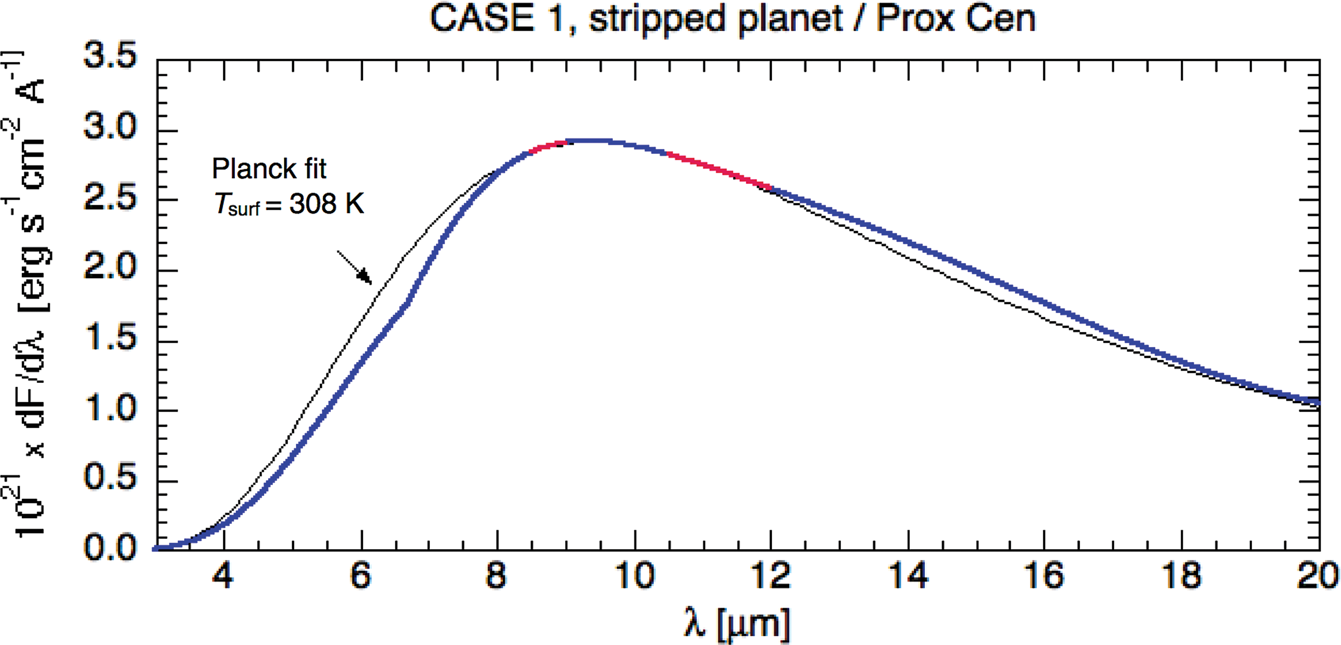
A possible proxy for Proxima b. Solid blue line: computed IR spectrum of a bare rocky planet in the HZ of Prox Cen. The built-in ground temperature is 300 K, and its IR emissivity is that of the Apollo Moon sample 15071 (Donaldson Hanna et al., 2014). Thin black line: Planck fit using data in the wavelength domains in thick red. Color images available online at www.liebertpub.com/ast

5.2. Case 2, a second possible model for Proxima b: A water ocean-planet

A water ocean-planet (Kuchner, 2003; Léger et al., 2004; Selsis et al., 2007) is considered in the HZ of Proxima Cen; the stellar spectrum is assumed to be a M6V Planck curve as in the work of Rauer et al. (2011). Planetary parameters are M = 2.0, R = 1.5 (corresponding to m 50% rocks, 50% water; Selsis et al., 2007).

We assumed Earth insolation in order to investigate the effect of changing the stellar spectrum at constant insolation and calculate T = 280 K surface temperature on applying our climate-chemical model (see Table 1). Higher pressure or/and, for example, larger CO₂ concentrations would be required to obtain a habitable planet at 0.65 S ₀ (as also suggested by previous studies, see, e.g., Turbet et al., 2016). The assumed atmosphere has a 1.2 bar total pressure (+ H₂O), its composition is N₂ 80%, O₂ 20%, plus H₂O assumed to exist at saturation, and very little CO₂ (1 ppm). Note that some O₂, possibly a major part of the total atmospheric inventory, could have resulted from water photolysis by the active star irradiation followed by preferential H escape (Luger and Barnes, 2015; Tian, 2015). We assume O₂ to be abiotic.

The spectrum resulting from the model used (see Table 1) is shown in Fig. 6. It is dominated by H₂O, CO₂, and O₃ absorptions. It looks “Earth-like,” and the corresponding spectral windows are used for the Planck continuum fit (see Section 4). The fit yields a 284 K surface temperature, close to the input one at the liquid-gas interface, 280 K. This is due to the efficient transparency of water vapor in the windows adopted for a planet having a surface at a moderate temperature (at T _surf = 280 K the water vapor pressure is P _surf = 10 mbar at saturation).

FIG. 6.

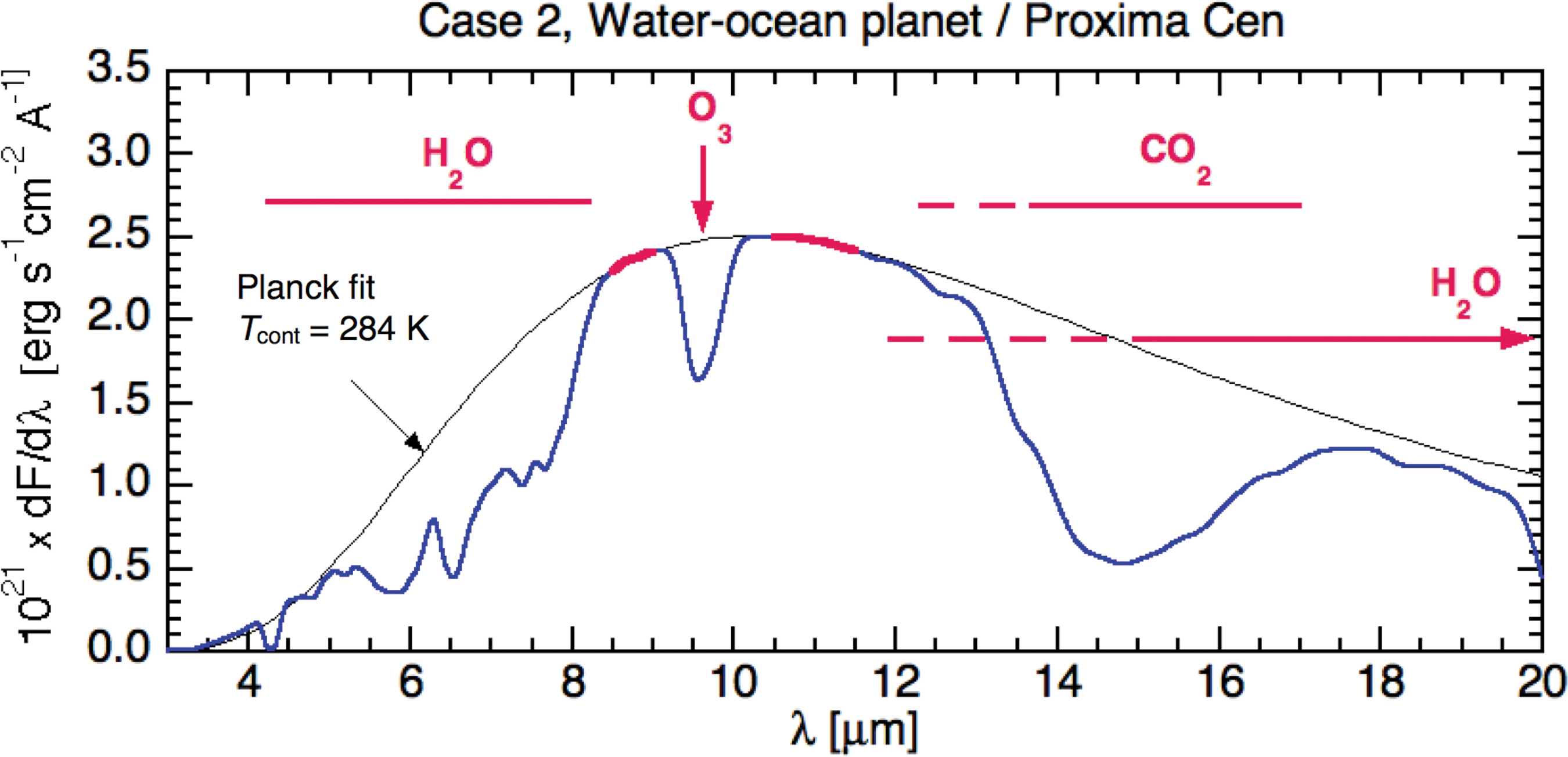
A second possible IR spectrum for Proxima b. Middle thick blue line: calculated spectrum of a water ocean-planet (M _pl = 2.0, R _pl = 1.5, wt. 50% water, 50% rocks) located at 0.049 AU from Proxima Cen (S = 0.65). Input atmosphere: P _N₂ = 1 bar, P _O₂ = 200 mbar, P _CO₂ = 1 μbar, saturated H₂O vapor, T _surface = 290 K. O₃ is calculated with the coupled climate-chemistry models (a) and (b) of Table 1. Spectral resolution is λ/δλ = 40. The Planck fit is performed in the two spectral windows in thick red and the zero flux condition at λ = 3.0 μm. A possible identification of atmospheric species is indicated. Color images available online at www.liebertpub.com/ast

If O₂ is actually abiotic, could this case be considered as a false positive for the triple bioindicator? In the thermal IR detection would be H₂O, CO₂, and O₃. The latter indicates the presence of O₂ but not directly its abundance. Due to feedbacks between UV, O₂, and O₃ and the often-saturated O₃ band, the atmospheric ozone amount remains relatively constant over a wide range of O₂ amounts, namely from 1 PAL (present atmospheric level on Earth) to 10⁻² PAL (Segura et al., 2003). This makes it challenging to determine the abundance of O₂ in this range from observing the O₃. A strong 9.6 μm O₃ band only implies P _O₂ > 1 mbar. A determination could be possible for lower O₂ amounts, for example around 10⁻³ PAL corresponding to a O₃ equivalent width of half its maximum at saturation, based on the modeling scenarios discussed in this paper and assuming CO₂ is sufficiently low (P _CO₂ < 10 mbar) that it does not obscure the O₃ band.

In the present case, a good S/N spectrum of the planet in the visible would allow a precise estimate of the O₂ content, P _O₂ ≈ 250 mbar (as input), and not just P _O₂ > 1 mbar as from the O₃ band in IR. However, in any case the abiotic origin of oxygen would need a study of the impact of a possible water loss and H₂ escape, before applying the triple bioindicator.

This is of special importance for planets in the HZ of any MV star. The latter have a higher luminosity phase at the beginning of their life, when in their pre-main sequence phase, which can result in a large water loss and abiotic O₂ production (Luger and Barnes, 2015; Tian and Ida, 2015).

The planet's water-ocean nature could only be suspected if its bulk density could be estimated at the time when spectroscopy is performed. The planetary radius could be derived from the observed IR spectrum and flux, but its actual mass would require the orbital inclination. Accurate differential astrometry (more than one order of magnitude better than Gaia) could achieve this task and perform a full determination of planetary orbital parameters, including the inclination. Unfortunately, to our knowledge, there is no project planned which will focus on this. This is an important piece of information since any biological modification to the spectrum could be quite different for a water ocean planet compared with a rocky one.

If these two pieces of information—presence of O₂ and planetary density—were available, an intense scientific activity would then be needed to estimate the possible abundance of abiotic O₂ in such an atmosphere, as a result of water photolysis and H escape. It should estimate, or cap: (i) the volcanic source of hydrogen and other reduced gases, and/or other sinks for O₂, for example dissolved ferrous iron in the water ocean; (ii) the oceanic capability to store O₂ 3,4; (iii) the limitations of O₂ abiotic production, including the available FUV flux, stellar evolution, and H₂ diffusion through upper atmosphere.

Our results suggest (see also footnote(3)) that a discussion as to the biological implications of the triple bioindicator could only be considered if one could establish that abiotic process cannot produce P _O₂ ∼250 mbar. Clearly, the observation of a spectrum similar to that of Fig. 6 would trigger exciting exo-geophysical studies.

5.3. Case 3, a third possible case for Proxima b: A rocky super-Earth with biotic O₂ and abundant CO₂

A rocky super-Earth, M = 4.0, R = 1.5, is considered, located at the same distance from Proxima Cen as Proxima b (a = 0.049 AU, S = 0.65). CO₂ is abundant in the atmosphere, P _CO2 = 300 mbar, and its greenhouse effect is assumed to warm the surface up to 280 K. N₂ is present at P _N₂ = 500 mbar, and O₂ at P _O₂ = 200 mbar. Oxygen is assumed biotic, and O₃ is set to modern Earth abundance. The computed spectrum is shown in Fig. 7.

FIG. 7.

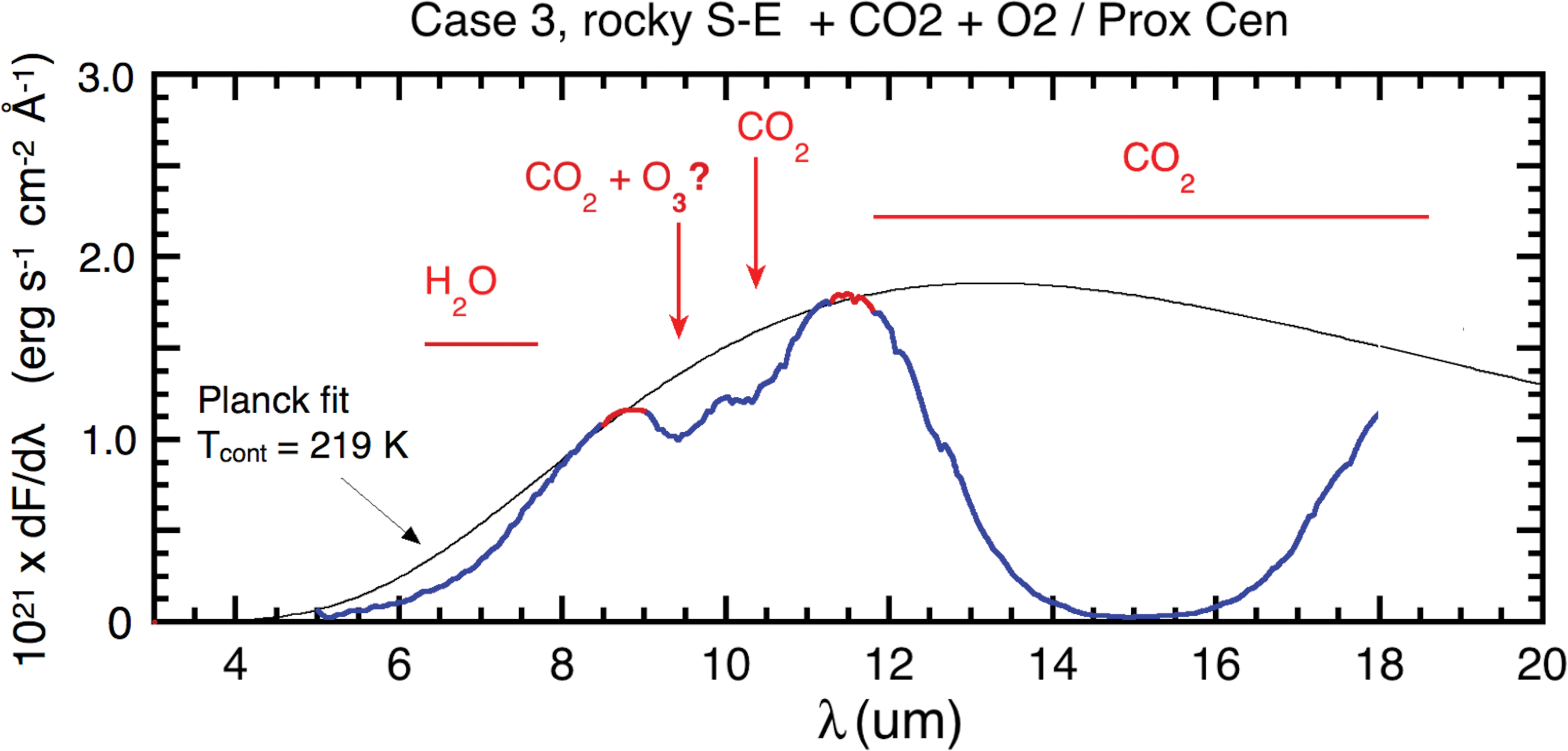
A third possible spectrum (blue line) for Proxima b. A super-Earth, M = 4.0, R = 1.5, is located at 0.049 AU from Prox Cen (S = 0.65) as Proxima b. Atmospheric composition: P _N₂ = 500 mbar, P _CO₂ = 300 mbar, P _O₂ = 200 mbar, H₂O from vapor pressure, O₃ from modeling. Ground temperature is 280 K. Spectral resolution is λ/δλ = 40. As in Fig. 6, the Planck fit is performed in the atmospheric windows stressed in red. It yields T _cont = 219 K. The H₂O and CO₂ band positions are indicated. The possible O₃ band is at the same position as the CO₂ satellite band at 9.4 μm. Color images available online at www.liebertpub.com/ast

The Planck fit yields a temperature of 219 K, which is significantly lower than the ground temperature, 280 K. This is probably due to the poor transparency of the adopted windows when CO₂ is abundant (Fig. 1).

H₂O and CO₂ species are identified. The CO₂ 15 μm band is strong and saturated. The observed band at 10.5 μm is interpreted as a CO₂ satellite feature. It corresponds to a much lower oscillator strength than the 15 μm band, its cross section being 4 orders of magnitude lower (Fig. 1). As it is located in a domain without other major absorption, it allows an estimate of the CO₂ abundance. At the spectral resolution of 40, one measures a ∼20% absorption. From the curve of growth (CoG)⁵ of the band by Des+, this corresponds to a CO₂ pressure of 30 mbar (Fig. 8). This is a lower limit because the spectral resolution is limited, and therefore is consistent with the input 300 mbar⁶.

FIG. 8.

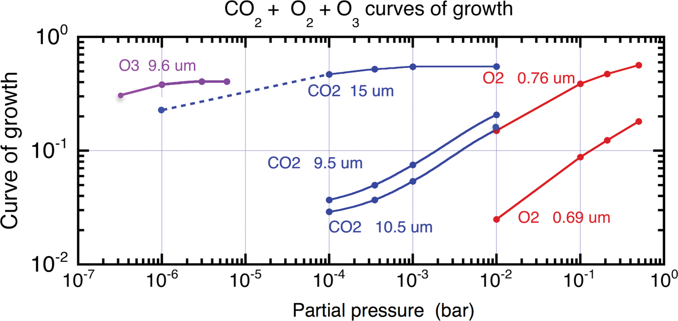
The curve of growth (CoG) of a band is the ratio of its area at a given abundance, divided by its maximum area. It varies as a function of the partial pressure of the responsible gas. Different CoGs of relevant gases are shown for atmospheres without clouds. The O₃ 9.6 μm and CO₂ 15 μm bands are almost saturated for abundances of interest, which results from the large oscillator strength of the corresponding vibrational modes. The other bands are not. Data from Des+. Color images available online at www.liebertpub.com/ast

What is the significance of the 9.5 μm band? At the spectral resolution used, this band overlaps with both an O₃ band (9.6 μm) and a second CO₂ satellite band (9.4 μm) (Fig. 1). According to the preceding estimate of the CO₂ abundance and the CoG of this band, the CO₂ 9.3 μm band alone would have a depth of ∼30%, whereas the observed value is ∼25%. Then, the observed band can be explained by CO₂ only, and there is no evidence of an additional O₃ band that would trace the (actual) presence of O₂. This does not therefore constitute an example of a false negative for the triple bioindicator; it instead constitutes a case where such ideas cannot apply, even for cases where O₂ is abundant in the input atmosphere. Selsis et al. (2002) came to a similar conclusion when assuming P _CO₂ = 1 bar.

The visible spectrum would offer valuable information when investigating this scenario. This could indicate the presence of O₂ and its approximate abundance using a modeling of the atmosphere, including its clouds. These two pieces of information cannot been deduced from the IR spectrum in this particular case, because the O₃ band is hidden by a CO₂ satellite band.

In the Earth visible spectrum, with P _O₂ = 210 mbar, the 0.76 μm O₂ band is 50% deep for an average cloud coverage, and the 0.69 μm band feature is 19% (Des+). Although the reflectance spectrum of the considered planet has not been calculated in the present work, it is likely that the spectral features would be analogous for this super-Earth (M = 4.0, R = 1.5) and Earth because the main difference between their atmospheres is their scale heights (proportional to R _pl). Most of the O₂ bands are not saturated, and if the S/N ratio of the visible spectrum is sufficient, they would allow a good estimate of the abundance of O₂. This remains true in the worst-case scenario assuming full cloud coverage⁷ because O₂ is also present in the high atmosphere, above the water clouds⁸. Detecting a high O₂ abundance would be an indication that it is biotic because the abiotic source due to CO₂ photolysis is considered as negligible (Section 5.6). However, only a high-quality spectrum in the visible could achieve the above, typically with λ/δλ ≥ 70 and S/N ≥ 8 for a 4σ detection of the strongest O₂ band.

This represents a case where the simultaneous observation of both spectral domains (thermal IR + visible), with good spectral resolution and S/N, is desirable.

5.4. Case 4, a mini-Neptune in the HZ of Epsilon Eridani

In Case 4, and subsequent cases, planets are considered around the solar-type star, Epsilon Eridani (eps Eri). A mini-Neptune (M = 4.0, R = 1.8) is located in the HZ of eps Eri at a = 0.58 AU (S = 1.0). The atmosphere is made up of 80% H₂, 19% He, and 1% CH₄, close to that of Neptune (3%) or the other gaseous planets of the Solar System (Guillot and Gautier, 2007). The resulting spectrum is shown in Fig. 3, Section 4. The Planck continuum is fitted to a zero flux at 3.0 μm, and data in (4–5 μm) and (10–11 μm) windows. The “surface” temperature found is 315 K.

Strong and broad absorption features appear around 6.0 and 7.5 μm⁹. They are attributed to CH₄, as in Neptune (Fletcher et al., 2010). They correspond to strong bands in the CH₄ spectrum (Fig. 1). The 7.5 μm feature corresponds to the umbrella bending mode of this molecule. The observed spectrum is consistent with a H₂-rich atmosphere, provided its upper parts contain CH₄ as in all the giant planets of the Solar System (CH₄ parts by volume are Jupiter ∼0.2%, Saturn ∼0.4%, Neptune ∼3%, Uranus ∼3%; Guillot and Gautier, 2007).

5.5. Case 5, a hot water ocean-planet around Epsilon Eridani

A water ocean-planet, M _pl = 2.0, R _pl = 1.5 (mass 50% water, 50% rocks), is similar to that of Case 2, but orbiting around eps Eri and significantly hotter, a = 0.57, S = 1.05. Atmospheric abundances are P _N2 = 1 bar, H₂O from saturated vapor, 1 ppm CO₂, no O₂. At liquid/vapor interface, the climate model gives T = 413 K and P _H₂O = 3.6 bar. The H₂O greenhouse effect is quite strong even if the insolation increase is rather modest compared to the Earth case. This is because (i) we assume 100% relative humidity, and (ii) the incoming radiation wavelengths are skewed redward compared to the Solar case (see e.g. Godolt et al. 2016). The situation is somewhat analogous to that of Venus where the strong CO₂ greenhouse effect brings the planetary surface to a temperature much higher than on Earth, even if the solar energy absorbed per unit surface of the planet is lower than on our planet as a result of a higher albedo.

The calculated spectrum is shown in Fig. 9. Contrary to the preceding cases, the Planck fit does not use several data points within atmospheric windows, but instead employs only a few discrete points in order to obtain a continuum from which all features appear downward. This situation is due to the strong absorption of the thick H₂O atmosphere. Selected points are dF/dλ (2 μm) = 0, the 2 μm wavelength is selected rather than 3 μm to take into account the likely high surface temperature; dF/dλ (3.75 μm) is set to a data point which corresponds to a local minimum in the water absorption spectrum; dF/dλ (12.2 μm) is set to another data point corresponding to a deep minimum for both H₂O and CO₂ (Fig. 1). With these points, the fit yields a surface temperature, T _cont = 415 K, that is close to the input value (413 K) at the ocean surface. This agrees with the low cross sections of H₂O vapor at these two wavelengths. Note that the total pressure at the ocean surface is ≈4.6 bar.

FIG. 9.

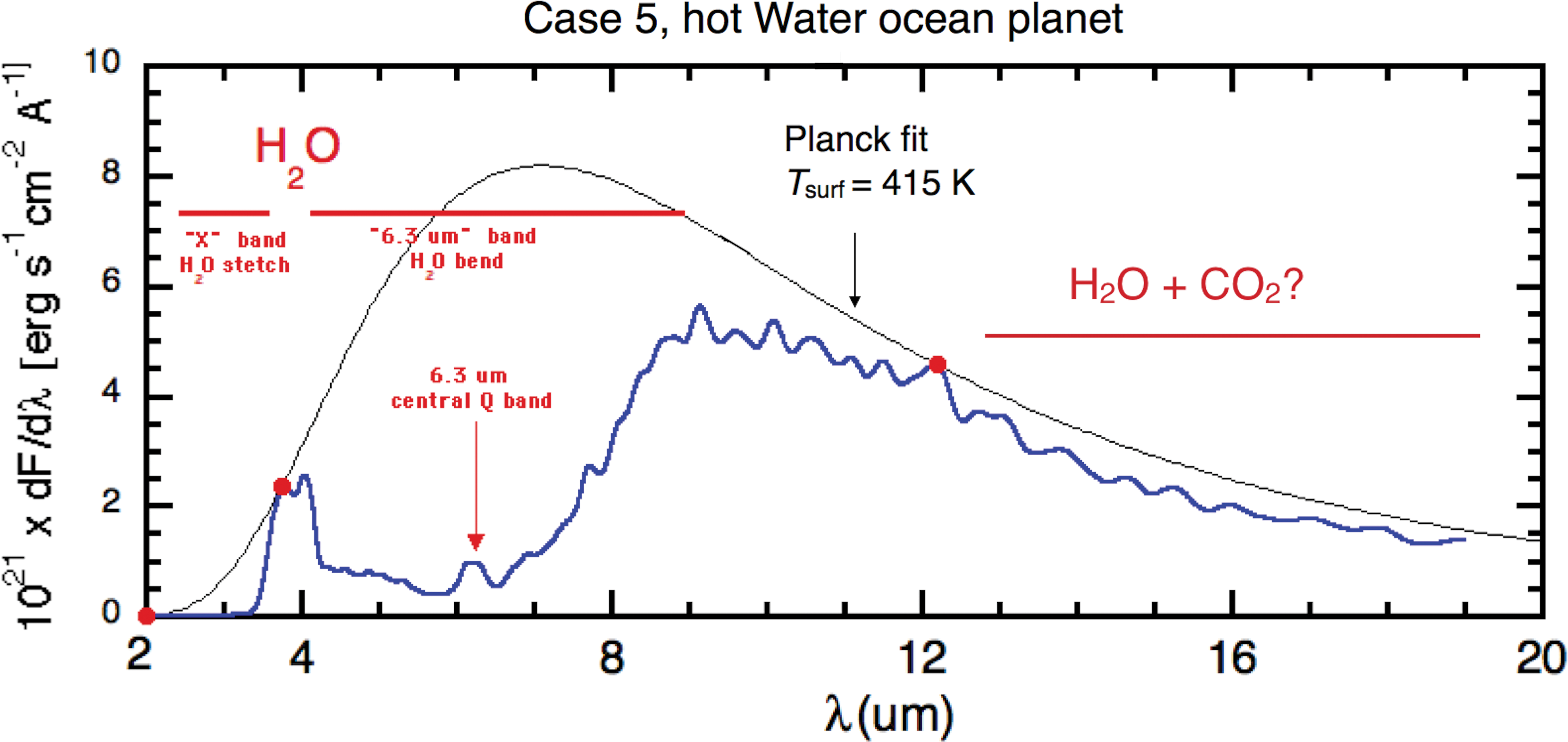
A hot water ocean-planet (M _pl = 2.0, R _pl = 1.5) at a = 0.57 AU of eps Eri (S = 1.05). Input atmosphere: P _N₂ = 1 bar, H₂O from saturated vapor, 1 ppm CO₂, no O₂. The calculated spectrum is at resolution λ/δλ = 40. The Planck fit is obtained from the three isolated data points in thick red. Identifications of species are indicated. Color images available online at www.liebertpub.com/ast

A deep absorption is observed in the (4.2–9.0 μm) interval, corresponding to the P and R parts of the so-called “6.3 μm” bending mode of water. The central Q band appears as a reduction in the absorption, in agreement with the lower cross section at that wavelength (Fig. 1). The flux decrease at λ < 3.75 μm is steeper than that of the Planck function and reveals the absorption of the H₂O double stretching modes (so-called “X” band).

The CO₂ absorption around 15 μm is still marginally evident, even at such an assumed low abundance of the gas. The assumed data (with no noise sources) suggest that detailed modeling could permit its detection, especially since H₂O absorption is low in the (12–17 μm) domain and would not overlap with the CO₂ absorption. However, with actual data on the sky and including realistic noise sources, CO₂ detection would probably be difficult unless one achieves a high signal-to-noise ratio (S/N ≳ 20).

A measurement of the mass of the planet would be mandatory to establish its water-ocean nature and distinguish it from a hot rocky planet with much less water and possibly emerged continents. This would be necessary to derive any inference that could be relevant for exobiology.

5.6. Case 6, a super-Earth in the HZ of Epsilon Eridani, with O₂

The planet here considered is analogous to Earth but larger, M = 4, R = 1.5. It orbits around eps Eri at a distance a = 0.58 AU, so that S = 1.0. The atmospheric composition is similar to that of our home planet: P _tot = 1 bar (+ H₂O); 78.4% N₂; 19% O₂; H₂O from vapor pressure and relative humidity profile from that of present Earth (Manabe and Wetherald, 1967); 1000 ppm CO₂. O₂ is assumed biotic as in Case 3. The larger gravity (17.5 m s⁻²) makes the atmospheric scale, h, smaller than that of Earth.

In this case, climate-chemistry and radiative transfer emission calculations are performed (Table 1). Results are shown in Fig. 10.

FIG. 10.

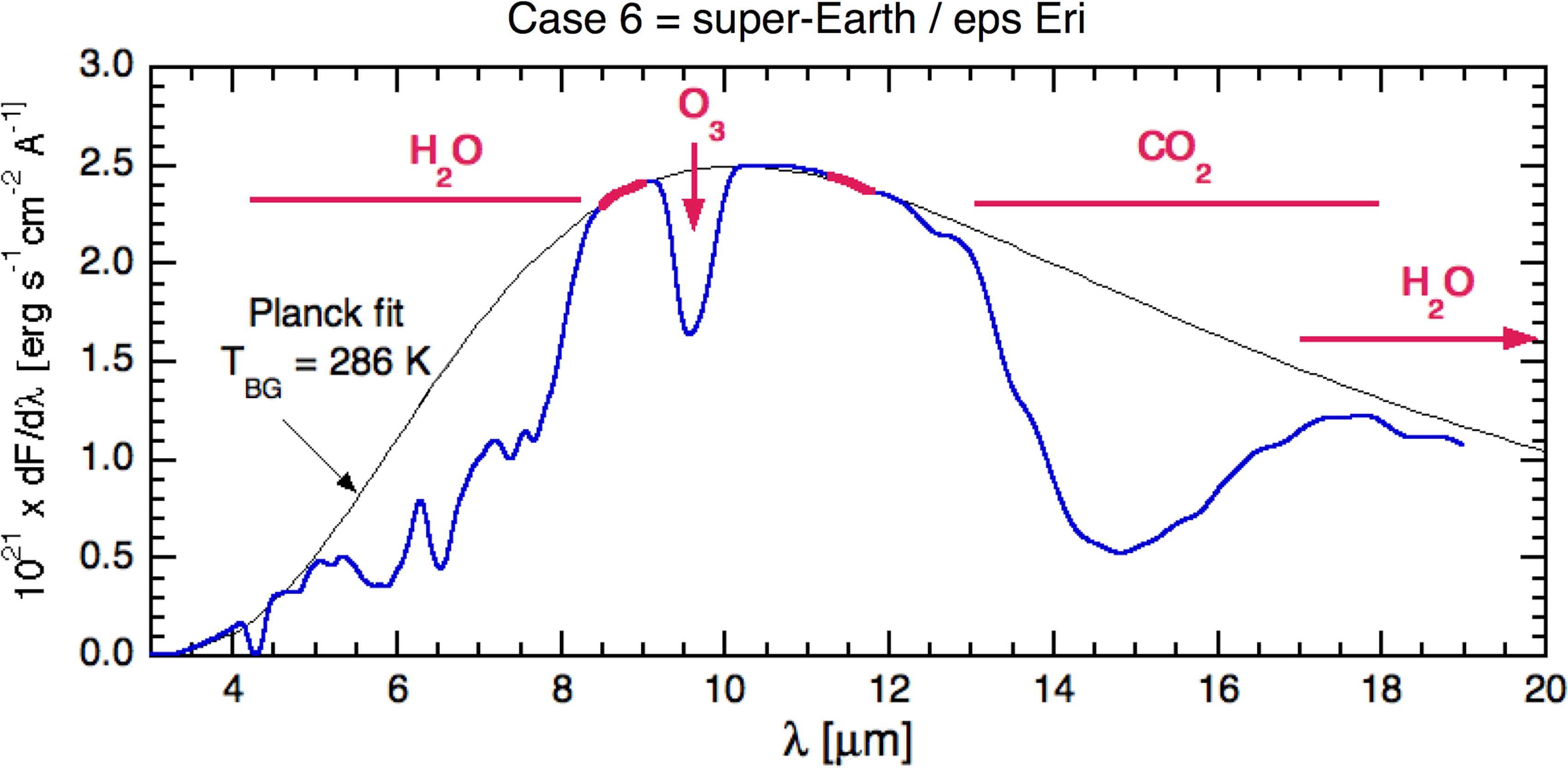
A super-Earth spectrum is calculated (solid blue) at λ/δλ = 40. The planet is in the HZ of eps Eri (S = 1.0, T _eq = 275 K). Atmospheric features are P _tot = 1 bar (+ H₂O), 19% O₂, 78% N₂, 1000 ppm CO₂, water abundance and profile from the RH profile of present Earth. O₃ is calculated by the coupled climate-chemistry model (a) and (b) of Table 1. The windows used for the Planck fit are in thick red lines. H₂O, CO₂, and O₃ bands are detected. Color images available online at www.liebertpub.com/ast

The Planck continuum gives T _cont = 286 K, and spectral features of H₂O, O₃, and CO₂ are observed. The 9.6 μm O₃ band is saturated, which indicates P _O₂ > 1.0 mbar for a K2V star (Segura et al., 2003).

Does this spectrum reveal possible biogenic activity on the planet? In other words, does the triple bioindicator apply? The abiotic production of O₂ by CO₂ photolysis was suggested to be capped at ∼10 mbar for planets in the HZ of dwarf stars and especially for MV (Rosenqvist et al., 1995; Tian et al., 2014), but this value has been recently reduced by 3 orders of magnitude (< 10 μbar) for FGK and M stars in a study by Harman et al. (2018)¹⁰. This lower O₂ threshold is explained by the CO and O recombination catalyzed by the nitrogen oxides NO_x produced in lightning¹¹, for atmospheres with significant N₂ abundance (> 1%).

Considering the large difference between the P _O2 estimate from the spectrum (1.0 mbar) and the expected abiotic maximum production (10 μbar), we conclude that the triple bioindicator applies correctly.

6. What Spectral Resolution, What Signal-to-Noise Ratio?

So far, most analyses have been performed with a spectral resolution λ/δλ = 40, and an infinite S/N, which is of course unobtainable in practice. Here, an optimal set of values for (λ/δλ, S/N) will be searched for.

For a given target, the required integration time to detect a spectral feature depends on its relative depth from the continuum, spectral resolution λ/δλ, and S/N on the continuum (see the caption to Fig. 11 for a precise definition of S and N). The larger these parameters, the better the discrimination capability but the longer the required integration time t _int. A compromise is necessary.

FIG. 11.

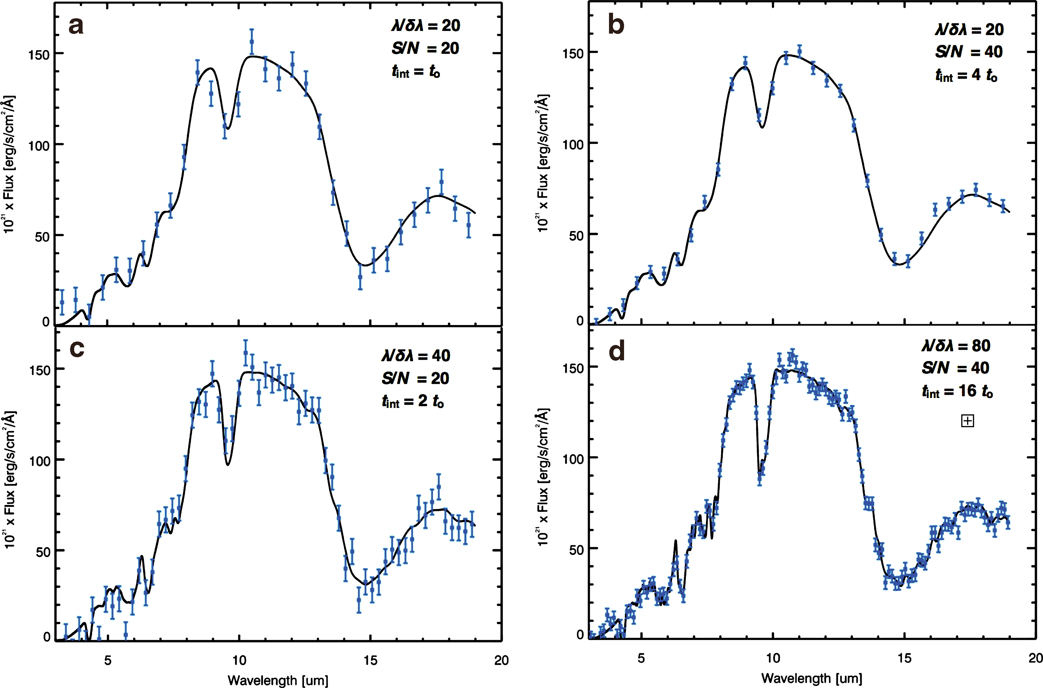
Four calculated spectra of a super-Earth in order to determine good acquisition parameters. From case (a) to (d), different sets of spectral resolution and S/N at 10 μm are used. The atmospheric composition is similar to that of our Earth, and the parent star is eps Eri. Each panel corresponds to a given λ/δλ and S/N. S is the flux in the continuum at 10 μm, and N = σ is the standard deviation of a random function independent of λ, which is added to each data point. Blue dots and bars mimic observations. Dots are located on an arbitrary wavelength grid with intervals 1.0 δλ (no oversampling). Fluxes correspond to the outcome of the climate model plus a random function. Total bar amplitudes are 2σ. For each plot, selected λ/δλ, S/N, and required integration time t _int are indicated. The latter are expressed as multiples of t _o, the integration time of case (a). Color images available online at www.liebertpub.com/ast

The Earth-like spectrum of Case 6 is chosen with such a compromise in mind. The main spectral features are due to CO₂, H₂O, and O₃. They can be observed at different spectral resolutions and S/N. Figure 11 shows four spectra calculated with different combinations of these two parameters, and the corresponding integration times.

To qualify the detection of a band, the following criteria are used.

Spectral resolution: at least two data points should be in the FWHM of the band, whatever the relative position of the wavelength grid with respect to the band.

Signal-to-noise ratio: if A _band is the band depth relative to the continuum, and σ _comb is the standard deviation when combining all the data points within the band, the relation A _band/σ _comb > 5 should be satisfied.

Considering the key O₃ band, a set of parameters is searched for that fulfills these two criteria at a minimum time cost. Table 2 summarizes the parameter sets and indicates whether the criteria are met.

Table 2.

Analysis of O₃ Bands Present in Figure 11

Panel	λ/δλ	(S/N)_data	t _int/t₀	2 data points in FWHM for any grid?	(S/N)_band = A _band/σ_comb
(a)	20	20	1	No	8
(b)	20	40	4	No	16
(c)	40	20	2	Yes	16
(d)	80	40	16	Yes	45

Among the four sets, set (c) (λ/δλ = 40, S/N = 20) meets both criteria for a minimum integration time. It is proposed as a compromise.

It is interesting to compare set (c) and set (b). The highest spectral resolution one (c), fulfills both criteria (1) and (2). It corresponds to an integration time t _int = 2t ₀. The highest signal-to-noise one (b), λ/δλ = 20, S/N = 40, does not fulfill criteria (1), even if its integration time is twice as long, t _int = 4t ₀. At least in that case, high spectral resolution is preferable to high signal to noise.

In the same way, a detailed study by von Paris et al. (2013) concluded that λ/δλ = 20, S/N = 10 do not allow reliable detections of H₂O nor O₃, in Earth-like IR spectra, which agrees with our proposed values.

This suggests an instrumental strategy: one should attempt to build an instrument with a spectral resolution that satisfies criteria (1) for all bands of interest. It should retain the possibility of working at high spectral resolution whenever desirable. For broader bands, binning data points for faster observations will always be possible, whereas if the instrumental resolution is low the reverse would not be possible. For detectors the requirement is classical; they should have dark current and read-out noise low enough so that the total noise is dominated by photon noise for most, if not all, observations.

7. Summary and Conclusion

An exercise was performed for testing the ability of thermal IR spectroscopy to retrieve key components of the atmosphere of a few putative exoplanets, some being different possible cases for the Proxima b planet. All were assumed to be in the HZ of their star, or close to it, according to a special interest in the search for planets where water can be liquid, and the triple bioindicator (H₂O, CO₂, O₂, under specified conditions) criteria is considered. Covering an extensive diversity range has guided our choice of planets, including diversity in their bulk properties (rocky, water-ocean, hydrogen rich), atmospheric compositions, and spectral types of the parent star.

Planets were considered to have an a priori atmospheric composition. Coupled climate-chemistry, and climate-only calculations have been carried out for three cases. The coupled climate-chemistry also calculated minor species that can be produced by photochemistry, including O₃. In two others the atmospheric structure was imposed; in a sixth one we assumed a planet without atmosphere and prescribed the surface emissivity. The IR emission was computed by using line-by-line radiative transfer models, and the ability to retrieve input gases and climate parameters was then investigated.

For the six putative planets considered, no false positive of the triple bioindicator is found considering, e.g., the impact of the harsh irradiations from a M6Ve star and possible O₂ buildup, due to H₂O photolysis and H₂ escape during the hot early phase of the stellar evolution. Notably, in Case 3, a telluric planet with O₂ and abundant CO₂, the abundant presence of the latter gas prevents the observation of the 9.6 μm O₃ band and consequently the detection of O₂. In Case 4, the spectrum of an assumed H₂-rich planet pointed correctly to the identification of a gaseous planet.

In some cases, the simultaneous acquisition of a visible spectrum would be necessary, especially when CO₂ is abundant (P _CO₂ > 300 mbar), so that its satellite band at 9.4 μm hides the 9.6 μm O₃ band in the thermal IR (Case 3). In all cases, high S/N spectra in the visible domain can give additional information/confirmation, which would be valuable for our understanding of local conditions.

Finally, the measurement of the mass of the planet is mandatory in all cases for identifying its bulk composition and having an idea of the conditions at the surface, necessary conditions for any spectroscopic bioindicator study. It is pointed out that no space mission, nor ground observation, is foreseen that can perform this task exhaustively for our neighboring stars, the targets of future spectroscopic observations.

An observing strategy is proposed for the retrieval of key species at a minimum integration time cost, a spectral resolution λ/δλ = 40, and a signal-to-noise ratio S/N = 20. It fulfills criteria for the detection of the main species in Earth-like spectra. This approach is preferred over the more costly λ/δλ = 20 and S/N = 40, which does not always fulfill detection criteria and requires longer integration times. In summary, there is an important take-home message arising from our study: future-planned instruments require a spectral resolution of at least 40.

Footnotes

Abbreviations Used

References

Angel

J.R.

, Cheng

A.Y.

, and Woolf

N.J.

(1986) A space telescope for IR spectroscopy of Earth-like planets. Nature, 322:341–343.

Anglada-Escudé

, Amado

P.J.

, Barnes

, Berdiñas

Z.M.

, Butler

R.P.

, Coleman

G.A.

, de la Cueva

, Dreizler

, Endl

, Giesers

, Jeffers

S.V.

, Jenkins

J.S.

, Jones

H.R.

, Kiraga

, Kürster

, López-González

M.J.

, Marvin

C.J.

, Morales

, Morin

, Nelson

R.P.

, Oritz

J.L.

, Ofir

, Paardekooper

S.-J.

, Reiners

, Rodríguez

, Rodríguez-López

, Sarmiento

L.F.

, Strachan

J.P.

, Tsapras

, Tuomi

, and Zechmeister

(2016) A terrestrial planet candidate in a temperate orbit around Proxima Centauri. Nature, 536:437–440.

Catling

D.C.

and Kasting

J.F.

(2017) Atmospheric Evolution on Inhabited and Lifeless Worlds, Cambridge University Press, Cambridge, UK.

Des Marais

D.J.

, Harwit

M.O.

, Jucks

K.W.

, Kasting

J.F.

, Lin

D.N.C.

, Lunine

J.I.

, and Woolf

N.J.

(2002) Remote sensing of planetary properties and biosignatures on extrasolar terrestrial planets. Astrobiology, 2:153–181.

Donaldson Hanna

K.L.

, Thomas

I.R.

, Greenhagen

B.T.

, Bowles

N.E.

, and Pieters

C.M.

(2014) Characterization of Apollo soil samples under simulated lunar conditions [abstract 2345]. In 45^th Lunar and Planetary Science Conference, Lunar and Planetary Institute, Houston.

Fletcher

L.N.

, Drossart

, Burgdorf

, Orton

G.S.

, and Encrenaz

(2010) Neptune's atmospheric composition from AKARI infrared spectroscopy. Astron Astrophys, 514:A17.

García Muñoz

and Isaak

K.G.

(2015) Probing exoplanet clouds with optical phase curves. Proc Natl Acad Sci USA, 112:13461–13466.

García Muñoz

, Wolkenberg

, Sanchez-Lavega

, Huesco

, and Garate-Lopez

(2013) A model of scattered thermal radiation for Venus from 3 to 5 μm. Planet Space Sci, 81:65–73.

Godolt

, Grenfell

J.L.

, Kitzmann

, Kunze

, Langematz

, Patzer

A.B.C.

, Rauer

, and Stracke

(2016) Assessing the habitability of planets with Earth-like atmospheres with 1D and 3D climate modeling. Astron Astrophys, 592:A36.

10.

Grenfell

J.L.

(2017) A review of exoplanetary biosignatures. Phys Rep, 713:1–17.

11.

Grenfell

J.L.

, Stracke

, von Paris

, Patzer

, Titz

, Segura

, and Rauer

(2007) The response of atmospheric chemistry on Earthlike planets around F, G and K stars to small variations in orbital distance. Planet Space Sci, 55:661–671.

12.

Guillot

and Gautier

(2007) Giant planets. In Treatise of Geophysics, Vol. 10, Planets and Moons, edited by G. Schubert and T. Spohn, Elsevier, Amsterdam, pp 439–464.

13.

Harman

C.E.

, Felton

, Hu

, Domagal-Goldman

S.D.

, Segura

, Tian

, and Kasting

J.F.

(2018) Abiotic O₂ levels on planets around F, G, K, and M stars: effects of lightning-produced catalysts in eliminating oxygen false positives. Astrophys J, 866, doi:10.3847/1538-4357/aadd9b.

14.

Hatzes

A.P.

, Cochran

W.D.

, McArthur

, Baliunas

S.L.

, Walker

G.A.H.

, Campbell

, Irwin

A.W.

, Yang

, Kürster

, Endl

, Els

, Butler

R.P.

, and Marcy

G.W.

(2000) Evidence for a long-period planet orbiting ɛ Eridani. Astrophys J, 544:L145–L148.

15.

, Seager

, and Bains

(2012) Photochemistry in terrestrial exoplanet atmospheres. I. Photochemistry model and benchmark cases. Astrophys J, 761, doi:10.1088/0004-637X/761/2/166.

16.

Humlíček

(1982) Optimized computation of the Voigt and complex probability functions. J Quant Spectrosc Radiat Transf, 27:437–444.

17.

Kaltenegger

(2017) How to characterize habitable worlds and signs of life. Annu Rev Astron Astrophys, 55:433–485.

18.

Kane

S.R.

, Gelino

D.M.

, and Turnbull

M.C.

(2017) On the orbital inclination of Proxima Centauri b. Astrophys J, 153, doi:10.3847/1538-3881/153/2/52.

19.

Kasting

J.F.

(1995) O₂ concentrations in dense primitive atmospheres: commentary. Planet Space Sci, 43:11–13.

20.

Kiang

N.Y.

, Domagal-Goldman

, Parenteau

M.N.

, Catling

D.C.

, Fujii

, Meadows

V.S.

, Schwieterman

E.W.

, and Walker

S.I.

(2018) Exoplanet biosignatures: at the dawn of a new era of planetary observations. Astrobiology, 18:619–629.

21.

Kopparapu

R.K.

(2013) A revised estimate of the occurrence rate of terrestrial planets in the habitable zones around Kepler M-dwarfs. Astrophys J, 767, doi:10.1088/2041-8205/767/1/L8.

22.

Kreidberg

and Loeb

(2016) Prospects for characterizing the atmosphere of Proxima Centauri b. Astrophys J, 832:L12.

23.

Kuchner

(2003) Volatile-rich Earth-mass planets in the habitable zone. Astrophys J, 596:L105.

24.

Léger

, Selsis

, Sotin

, Guillot

, Despois

, Mawet

, Ollivier

, Labèque

, Valette

, Brachet

, Chazelas

, and Lammer

(2004) A new family of planets? “Ocean-Planets.”. Icarus, 169:499–504.

25.

Léger

, Fontecave

, Labeyrie

, Samuel

, Demangeon

, and Valencia

(2011) Is the presence of oxygen on an exoplanet a reliable biosignature?. Astrobiology, 11:335–341.

26.

, Tian

, Wang

Y.W.

, Wei

W.J.

, and Huang

X.M.

(2016) Distinguishing a hypothetical abiotic planet–moon system from a single inhabited planet. Astrophys J, 817:L15.

27.

Luger

and Barnes

(2015) Extreme water loss and abiotic O₂ buildup on planets throughout the habitable zones of M dwarfs. Astrobiology, 15:119–143.

28.

Manabe

and Wetherald

R.T.

(1967) Thermal equilibrium of the atmosphere with a given distribution of relative humidity. J Atmos Sci, 24:241–259.

29.

Martins

J.H.C.

, Figueira

, Santos

N.C.

, Melo

, Garcia- Muñoz

, Faria

, and Pepe

(2018) Recovering the colour-dependent albedo of exoplanets with high-resolution spectroscopy: from ESPRESSO to the ELT. Mon Not R Astron Soc, 478:5240–5262.

30.

Meadows

V.S.

, Arney

G.N.

, Schwieterman

E.W.

, Lustig-Yaeger

, Lincowski

A.P.

, Robinson

, Domagal-Goldman

S.D.

, Deitrick

, Barnes

R.K.

, Fleming

D.P.

, Luger

, Driscoll

P.E.

, Quinn

T.R.

, and Crisp

(2018a) The habitability of Proxima Centauri b: environmental states and observational discriminants. Astrobiology, 18:133–189.

31.

Meadows

V.S.

, Reinhard

C.T.

, Arney

G.N.

, Parenteau

M.N.

, Schwieterman

E.W.

, Domagal-Goldman

, Lincowski

A.P.

, Stapelfeldt

K.R.

, Rauer

, DasSarma

, Hegde

, Narita

, Deitrick

, Lustig-Yaeger

, Lyons

T.W.

, Siegler

, and Grenfell

J.L.

(2018b) Exoplanet biosignatures: understanding oxygen as a biosignature in the context of its environment. Astrobiology, 18:630–662.

32.

Rauer

, Gebauer

, Paris

P.V.

, Cabrera

, Godolt

, Grenfell

J.L.

, Belu

, Selsis

, Hedelt

, and Schreier

(2011) Potential biosignatures in super-Earth atmospheres I. Spectral appearance of super-Earths around M dwarfs. Astron Astrophys 529:A8.

33.

Rein

, Fujii

, and Spiegel

D.S.

(2014) Some inconvenient truths about biosignatures involving two chemical species on Earth-like exoplanets. Proc Natl Acad Sci USA, 111:6871–6875.

34.

Rieke

G.H.

(2009) History of infrared telescopes and astronomy. Experimental Astronomy, 25:125–141.

35.

Rosenqvist

and Chassefiere

(1995) Inorganic chemistry of O₂ in a dense primitive atmosphere. Planet Space Sci, 43:3–10.

36.

Rothman

L.S.

, Gordon

I.E.

, Babikov

, Barbe

, Chris Benner

, Bernath

P.F.

, Birk

, Bizzocchi

, Boudon

, Brown

L.R.

, Campargue

, Chance

, Cohen

E.A.

, Coudert

L.H.

, Devi

V.M.

, Drouin

B.J.

, Fayt

, Flaud

J.-M.

, Gamache

R.R.

, Harrison

J.J.

, Hartmann

J.-M.

, Hill

, Hodges

J.T.

, Jacquemart

, Jolly

, Lamouroux

, LeRoy

R.J.

, Li

, Long

D.A.

, Lyulin

O.M.

, Mackie

C.J.

, Massie

S.T.

, Mikhailenko

, Müller

H.S.P.

, Naumenko

O.V.

, Nikitin

A.V.

, Orphal

, Perevalov

, Perrin

, Polovtseva

E.R.

, Richard

, Smith

M.A.H.

, Starikova

, Sung

, Tashkun

, Tennyson

, Toon

G.C.

, Tyuterev

.G., and Wagner

(2013) The HITRAN2012 molecular spectroscopic database. J Quant Spectrosc Radiat Transf, 130:4–50.

37.

Schwieterman

E.W.

, Kiang

N.Y.

, Parenteau

M.N.

, Harman

C.E.

, DasSarma

, Fisher

T.M.

, Arney

G.N.

, Hartnett

H.E.

, Reinhard

C.T.

, Olson

S.L.

, Meadows

V.S.

, Cockell

C.S.

, Walker

S.I.

, Grenfell

J.L.

, Hegde

, Rugheimer

, Hu

, and Lyons

T.W.

(2018) Exoplanet biosignatures: a review of remotely detectable signs of life. Astrobiology, 18:663–708.

38.

Segura

, Krelove

, Kasting

J.F.

, Sommerlatt

, Meadows

, Crisp

, Cohen

, and Mlawer

(2003) Ozone concentrations and ultraviolet fluxes on Earth-like planets around other stars. Astrobiology, 3:689–708.

39.

Selsis

, Despois

, and Parisot

J.-P.

(2002) Signature of life on exoplanets: can Darwin produce false positive detections?. Astron Astrophys, 388:985–1003.

40.

Selsis

, Chazelas

, Bordé

, Ollivier

, Brachet

, Decaudin

, Bouchy

, Ehrenreich

, Grießmeier

J.-M.

, Lammer

, Sotin

, Grasset

, Moutou

, Barge

, Deleuil

, Mawet

, Despois

, Kasting

J.F.

, and Léger

(2007) Could we identify hot ocean-planets with CoRoT, Kepler and Doppler velocimetry?. Icarus, 191:453–468.

41.

Stamnes

, Tsay

S.C.

, Wiscombe

, and Jayaweera

(1988) Numerically stable algorithm for discrete-ordinate-method radiative transfer in multiple scattering and emitting layered media. Appl Opt, 27:2502–2509.

42.

Tian

(2015) History of water loss and atmospheric O₂ buildup on rocky exoplanets near M dwarfs. Earth Planet Sci Lett, 432:126–132.

43.

Tian

and Ida

(2015) Water contents of Earth-mass planets around M dwarfs. Nat Geosci, 8:177–180.

44.

Tian

, France

, Linsky

J.L.

, Mauas

P.J.D.

, and Vieytes

M.C.

(2014) High stellar FUV/NUV ratio and oxygen contents in the atmospheres of potentially habitable planets. Earth Planet Sci Lett, 385:22–27.

45.

Toon

O.B.

, McKay

C.P.

, Ackerman

T.P.

, and Santhanam

(1989) Rapid calculation of radiative heating rates and photodissociation rates in inhomogeneous multiple scattering atmospheres. J Geophys Res: Atmospheres, 94:16287–16301.

46.

Turbet

, Leconte

, Selsis

, Bolmont

, Forget

, Ribas

, Raymond

, and Anglada-Escude

(2016) The habitability of Proxima Centauri b II. Possible climates and observability. Astron Astrophys, 596:A112.

47.

von Paris

, Gebauer

, Godolt

, Grenfell

J.L.

, Hedelt

, Kitzmann

, Patzer

A.B.C.

, Rauer

, and Stracke

(2010) The extrasolar planet Gliese 581d: a potentially habitable planet?. Astron Astrophys, 522:A23.

48.

von Paris

, Hedelt

, Selsis

, and Schreier

(2013) Characterization of potentially habitable planets: retrieval of atmospheric and planetary properties from emission spectra. Astron Astrophys 551:A120:13 pp.

49.

von Paris

, Petau

, Grenfell

J.L.

, Hauber

, Breuer

, Jaumann

, Rauer

, and Tirsch

(2015) Estimating precipitation on early Mars using a radiative-convective model of the atmosphere and comparison with inferred runoff from geomorphology. Icarus, 257:406–416.

50.

Wordsworth

and Pierrehumbert

(2013) Hydrogen-nitrogen greenhouse warming in Earth's early atmosphere. Science, 339:64–67.

Searching for Atmospheric Bioindicators in Planets around the Two Nearby Stars,Proxima Centauri and Epsilon Eridani—Test Cases for Retrieval of Atmospheric Gases with Infrared Spectroscopy

Abstract

1. Introduction

1.1. Two neighboring stars

1.2. Assessing potential signals of life

2. Model Descriptions

2.1. Atmospheric model

2.2. Spectral models

3. Method

4. Spectral Analysis: How to Determine a Continuum?

5. Test Cases

5.1. Case 1, a rocky planet with no atmosphere orbiting Proxima Cen

5.2. Case 2, a second possible model for Proxima b: A water ocean-planet

5.3. Case 3, a third possible case for Proxima b: A rocky super-Earth with biotic O2 and abundant CO2

5.4. Case 4, a mini-Neptune in the HZ of Epsilon Eridani

5.5. Case 5, a hot water ocean-planet around Epsilon Eridani

5.6. Case 6, a super-Earth in the HZ of Epsilon Eridani, with O2

6. What Spectral Resolution, What Signal-to-Noise Ratio?

7. Summary and Conclusion

Footnotes

Abbreviations Used

References

5.3. Case 3, a third possible case for Proxima b: A rocky super-Earth with biotic O₂ and abundant CO₂

5.6. Case 6, a super-Earth in the HZ of Epsilon Eridani, with O₂