An Intelligent Channel Estimation Algorithm Based on Extended Model for 5G-V2X

Abstract

Car networking systems based on 5G-V2X (vehicle-to-everything) have high requirements for reliability and low-latency communication to further improve communication performance. In the V2X scenario, this article establishes an extended model (basic expansion model) suitable for high-speed mobile scenarios based on the sparsity of the channel impulse response. And propose a channel estimation algorithm based on deep learning, the method designed a multilayer convolutional neural network to complete frequency domain interpolation. A two-way control cycle gating unit (bidirectional gated recurrent unit) is designed to predict the state in the time domain. And introduce speed parameters and multipath parameters to accurately train channel data under different moving speed environments. System simulation shows that the proposed algorithm can accurately train the number of channels. Compared with the traditional car networking channel estimation algorithm, the proposed algorithm improves the accuracy of channel estimation and effectively reduces the bit error rate.

Introduction

In recent years, with the rapid development of the Internet of Vehicles, vehicle-to-everything (V2X) communication has become a key technology for in-vehicle services.^1,2 V2X mainly includes vehicle-to-infrastructure (V2I), vehicle-to-vehicle (V2V), and vehicle-to-pedestrian (V2P). V2X has become an important part of intelligent transportation system. V2X is an automotive telecommunication device that lets information to be exchanged from an automobile to transportable segments of the road network that may have an effect on the vehicles. The initial aim of V2X technologies is to increase safe driving, power generation, besides congestion effectiveness. In the Internet of Vehicles 5G-V2X scenario, users have extremely high requirements for high reliability and low-latency communication³ (ultra-reliable and low-latency communication).

Among them, channel estimation, as a key technology in the 5G-V2X communication of the Internet of Vehicles,^4–6 is very important in the single-carrier frequency-division multiple access (SC-FDMA)⁷ system and directly determines the communication quality. As mentioned previously, the most significant benefit of deep learning techniques is that they attempt to acquire high-level characteristics from information in an improved way. This reduces the requirement for technical knowledge as well as the isolation of strong key features.

The advantages are flexibility, unorganized data support, features synthesis mechanism, cost efficiency, intelligence, unorganized data support, and so on. It directly determines the quality of communication. In the 5G-V2X scenario, the Doppler effect caused by the fast movement of the terminal causes the channel to change rapidly. This causes intercarrier interference.⁸ As a result of this, wireless communication synchronization as well as channel estimate become extremely challenging. Therefore, channel estimation^9,10 plays a key role in the entire communication system. To ensure the safety of road traffic, it is necessary to improve the accuracy of channel estimation.

The wireless channel in the car networking environment has fast time-varying, non-stationary fading characteristics and has higher real-time and accuracy requirements for channel estimation.^11,12 Therefore, most methods use pilot-based channel estimation schemes. Traditional channel estimation algorithms use least square (LS) or linear minimum mean square error (LMMSE) methods to estimate the channel state of the pilot position and then use the linear interpolation method to obtain the channel of the data position state. However, the estimation performance of the LS algorithm is low. The LMMSE algorithm needs to obtain the prior information of the channel, which is not suitable for channel changes in the high-speed mobile environment.

In response to this situation, a basic expansion model (BEM), which is more in line with high-speed mobile scenes, is proposed.⁶ Bagheri et al⁷ proposed and studied a new discrete Fourier transform extended orthogonal frequency-division multiplexing (DFT-S-OFDM-quadrature index modulation [QIM]) scheme with orthogonal index modulation for practical visible light communication (VLC) systems. It has the ability to enable high-speed data connection while also reducing energy demand and confidentiality. Approaches to standardize include the Visible Light Communications Association (VLCA), as well as IEEE 802.15.7 VLC will supplement current mobile communication in the next years. OFDM-QIM provides greater spectrum utilization than classic OFDM with intensity modulation through conducting sub-band indexing modification on the in-phase and fractional elements of every subcarriers (OFDM-index modulation).

Xu et al⁸ proposed pilot-assisted channel estimation with a method based on enhanced atomic norm to promote the low-rank structure of the time-varying narrowband leakage channel. Restore all channel parameters, namely delay, Doppler shift, and channel gain. Check the design options to ensure the only estimation of channel parameters for rectangular, Gaussian, and root raised cosine pulse shapes under noise-free conditions, respectively. Liao et al⁹ proposed a fast time-varying channel estimation algorithm based on BEM and uplink sounding reference signal. To pursue higher estimation accuracy, in recent years, researchers have begun to use deep learning methods to estimate the channel. Huang et al¹⁰ proposed a channel estimation scheme based on deep learning, which uses long- and short-term memory (long short-term memory [LSTM]) networks and multilayer perceptron networks to solve the problem of error propagation.

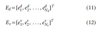
Huang et al¹¹ modeled the channel response as a two-dimensional image and used the super-resolution algorithm to recover the channel. Akiba et al¹² gave a channel estimation method dependent on deep learning, which employs a fully connected deep neural network (DNN) to jointly complete frequency domain interpolation besides estimation of frequency domain interpolation coefficients and uses LSTM cyclic neural network¹³ to jointly complete time domain state prediction as well as estimation of time domain correlation coefficients. The above method does not give too much consideration to the problem of adapting to the moving speed. When the moving speed and multipath conditions change, the distribution of channel data will fluctuate greatly. The performance of the above methods will decrease to varying degrees.

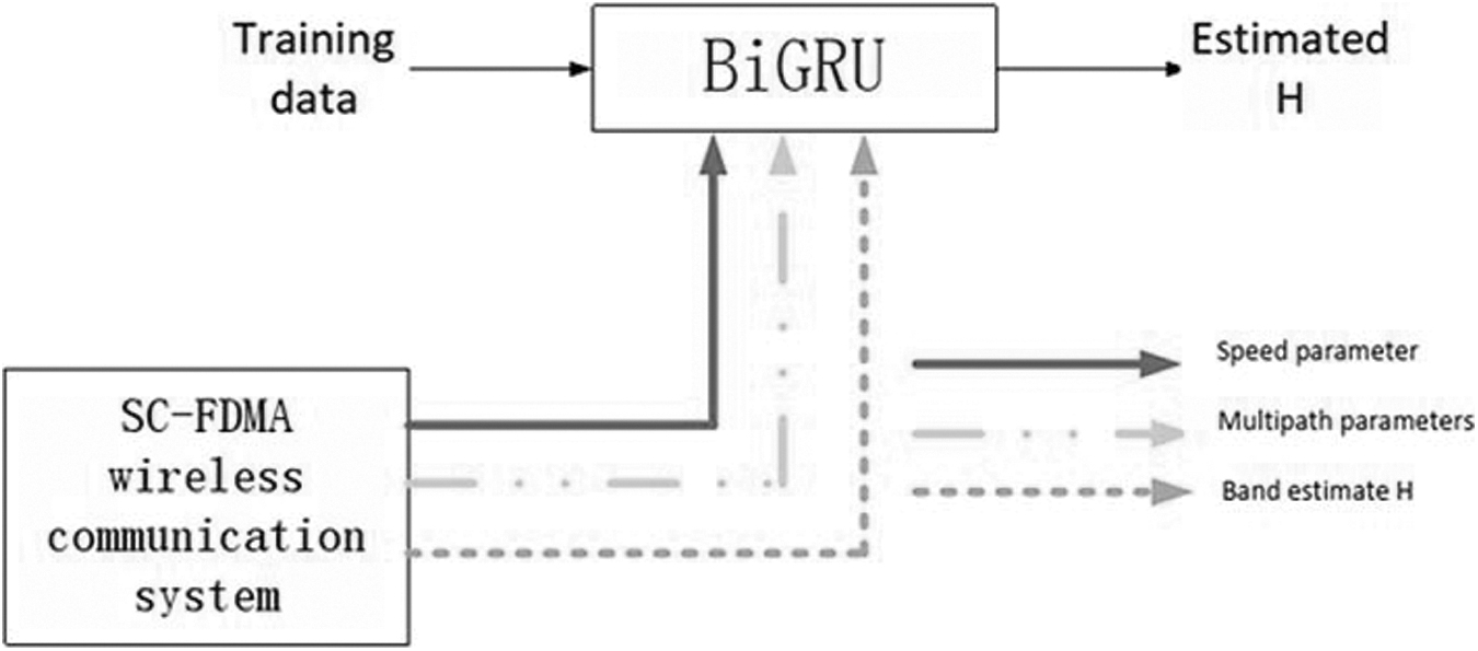
In response to the above problems, the channel estimation accuracy is further improved, thereby improving the communication quality of the 5G-V2X Internet of Vehicles. The 5G-V2X wireless communication scenario model is shown in Figure 1. In this article, the BEM¹⁴ is used as the intelligent channel estimation outline model. Then recommend a new high estimation algorithm for deep learning. The following are the particular components:

FIG. 1.

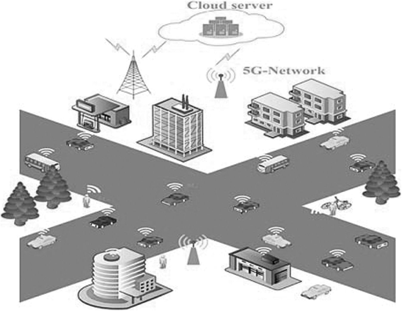
5G-V2X wireless communication scenario. V2X, vehicle-to-everything.

(1)

This article adopts the BEM of high-speed channel impulse response to build a simulation communication system based on SC-FDMA as the intelligent channel estimation framework for the Internet of Vehicles. The deep learning method is employed to complete the training of the channel estimation model.

(2)

Aiming at the problem that the performance of the estimation algorithm is greatly reduced due to the channel change in the high-speed mobile setting, this article introduces the multipath parameter as well as the speed parameter in the neural network. Then, a convolution module comprising multilayer convolution is designed to complete frequency domain interpolation. Gated recurrent unit¹⁵ (GRU) is used to design bidirectional gated recurrent unit (BiGRU) for time domain state prediction. The multipath code vector is applied to the output after multilayer convolution interpolation in the form of weighting, so as to track the change of channel multipath. BiGRU takes the speed vector as the input of the network and tracks the channel changes in different mobile environments through this vector. The program may acquire a priori multipath parameters by offline training, and velocity parameter vectors for different mobile scenarios, and can track channel changes in different mobile environments through these two parameters. So that correct channel data training may be achieved in a variety of mobile contexts, or the suggested algorithm's performance can be verified via modeling.

Related Works

SC-FDMA system transceiver signal processing

The 5G-V2X physical transmission system uses the SC-FDMA-based transmission mode.¹⁶ They will be able to connect with infrastructures, the internet, as well as every other according to V2X technologies. Smart automobiles can benefit from high-speed transmission, continuous networking capabilities, and compared to the results. It has the ability to deliver faster speeds, reduced delay, and more bandwidth than 4G long term evolution networks. It is among the globe's fastest and most accurate technology, which implies faster connections, less latency, and a big change as far as how we lived, collaborate, and perform. The baseband transmission model of the SC-FDMA system is shown in Figure 2. At the transmitting end, user data undergo discrete Fourier transform (DFT) precoding, subcarrier mapping, invert fast Fourier transform (IFFT), and cyclic prefix (CP) precoding. At the same time, the pilot generated by the Zadoff–Chu (ZC) sequence undergoes carrier mapping, IFFT, CP addition, and is transmitted to the space together with the user data.

FIG. 2.

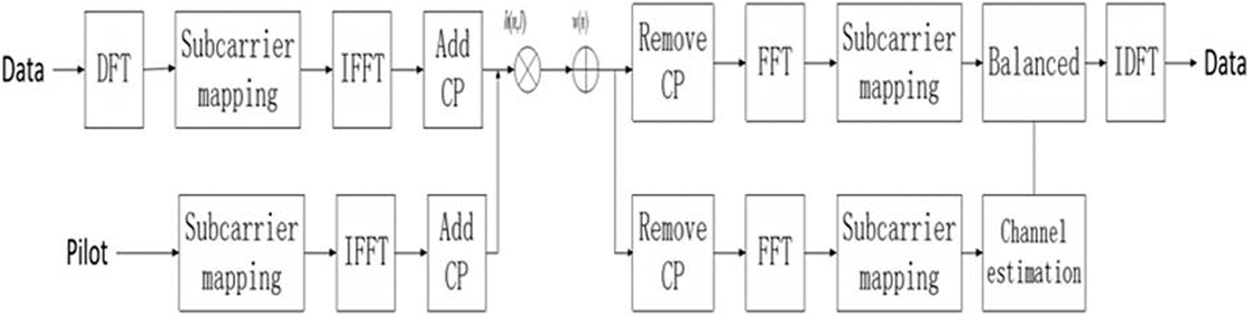
SC-FDMA baseband transmission model. CP, cyclic prefix; DFT, discrete Fourier transform; FFT, fast Fourier transformation; IDFT, inverse discrete Fourier transform; IFFT, invert fast Fourier transform; SC-FDMA, single-carrier frequency-division multiple access.

The inverse discrete Fourier transform (IDFT) method reverses the DFT procedure. It is also known as the reverse Fourier transform. It transforms a frequency domain signal from a space domain waveform. The allocation of data sequencing to different spectral elements produces the DFT signals. The DFT is a complicated measure of the rate that turns a limited succession of equitably observations of a functional into a same length series of equitably observations of the discrete time Fourier transform. The processing procedure of the receiving end is opposite to that of the transmitting end, and finally, the signal is resumed. Since the signal is affected by channel fading and noise, it is necessary to estimate the channel and use frequency domain equalization after fast Fourier transformation (FFT) to compensate for the influence caused by the channel to complete signal detection.

A transmission frame based on SC-FDMA in 5G-V2X contains I transmission symbols, including I_d data symbols and I_ppilot symbols, and the number of DFT points is M, and the total number of transmission subcarriers is N. Note that the i data symbol after modulation is and the transmitted data frequency domain symbol is obtained after M DFT transformation, and the ZC pilot sequence is inserted before the subcarrier mapping. A technique of configuring a hard drive in which the mechanical production removes the information of the disk through truncating them with zeros is known as zero filling.

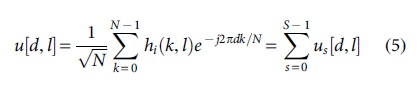
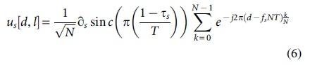
The term zero filling comes from the fact that every bit on the disk is substituted by a zero. The information can be retrieved from the storage device after it has been wiped with 0s. Accordingly, to complete the next N IFFT transformation besides moderate the frequency domain symbols to every subcarrier, the current frequency domain symbols need to be zero-filled, and the 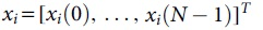$(N - M)$ subcarrier positions that are not transmitted as information need to be zero-filled to acquire the complete frequency. Transmit the symbol $X_{i} (k)$ in the domain and complete the IFFT operation to attain the transmit symbol in the time domain. Finally, add CP and perform digital-to-analog conversion as well as send it to the wireless transmission channel. Therefore, the SC-FDMA frequency domain transmission symbol can be expressed as: $X_{i} (k) = \{\begin{matrix} X_{i}^{d} (k), k \in k_{s i g n a l,} i = 0, 1, \dots, I_{d} - 1 \\ X_{i}^{p} (k), k \in k_{s i g n a l,} i = 0, 1, \dots, I_{p} - 1 \\ 0, k \in k_{z e r o,} i = 0, 1, \dots, I - 1 \end{matrix}$ (1)

Among them, $k_{s i g n a l}$ represents the information subcarrier, and $k_{z e r o}$ represents the zero-padded subcarrier.

After passing through the wireless channel of the Internet of Vehicles and successfully receiving at the receiving end, it is necessary to perform analog-to-digital conversion and de-CP operation and then perform FFT to obtain the frequency domain received symbol Y_i.

Design of the SC-FDMA system based on BEM

In the high-speed mobile environment, the channel has time-varying characteristics, and a DOPPLER FREQUENCY SHIFT owing to excessive motion will lead the frequencies mismatch of the SC-FDMA network subcarriers, which will lead to the destruction of the orthogonality between the SC-FDMA system subcarriers. This variation seriously affects the performance of the system. The conjugate transposition (or Hermitian transposition) of an m-by-n matrix A with complicated elements is the n-by-m matrix formed from A by obtaining the transposed and then the complicated conjugation of every column (the imaginary conjugation of a + ib is a − ib, for real values a or b).

It is commonly abbreviated as A^H or A*. Suppose that in the SC-FDMA system model, there are N subcarriers, and one subframe contains I SC-FDMA symbols. Suppose that the i subcarrier symbol on the n SC-FDMA symbol sent is 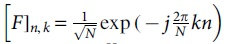$X_{i} (n), n \in [0, N - 1]$ , abbreviated as X_i. After X_i undergoes IFFT for SC-FDMA modulation, there is $x_{i} = F^{H} X_{i}$ , where x_i represents the transmitted time domain sequence, represents the Fourier matrix, and represents the conjugate transpose. The SC-FDMA broadcasting technique can be expressed as $y_{i} = h_{i} x_{i} + z_{i}$ .

Where 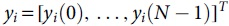is the time domain symbol vector received on the i-th SC-FDMA symbol; z_i is the complex additive white Gaussian noise; h_i is the channel impulse response matrix of the i-th SC-FDMA symbol, as demonstrated in the following formula: $h_{i} = [\begin{matrix} h_{i} (0, 0) & 0 & \dots & h_{i} (0, L - 1) & \dots & h_{i} (0, 1) \\ h_{i} (1, 1) & h_{i} (1, 0) & 0 & \dots & \dots & h_{i} (1, 2) \\ ⋮ & ⋮ & ⋮ & ⋮ & ⋮ & ⋮ \\ 0 & \dots & 0 & h_{i} (N - 1, L - 1) & \dots & h_{i} (N - 1, 0) \end{matrix}]$ (2)

Among them, $h_{i} (k, l)$ illustrates the channel impulse response of the l-th sampling point of the k-th tap within the i-th SC-FDMA symbol time. At the receiving end, the received symbol y_i in the time domain undergoes a FFT to obtain Y_i. $Y_{i} = F y_{i} = F h_{i} F^{H} X_{i} + F z_{i} = H_{i} X_{i} + Z_{i}$ (3)

H denotes the frequency domain response matrix of the i symbol, denoted as: $H_{i} = F h_{i} F^{H}$ (4)

The fast time-varying channel model is modeled as BEM, and the BEM function of the channel is obtained by the following formula:

Among them, $u_{s} [d, l]$ is defined as:

Among them, $l \in [0, L - 1]$ , $d \in [0, N - 1]$ , and $u_{s} [d, l]$ are single-tap BEM. $ϕ_{s} (l) = sin c (π (l - \frac{τ_{s}}{T}))$ (7)

Where $f_{s} N T$ is the normalized Doppler frequency shift.

In a general mobile communication system, the normalized Doppler frequency shift is much less than 1, that is, $|f_{s} N T| ≪ ≪ 1$ . The Doppler frequency shift throughout train travel may be estimated using the formula fd = v/c fc cos θ, where v is the vehicle velocity, c is the electromagnetic radiation rate, fc is the central sampling rate, and is the angular displacement between the transmitter as well as θ is the vehicle orientation. In high-speed mobile settings, the Doppler effect causes the electromagnetic transmitter reference signal (e.g., upstream f0, downstream f1) to change substantially.

Based on this feature, it can be reasonably assumed that each subcarrier only affects its adjacent D subcarriers, and then, the channel matrix H_i can be approximated as a band matrix, and the following formula is obtained after sorting: $H_{i} = [\begin{matrix} H_{0, 1} & \dots & H_{0, D - 1} \\ ⋮ & ⋱ & ⋱ \\ H_{D - 1, 0} & ⋱ & ⋱ \\ ⋱ & ⋱ & H_{N - D - 1, N - 1} \\ ⋱ & ⋱ & ⋮ \\ H_{N - 1, N - D - 1} & \dots & H_{N - 1, N - 1} \end{matrix}]$ (9)

The above formula retains the diagonal of H_i and the elements between the distance D on both sides of the diagonal, which greatly reduces the complexity of the model.

Methods

This section mainly introduces the channel estimation method using deep learning proposed in this article.

Channel prediction network structure using the deep learning method

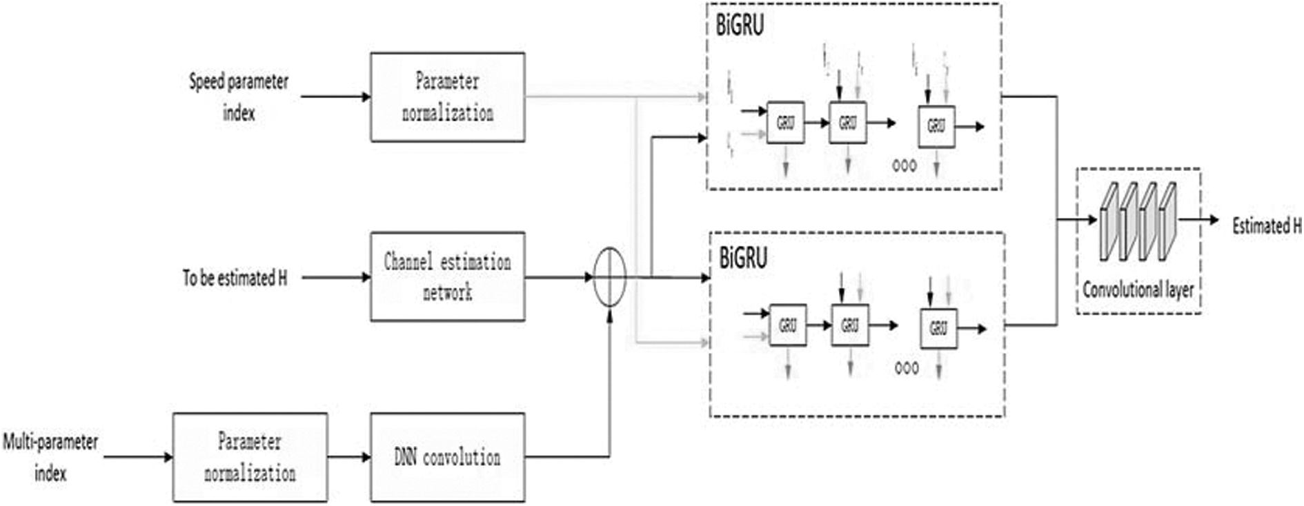
The overall channel estimation structure of this article is shown in Figure 3, which is mainly divided into two parts: training and prediction.

FIG. 3.

Channel prediction network framework. BiGRU, bidirectional gated recurrent unit.

We train the channel prediction network and get the parameters of the network through training. Through multiple training iterations, the optimal solution of the loss function of the algorithm is solved, so as to learn the change characteristics of the channel. Due to the general hidden layers, neural nets are stronger at data modeling. To create forecasts, statistical models simply utilize transmitter and receiver vertices. The hidden state is also used by the neural network to improve forecasting accuracy. This is because it “learns” in the same manner that humans do. In the prediction stage, through the trained network parameters, the channel prediction network can be used to continue to track and predict the real-time complete live channel estimate with channel modifications.^17–19

The technique of detecting association among the understanding of the various values on the left as well as the matrix of arithmetic operations on the right is known as channel estimation. The technique of estimation used in particular might vary based on the execution. The channel estimation network is composed of a multilayer convolutional neural network and a GRU module. In a deep CNN, the convolutional layer processes the original image in several ways. In this system, it refers to the common way of convolutional processing.

The quantity of granules as well as the shape of the particles are by far the most critical characteristics. The multiple levels are 1 × 1, 3 × 3, and 1 × 1 fully connected layers, with the 1 × 1 layer lowering and then raising (preserving) proportions, as well as the 3 × 3 layer acting as a bottleneck with reduced input/output measurements. The specific structure is shown in Figure 4. Among them, multilayer convolution includes 1 × 1 convolution and 3 × 3 convolution. The specific structure is shown in Figure 5.

FIG. 4.

Channel prediction network.

FIG. 5.

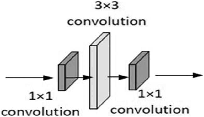
Multilayer convolution structure.

Channel prediction network model

The channel prediction network includes data preprocessing, multivector parameter process, and frequency domain interpolation starts with channel prediction and data dimensionality reduction.

Data preprocessing part

Channel estimation is to evaluate the channel frequency domain response matrix H at the receiving end. In the pilot-based channel estimation technology, the main goal is to forecast the data symbol channel response based on the pilot symbol channel response. By using least squares approach, an investigator will create a line of greatest fit that illustrates the possible link among two or more variables. The linear regression approach explains why the line of greatest fit should be placed among some of the information items under consideration. The input of the channel prediction network model is a subframe size conditional random field matrix, and the channel response at the position of the LS technique is used to initialize the pilot symbol in the matrix. The channel response value at the data symbol position is set to zero. It can be expressed by the following formula:

Among them, 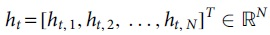is at the data symbol position $h_{t, n} = 0$ . Because the original channel response information is difficult, it is essential to preprocess the information prior inputting the channel prediction model. In this article, we excerpt the real as well as imaginary parts of the source channel information and then concatenate them into single dimension. The channel data become $H' = ℛ^{T \times 2 N}$ , $h' = ℛ^{T \times 2 N}$ .

Multiparameter process

To overcome the influence of the mobile environment on channel estimation, we introduce multipath parameters and speed parameters in frequency domain interpolation besides time domain state prediction, respectively. The word interpolation relates to the procedure of transforming a recorded transmitted data (including a sampling speech signals) to one of a greater samples per second (upsampling) utilizing modern multimedia modulation technique in the realm of digital signal analysis (convolution with such a frequency-limited impulsive input for illustration).

Interpolating a succession of time domain sampling is a common (and essential) digital signal processing operation, as well as there are several explanations of time domain extrapolation (a type of template matching) in the research as well as on the internet. These two parameters are used to track changes in multipath conditions and changes in moving speed in a connected car environment. We use the normalization method in deep learning to convert the above two parameters into a vector of the same latitude through a normalization operation. The normalization operation uses a fully connected network, and the output is correspondent toward the weight in the fully connected network. We named the multipath parameter and speed parameter as N_d and N_v, respectively, and the output dimension is $2 N$ . Then, the normalized matrix can be illustrated as:

Among them, $E_{d} \in ℛ^{N_{d} \times 2 N}$ and $E_{v} \in ℛ^{N_{v} \times 2 N}$ . The information in the embedding matrix is stochastic in the learning process. During training, we only need to give the index $v_{i n d e x}$ and $d_{i n d e x}$ corresponding to each speed and multipath of the embedding layer. The embedding layer uses the supplied index to get the provided sequence in the embedding matrices as the eventual output sequence.

Multi-convolution frequency domain interpolation

Compared with other methods²⁰ using complex DNN for frequency domain interpolation, the interpolation of each SC-FDMA symbol is relatively independent. As a result, the frequency domain interpolation does not make good use of the time domain change characteristics of the channel. Therefore, we use a simple multi-convolution operation for frequency domain interpolation. This module further utilizes the information of the input convolution kernel size on every channel to perform feature extraction and data sorting on the data through two 1 × 1 and one 3 × 3 convolutions. This method can simultaneously utilize the change characteristics of the channel in the time domain and the frequency domain.

Let $L_{k - 1} = [l_{k - 1}^{1}, l_{k - 1}^{2}, \dots, l_{k - 1}^{C_{k - 1}}] \in ℛ^{H_{k - 1} \times C_{k - 1}}$ be the outcome of the $k - 1$ -th layer of the multi-convolution module, where $l_{k - 1}^{c} \in ℛ^{H_{i - 1}}$ illustrates the data vector on the c-th channel. So, the ith result on the c-th channel on the k-th layer of convolutional neural network is:

c = 1, 2, \dots, C_{k}

(13)

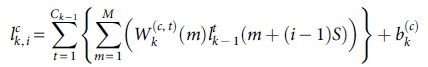
Among them, $W_{k} \in ℛ^{C_{k - 1} \times C_{k} \times M}$ and $b_{k} \in ℛ^{C_{k}}$ , respectively, represent the weight tensor as well as bias vector of the first layer, S is the step length of the convolution filter sliding on the input information, and M is the width of the convolution filter. C_k represents the number of channels output by the k-th convolutional neural network. Hence, we can get the resultant vector on the c-th channel on the k-th convolution as:

The resultant data of layer k are as follows: $l_{k} = [l_{k}^{1}, l_{k}^{2}, \dots, l_{k}^{c_{k}}] \in ℛ^{\frac{H_{k - 1} - M + 1}{S} \times C_{k}}$ (15)

Essentially stated, an activation function can be defined that is applied to an artificial neural network to aid it in learning complicated trends in information. As compared toward a neuron-based paradigm seen in human minds, the training algorithm is responsible for determining whatever is to be discharged toward the next neurons at the conclusion of the process. Each layer of convolutional network is followed by an activation function, so the transformation formula of every layer can be simplified as: $L_{k} = f ({W_{k}}^{*} L_{k - 1} + b_{k})$ (16)

The number of input besides output channels of the channel prediction network is T. Then, the channel response on the n-th subcarrier on the t-th SC-FDMA symbol is as follows:

t = 1, \dots, T; n = 1, \dots, N

(17)

Among them, $W \in ℛ^{2 N \times 2 N}$ —weight matrix of the multipath code vector. Since the convolutional neural network's structural change reduces the complexity of the source information, we will set padding = 1 when inputting. Add 0 during convolution to ensure that the output is consistent with the original input dimension. When estimating the channel frequency domain response on the n-th subcarrier on the t-th SC-FDMA symbol, not only the channel frequency domain response at the pilot symbol is closer to the nth subcarrier at the SC-FDMA symbol but also other SC-FDMA symbols are used. The frequency domain response of the channel at the pilot symbol is closer to the nth subcarrier at the FDMA symbol.

Therefore, the frequency domain interpolation method proposed in this article jointly utilizes the time/frequency domain change relationship of the channel, and at the same time tracks the time/frequency domain change of the channel frequency domain response. The frequency domain reaction of the channels at the piloted signal as well as the multipath coding vectors define the channel estimation at every transmission symbolism. The multipath vectors are employed to monitor environmental changes induced through variations in the channel's multipath circumstances. The outcome next to interpolation for every SC-FDMA symbol can be illustrated as: $h_{t}^{''} = f_{T} (W^{(t)} * H' + W_{d} c_{d})$ $t = 1, 2, \dots, T$ (18)

Among them, t corresponds to the number of output channels in the multi-convolution module.

GRU time domain state prediction

To be able to correct to the mobile environment, we use the GRU network when predicting the time domain state. The network converts various movement velocities into a matrix, which it then feeds into the time domain information system. The network introduces two specific inputs: the speed parameter in the mobile environment as well as the channel information after frequency domain interpolation. We added newly introduced parameters to the loop structure of the original GRU network. The overall structure is shown in Figure 6.

FIG. 6.

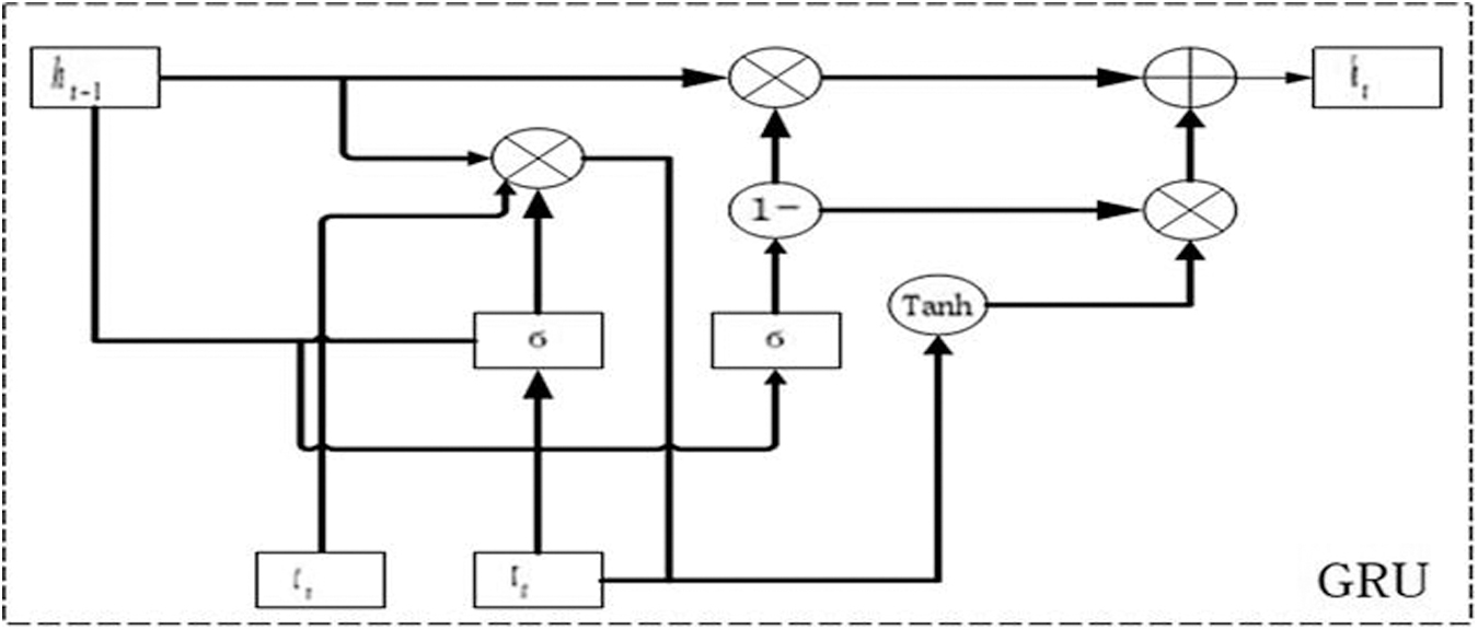
Schematic diagram of GRU network structure. GRU, gated recurrent unit.

The GRU system is mostly made up of GRU divisions. Every gate control device has two gates: an input gateway and an updated gateway. The information intake in every component of the system is controlled by the input nodes and updating gates. From this, we can obtain the time domain state forecasting mathematical transformation formula for the t-th SC-FDMA symbol: $i_{t} = σ (W_{i} [h_{t}^{''}, h_{t - 1}^{'''}])$ (19) $u_{t} = σ (W_{u} [h_{t}^{''}, h_{t - 1}^{'''}])$ (20)

c_{t} = tanh (W_{c} [U_{t} ⨀ h_{t}^{''}, h_{t - 1}^{''}] + i_{t} ⨀ V_{c} c_{v})

(21)

h_{t}^{''} = u_{t} ⨀ c_{t} + (1 - u_{t}) ⨀ h_{t - 1}^{''}

(22)

Where i_t and u_t are the input gate and update gate of the gated recurrent unit (GRU), respectively; c_t is the memory unit, where σ is the Sigmoid function; is the channel data input at time t; is the state of the previous GRU unit at time $t - 1$ ; U_i, W_i, U_u, W_u, U_c, W_c, V_c are weights of the network obtained by the GRU through training; $⨀$ is the element multiplication; and c_v is the code vector at a specific speed.

We apply the input gate to the speed parameter part. This is intended to control the flow of only a portion of the information from the speed code into the memory cell in the form of a gate. It is possible that the information in the memory cell will not be completely controlled by the speed code, but rather a fusion of various information. Finally, the memory cell and input are directly controlled through an update gate to attain the final output. Underneath low-speed conditions, in the temporal domain, the network response varies gradually, so the value of u_t is small, and then, the last outcome is mainly determined by the input. The sampling frequency of the received signals, however, displays fast time-varying features in this time under high-speed movement situations. The value u_t is large, so the final output is determined by the memory unit that contains the influence of the Doppler frequency shift parameter.

We refer to the design of two-way LSTM and adopt a two-way GRU (BiGRU) network.^21–23 GRU is a multilayer perceptron that seeks to tackle the overfitting issue. Since both are constructed identically and, in certain situations, achieve comparably outstanding outcomes, GRU might be regarded as a variant of the LSTM. This system is made up of two GRU systems, one that does upward forecasting and the other that does backward forecasting. For the forecast of the present moment, this may make effective utilization of any data during the specific moment. Bidirectional forecasting can prevent experimental error produced by unidirectional predictive model. Every GRU network has T number of GRU units. The results of the two GRUs at time t in the BiGRU network are as follows:²⁴ $h_{F W, t} = G R U (h_{F W, t - 1}, h_{t}^{''}, c_{v}, Θ_{F W})$ (23)

h_{B W, t} = G R U (h_{B W, t - 1}, h_{T - t + 1}^{''}, c_{v}, Θ_{B W})

(24)

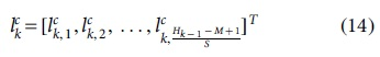
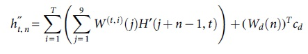
Among them, $Θ_{F W}$ (forward [FW]) and $Θ_{B W}$ (backward [BW]) are all parameters in the forward GRU and subsequent GRU networks, respectively. So, the output of the BiGRU network at time t is: $h_{t}^{''} = [h_{F W, t}; h_{B W, t}] \in ℛ^{4 N \times 1}$ (25)

The final prediction result is that the output at each moment is the concatenation of the two GRU outputs; the final result is dimensionally reduced (DR) to unify the data to the same dimension. The final channel estimation result of the SC-FDMA symbol at time T is as follows:²⁶ $ĥ_{t} = f_{T} (W_{D R} h_{t}^{'''})$ (26)

Experimental Results and Analysis

Model training settings

We use the BEM channel model to generate training data. The collection of training samples in offline learning is accomplished by collecting data set from all resource's panels in every frame via simulation environment and then setting the received signal at the information to 0 using particular pilot insertion criteria. The index value of each sample corresponding to speed and multipath is used as training data. The channel estimation network is trained through the training data to obtain the minimized loss function. The parameters of the channel estimation network are as follows: time domain correlation coefficients, frequency domain interpolation coefficients, parameter embedding matrix, as well as dimensionality reduction coefficients. Through training, the parameters in the network can better track changes in the channel.

In required to practice the channel estimation network, assume the transforming equation and therefore entire variables of the whole channel estimation network are 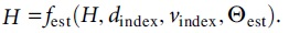$f_{e s t} ()$ and $Θ_{e s t}$ , respectively, so the channel state information obtained by the channel estimation network can be expressed as Gradient descent is an optimal scheduling approach for determining a function's local optimal. To use gradient descent to discover a method's single value, we must take measures proportionate toward the negativity of the stored procedure gradients (shift away from the gradients) at the present location. The gradient descent method uses the momentum-driven stochastic gradient descent method. This method can adjust learning parameters through appropriate momentum and can well balance training speed and training results. Our loss function is defined as:

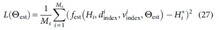
Among them, $H^{*}$ is the supervised data, and M_s is the total number of samples in the training sample set.

The training set, verification set besides test set we use are, respectively, 300,000, 40,000 and 20,000. The various data sets contain the channel data to be evaluated, and then, the index value $v_{i n d e x}$ and multipath index value $d_{i n d e x}$ correspond to the speed of each data sample. The moving velocity factor set of the channel data contained in various data sets is [50, 150, 200 km/h], namely $v_{i n d e x} = [0, 1, \dots, 5]$ , then the multipath number set is [3, 6, 9, 12, 15], namely $v_{i n d e x} = [0, 1, \dots, 5]$ .

Model complexity analysis

First, we compared the complexity of the BEM channel model and the traditional channel model, and the comparison results are shown in Table 1. We mainly compared the number of multiplication operations and time complexity of the algorithm.

Table 1.

Comparison of the Complexity of the Basic Expansion Model Channel and the Traditional Channel Model

Channel estimation algorithm	No. of multiplication operations	Time complexity
LS²⁵	$4 N$	$o (N)$
LMMSE²⁶	$3 N^{3} + N^{2}$	$o (N^{3})$
BEM

BEM, basic expansion model; LMMSE, linear minimum mean square error; LS, least square.

It can be seen from Table 1 that the LS algorithm has the lowest complexity, which is linear order; the LMMSE algorithm has the highest complexity. Since N >> DL, the complexity of the BEM-LS algorithm is much lower than that of the LMMSE algorithm. Compared with the LS algorithm, the complexity of the BEM algorithm is relatively higher, but the higher part is not much, and the result is better than the former. Therefore, the complexity of the BEM algorithm we used is within the tolerable range of research.

Finally, we analyzed the computational complexity of the four traditional channel estimation methods, LS, LMMSE, spectral time average (STA), and constructed data pilots (CDP), the DNN-LSTM algorithm, and the algorithm proposed in this article. This article mainly compares the algorithm to estimate the number of multiplications and computational complexity required for two SC-FDMA symbols. One SCFDM symbol contains pilots, besides the other SC-FDMA symbol adjacent to it does not contain pilots. Table 2 depicts the outcome of analyzed complexity of anomaly techniques.

Table 2.

Comparison of the Complexity of Different Algorithms

Channel estimation algorithm	No. of multiplication operations	Time complexity
STA	$[N] + [2 N]$	$o (N)$
CDP	$[N] + [4 N]$	$o (N)$
LMMSE+Linear interpolation	$[3 N^{3} + N^{2}] + [N]$	$o (N^{3})$
LS+Linear interpolation	$[N] + [N]$	$o (N)$
OURS	$[(2 M T + 2 N_{d}) N] + [64 N^{2} + (2 N_{v} + 12) N]$	$o (N^{2})$

CDP, constructed data pilots; STA, spectral time average.

The convergence speeds of LS, STA, and CDP are all in the identical magnitudes, as shown in Table 2. Owing to the necessity to perform transformation function, LMMSE has the greatest overhead of the algorithm. The DNN-LSTM approach has a similar online estimate difficulty toward the spectrum sensing networks in this research, which is fewer than the minimum LMMSE with linear programming method and somewhat greater compared with the LS with linear interpolation technique. The channel estimation network is only the multiplication and addition of some matrices, so its complexity is lower than that of the traditional LMMSE algorithm.

In addition, the neural network can run in parallel, so the calculation time of the algorithm can be reduced. The training parameters are immediately used toward the channel estimation during the live assessment step; hence, the complication is modest. Even though the channel coding networks has the same model complexity as the DNN-LSTM technique, the quantity of arithmetic operations needed indicates that the beamforming system has a lower performance than the DNN-LSTM technique. In general, the complexity of our proposed method is within an acceptable range; it can be better used in complex car networking environments.

Simulation result analysis

In the simulation experiment, the channel model adopts the BEM. A subframe in the transmission system contains 14 transmission symbols, of which the 3rd, 6th, 9th, and 12th symbols are pilot symbols, and the rest of the system parameter settings are shown in Table 3.

Table 3.

Channel Parameter Setting

Channel estimation algorithm	No. of multiplication operations
Carrier frequency	5.9 GHz
Channel bandwidth	10 MHz
No. of carrier waves	500
Channel model	BEM
No. of channel taps	[3, 6, 9, 12, 15]
Maximum relative speed	[50, 150, 200] km/h

First, we simulated the effectiveness of the BEM by setting different relative moving speeds of the vehicle terminal (150 km/h for medium speed, and 300 km/h for high speed) and related to the existing LS technique. For comparison, the simulation indicators include the normalized mean square error (NMSE) and bit error rate (BER).

Figure 7 analyzes the NMSE and BER efficiency of the LS technique than the LMMSE algorithm in medium-speed and high-speed environments. It can be seen that in the medium-speed environment, although the LMMSE algorithm considers the influence of noise, since the channel impulse response changes within one symbol in the high-speed mobile environment, neither the LMMSE algorithm nor the LS algorithm can capture the change.

FIG. 7.

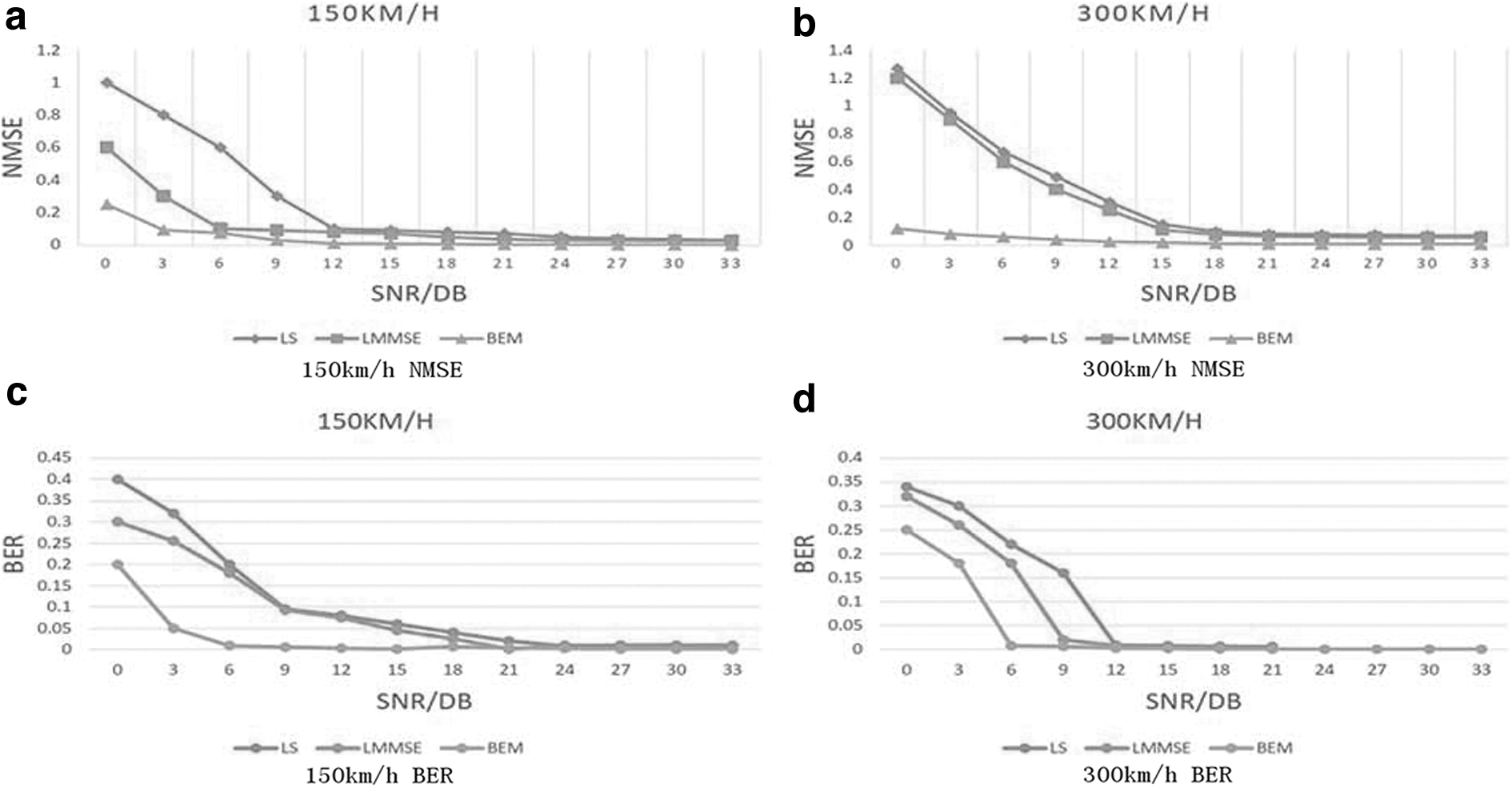
Comparison of the BER and NMSE algorithms for various channel estimation algorithms. BER, bit error rate; NMSE, normalized mean square error; SNR, signal-to-noise ratio.

Therefore, the performance gap between the two has narrowed. The BEM algorithm uses a base extension model to capture changes, so the performance is much better compared with the LS as well as LMMSE methodologies. In a high-speed environment, the advantages of the LMMSE algorithm over the LS algorithm are further reduced, and the LMMSE algorithm has little advantage and high complexity. And BEM can continue to maintain its advantage, still maintaining 5 dB of NMSE gain and 2 dB of BER gain. In summary, we use the BEM algorithm to be more suitable for the high-speed mobile car networking environment.

After that, we compared experiments with different multipath numbers and speeds. Figure 8 shows the NMSE as well as BER accomplishment of several techniques when the multipath number is 9 and the moving speed is 150 km/h. CDP, LS+linear interpolation besides STA algorithms all exhibit poor NMSE efficacy, as shown in the figure. This is because the channel responses at the pilots of these algorithms are all estimated by the LS algorithm, and then, the LS algorithm is incapable of removing noise's impact. This has an effect on the achievement of the information symbols stream responsiveness prediction. LMMSE has good NMSE performance, and the channel estimation network algorithm in this article has the best NMSE performance, which shows that the channel estimation algorithm in this article can not only effectively eradicate the influence of noise at the pilot frequency but also can better monitor the variations of the channel.

FIG. 8.

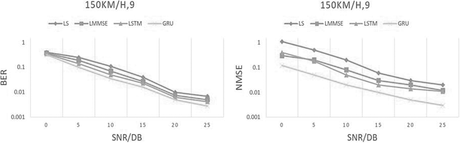
Performance comparison of the BER and NMSE of this algorithm when the number of multipath is 9 and the moving speed is 150 km/h. LMMSE, linear minimum mean square error; LS, least square; LSTM, long-term short memory.

For the DNN-LSTM algorithm, since the training data contain channel data of various environments, it cannot fit the channel data of different environments, so the performance is poor. At the time of the signal-to-noise ratio (SNR) <20, the BER efficiency of the DNN-LSTM technique is equivalent to the LMMSE performance. This shows that the neural network-based solution performs better in terms of noise removal as well as noise resilience. At this time, this article channel estimation method has attained the upper limit of estimation accomplishment. The impact of noise is now limiting the BER effectiveness of this approach.

Figure 9 shows the assessment of the NMSE and BER efficacy of various algorithms with multipath variations at the time of SNR = 25 dB and the moving speed is 150 km/h. The NMSE besides BER efficiency of several methodologies illustrate a downward trend as the moving speed enhances. The NMSE and BER efficiency of the STA, CDP, LS, besides LMMSE algorithms of STA, CDP, LS, and LMMSE decline sharply, representing that the existing technique is less robust to multipath. At this time, the decline trend of the CNN-GRU algorithm is relatively steady, signifying that the proposed method has much robustness.

FIG. 9.

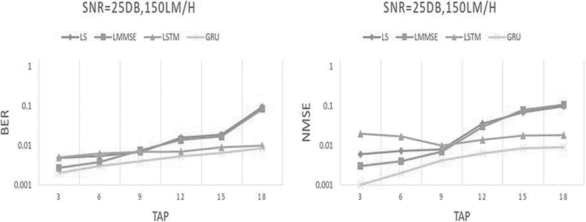
Performance comparison of the BER and NMSE of different algorithms when the moving speed is 150 km/h and SNR = 25 dB.

At this time, the NMSE performance curve of the DNN-LSTM technology fences with the variation of the multipath number, that is, the DNN-LSTM algorithm cannot efficiently monitor the changes in the channel multipath conditions, and the channel estimation algorithm in this article introduces multipath coding. The vector can accurately track the change of each multipath condition, which improves the algorithm's robustness to multipath.

Conclusions

To further enhance the quality of V2I communication in the Internet of Vehicles, this article first established a BEM channel model based on the sparse features of high-speed mobile channels. Dependent on the constructed BEM, a 5G-V2X-based intelligent channel estimation model is designed. Aiming at the problem of insufficient efficiency of existing channel estimation in the Internet of Vehicles environment, a channel estimation network based on deep learning is proposed, which uses multilayer convolution to complete frequency domain interpolation, as well as BiGRU for time domain state prediction, which enhances the accurateness of channel estimation.

To accomplish exact learning, we incorporate movement parameters matrix and multipath variable matrix as additional information to regulate the outcome of the complete spectrum sensing networks. Analysis as well as system simulation illustrate that the intelligent channel estimation model proposed in this article can ensure the accuracy and robustness of channel estimation while reducing complexity.

Footnotes

Authors' Contributions

J.H.: Writing—original draft (lead), data curation, software (lead), editing (equal). C.X.: Conceptualization (lead), methodology (lead), writing—original draft (lead), formal analysis (lead), writing—review and editing (equal). Z.J. and S.X.: Writing—review and editing (equal). T.L.: Conceptualization (supporting), writing—original draft (supporting). N.M.: Conceptualization (supporting). Q.Z.: Writing—original draft (supporting).

Data Sharing Agreement

The data sets used and/or analyzed during the current study are available from the corresponding author on reasonable request.

Author Disclosure Statement

No competing financial interests exist.

Funding Information

This article is a general project of science and technology plan of Beijing Municipal Education Commission (KM202110857002), the key project of Beijing Information Technology College (XY-YN-07-201902), the National Natural Science Foundation of China (Grant No. 62102033, 62171042).

Abbreviations Used

References

Wang

, Wang

, Cui

, et al. Survey on cooperatively V2X downloading for intelligent transport systems. IET Intell Transp Syst, 2019; 13(1):13–21.

Yuan

, Wang

, Xu

, et al. Multi-vehicle group-aware data protection model based on differential privacy for autonomous sensor networks. IET Circuits Devices Syst, 2022; 1–13.

Hassan

, Baig

, Asif

. Key technologies for ultra-reliable and low-latency communication in 6G. IEEE Commun Stand Mag, 2021; 5(2):106–113.

Hakeem S A

, Hady A

, Kim H

. 5G-V2X: Standardization, architecture, use cases, network-slicing, and edge-computing. Wirel Netw, 2020; 26(8):6015–6041.

Bhattacharya

, Tanwar

, Bodkhe

, et al. EVBlocks: A blockchain-based secure energy trading scheme for electric vehicles underlying 5G-V2X ecosystems. Wirel Pers Commun, 2021:1–41.

Sharma

, You

, Guizani

. Security of 5G-V2X: Technologies, standardization, and research directions. IEEE Netw, 2020; 34(5):306–314.

Bagheri

, Noor-A-Rahim

, Liu

, et al. 5G NR-V2X: Toward connected and cooperative autonomous driving. IEEE Commun Stand Mag, 2021; 5(1):48–54.

, Wu

, Liu

, et al. Blockchain-oriented privacy protection of sensitive data in the internet of vehicles. IEEE Trans Intell Vehicles, 2022:1–13.

Liao

, Cai

, Sun

, et al. Deep learning channel estimation based on edge intelligence for NR-V2I. IEEE Trans Intell Transp Syst, 2021; 23(8):13306–13315.

10.

Huang

, Zhang

, Gao

, et al. MIMO radar aided mmWave time-varying channel estimation in MU-MIMO V2X communications. IEEE Trans Wirel Commun, 2021; 20(11):7581–7594.

11.

Huang

, Xu

, Ji

, et al. AFLPC: An asynchronous federated learning privacy-preserving computing model applied to 5G-V2X. Secur Commun Netw, 2022; 2022: 1–11.

12.

Akiba

, Ishihara

, Sugiura

. Variable-block-length joint channel estimation and data detection for spatial modulation over time-varying channels. IEEE Trans Veh Technol, 2020; 69(11):13964–13969.

13.

X L

, GIANNAKIS G

, OHNO

. Optimal training for block transmissions over doubly selective wireless fading channels. IEEE Trans Signal Process, 2003; 51(5):1351–1366.

14.

Ahmed

, Nie

, Chen

, et al. DFT-spread OFDM with quadrature index modulation for practical VLC systems. Opt Express, 2021; 29(21):33027–33036.

15.

, Mitra

Improved atomic norm based time-varying multipath channel estimation. IEEE Trans Commun, 2021.

16.

ZUO

H L

, SONG H G

, AN T

, et al. Channel modeling and estimation in high-speed mobile environment. In: 2016 IEEE 83rd Vehicular Technology Conference. IEEE Press: Piscataway; 2016; pp. 1–5.

17.

Sak

, Senior A

, Beaufays

. Long short-term memory recurrent neural network architectures for large scale acoustic modeling. Interspeech, 2014; 338–342.

18.

, Lin

, Alazab

, et al. Deep learning-based traffic safety solution for a mixture of autonomous and manual vehicles in a 5G-enabled intelligent transportation system. IEEE Trans Intell Transp Syst, 2020; 22(7):4337–4347.

19.

Giannakis

G B

, Tepedelenlioglu

. Basis expansion models and diversity techniques for blind identification and equalization of time-varying channels. Proc IEEE, 1998; 86(10):1969–1986.

20.

Pan

, Shan

, Li

, et al. Channel estimation based on deep learning in vehicle-to-everything environments. IEEE Commun Lett, 2021; 25(6):1891–1895.

21.

Chung

, Gulcehre

, Cho K

, et al. Empirical evaluation of gated recurrent neural networks on sequence modeling. arXiv preprint arXiv:1412.3555 2014.

22.

Mantri

, Prasad

. Mobility and heterogeneity aware cluster-based data aggregation for wireless sensor network. Wirel Pers Commun, 2016; 86(2):975–993.

23.

Nair

, Pillai

. A new approach for improving performance of localized SC-FDMA LTE

Uplink

. In: 2021. 2nd International Conference on Advances in Computing, Communication, Embedded and Secure Systems (ACCESS). Ernakulam, India: IEEE; 2021; pp. 18–23.

24.

Wan

, Fang

, Duan

, et al. Generalized Bussgang LMMSE channel estimation for one-bit massive MIMO systems. IEEE Trans Wirel Commun, 2020; 19(6):4234–4246.

25.

Soltani

, Pourahmadi

, Mirzaei

, et al. Deep learning-based channel estimation. IEEE Commun Lett, 2019; 23(4):652–655.

26.

Liao

, Hua

, Dai

, et al. ChanEstNet: A deep learning based channel estimation for high-speed scenarios. In: 2019–2019 IEEE International Conference on Communications (ICC). Shanghai, China: IEEE; 2019; pp. 1–6.