
Abstract
Resting state functional connectivity reveals intrinsic, spontaneous networks that elucidate the functional architecture of the human brain. However, valid statistical analysis used to identify such networks must address sources of noise in order to avoid possible confounds such as spurious correlations based on non-neuronal sources. We have developed a functional connectivity toolbox Conn (
Introduction
F
Low-frequency resting state networks (<0.1 Hz) reveal coherent, spontaneous fluctuations that delineate the functional architecture of the human brain (Biswal et al., 1995, 2010; Buckner et al., 2008; Fox et al., 2005; Fox and Raichle, 2007). Such networks were initially discovered for the motor system (Biswal et al., 1995), but have also been discovered for both task-positive and task-negative (i.e., default, Raichle et al., 2001) neural systems (Fox et al., 2005; Fransson, 2005; Kelly et al., 2008; Uddin et al., 2009). Resting state networks have been shown to be robust and reliable (Chen et al., 2008; Damoiseaux et al., 2006; Shehzad et al., 2009; Zuo et al., 2010a, 2010b), and to exist in infants (Fransson et al., 2007), during sleep (Fukunaga et al., 2006; Horovitz et al., 2008), under light sedation (Greicius et al., 2008) and under anesthesia in primates (Vincent et al., 2007). Such networks have been associated with individual differences in healthy people (Mennes et al., 2010). Because rest has no behavioral demands, resting state connectivity is particularly useful for characterizing functional brain network differences in pediatric and clinical populations, such as schizophrenia (Whitfield-Gabrieli et al., 2009; Whitfield-Gabrieli and Ford 2012), ADHD (Castellanos et al., 2008), autism (Weng et al., 2010), depression (Greicius et al., 2007; Hamilton et al., 2011), bipolar disorder (Chai et al., 2012), and Alzheimer's disease (Buckner et al., 2009; Greicius et al., 2004; Wang et al., 2007).
The two most common analytical approaches toward analyzing resting state functional connectivity (RSFC) data are ICA (e.g., Beckmann et al., 2005, 2009; Greicius et al., 2007; Stevens et al., 2009) and seed-driven RSFC (e.g., Biswal et al., 1995; Castellanos et al., 2008; Greicius et al., 2003; Fox et al., 2005). In seed-driven RSFC analysis, Pearson's correlation coefficients are calculated between the seed time course and the time course of all other voxels, after which correlation coefficients are typically converted to normally distributed scores using Fisher's transform to allow for second-level General Linear Model analysis. Correlation maps often depend on the specific location of the seed, so that seed-driven RSFC has been used to dissociate functionally and anatomically heterogeneous regions of interest (Di Martino et al., 2008; Margulies et al., 2007; Roy et al., 2009; Uddin et al., 2010), and to delineate functional topography in the brain by sharp transitions in correlation patterns that signal functional boundaries across cortex (Cohen et al., 2008).
In functional connectivity analysis, it is critical to appropriately address noise in order to avoid possible confounding effects (spurious correlations based on non-neuronal sources). Standard methods dealing with blood oxygen level-dependent (BOLD) contrast signal noise sources that may be appropriate in the context of the estimation of task- or condition-dependent BOLD signal responses (e.g., regression of subject movement parameters in standard functional analysis) may not suffice in the context of the estimation of functional connectivity measures. For activation studies, the risk of only partially removing BOLD signal noise sources is typically a potential decrease of sensitivity (increasing type II errors), whereas for resting connectivity studies, the risk is a potential decrease of validity (increasing type I errors). Therefore, a more conservative approach to controlling the effects of BOLD signal noise sources is warranted in the context of functional connectivity analysis compared with that of standard functional analysis. In Chai et al. (2012) we showed how a method for reducing spurious sources of variance in BOLD and perfusion-based fMRI, the anatomical component-based noise correction method (aCompCor) (Behzadi et al., 2007), can be particularly useful in the context of fcMRI analysis, increasing not only the validity, but also the sensitivity and specificity of these analyses. Compared to methods that subtract global signals from noise regions of interest (ROIs), the CompCor method is more flexible in its characterization of noise. It models the influence of noise as a voxel-specific linear combination of multiple empirically estimated noise sources, which are estimated from the variability in BOLD responses within noise ROIs. This is particularly appropriate for fMRI noise sources as cardiac and respiratory effects do not have a common spatial distribution in their effects (e.g., cardiac effects are particularly visible near vessels and respiratory effects appear more globally and stronger near edges in the image). Removal of this richer characterization of the range of voxel-specific noise effects and additional movement and possible task-related covariates, together with temporal filtering and windowing of the resulting BOLD signal at each voxel, provides increased protection against possible confounding effects in RSFC without introducing artifactual biases in the estimated connectivity measures.
In addition to physiological artifacts, head motion artifacts have been shown to significantly influence intrinsic functional connectivity measurements (Satterthwaite et al., 2012; Van Dijk et al., 2012). Moreover, it has been recently demonstrated that artifacts in the functional time series may result in substantial changes in RSFC data despite standard compensatory regression of motion estimates from the data (Power et al., 2012). These findings suggest that rigorous artifact rejection in addition to motion regression is especially prudent for valid interpretation of RSFC. Conn is seamlessly interoperable with quality assurance and artifact rejection software, art (
With the increase in popularity of linear functional connectivity analysis, there is still a large degree of variability in the exact methods used for the analysis of fcMRI data, with differences in noise-preprocessing steps as well as differences in the characterization of fcMRI measures across labs, which can complicate the interpretation and comparison of fcMRI results across different studies. To provide a common framework for the analysis of fcMRI data, we have developed and made publicly available the Conn toolbox (
Functional Connectivity Metrics Implemented in Conn
The analysis steps involved in the computation of fcMRI measures, as implemented in the Conn toolbox, are illustrated in Figure 1. The following sections explain these steps in detail.
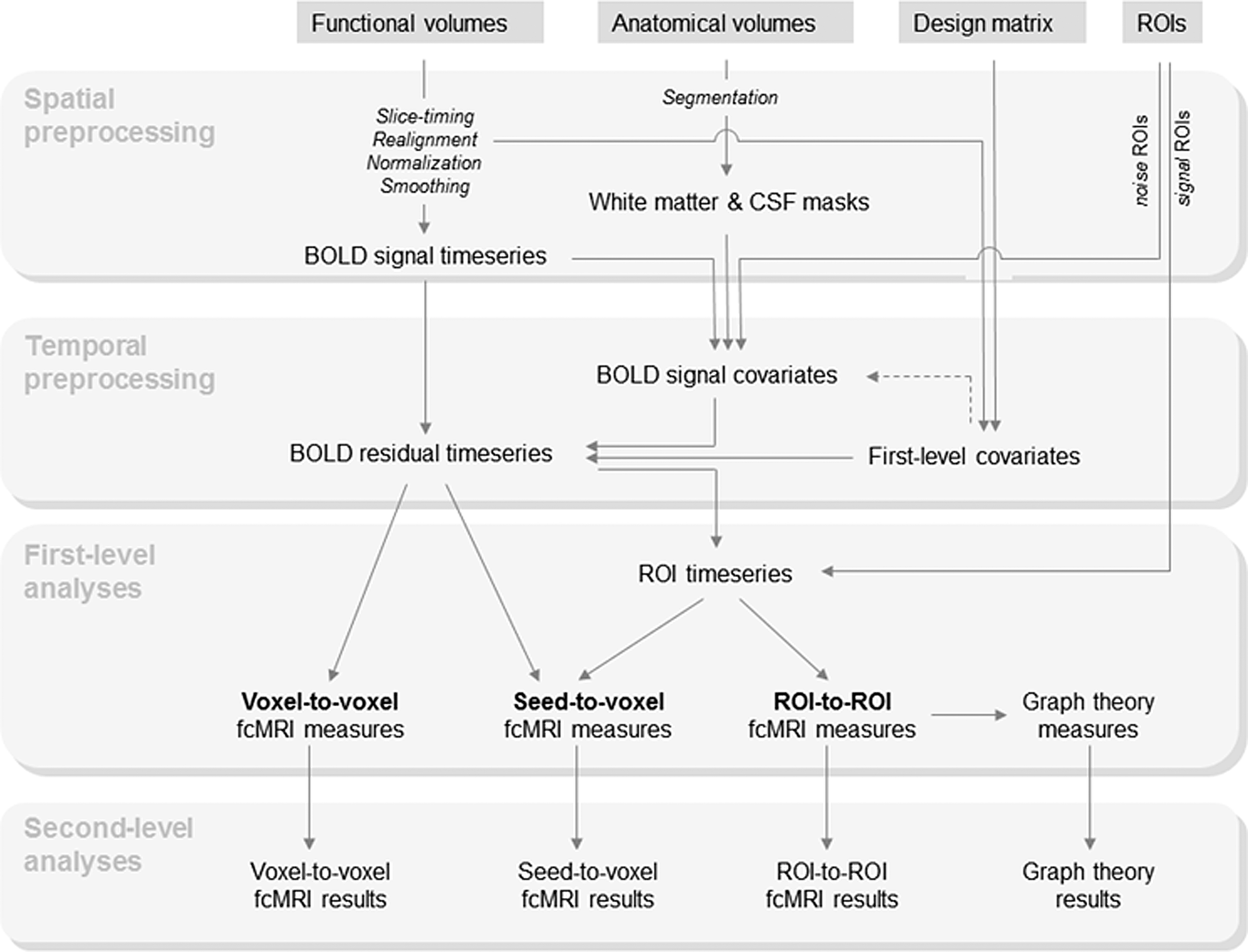
Schematic representation of fcMRI analysis steps. BOLD, blood oxygen level-dependent; CSF, cerebrospinal fluid; fcMRI, functional connectivity magnetic resonance imaging; ROI, region of interest.
Spatial preprocessing
Spatial preprocessing steps for functional connectivity analysis do not typically differ from those used in the context of functional activation analysis. Most fcMRI studies include slice-timing correction, realignment, coregistration and/or normalization, and spatial smoothing. In addition to these steps, the toolbox employs segmentation of gray matter, white matter, and cerebrospinal fluid (CSF) areas for optional use during removal of temporal confounding factors. All spatial preprocessing steps are implemented using SPM8 (Wellcome Department of Imaging Neuroscience, London, UK;
Temporal processing (treatment of temporal confounding factors)
Several studies have emphasized the importance of additional preprocessing steps in fcMRI studies (e.g., Birn et al., 2006; Fox et al., 2005, 2009; Power et al., 2012; Van Dijk et al., 2010; Weissenbacher et al., 2009), including—but not limited to—band-pass filtering and the inclusion of estimated subject motion parameters, artifacts, respiratory and cardiac signals, global BOLD signal, and BOLD signals in white matter and CSF areas as additional covariates. The main concern is that movement and physiological noise sources can potentially induce spurious correlations among distant voxels, increasing the chance of false positives and confounding the interpretation of fcMRI results. These additional preprocessing steps are designed to help mitigate the impact of motion and physiological noise factors, increasing the validity and the robustness of fcMRI analysis.
The toolbox allows the specification of an arbitrary set of possible temporal confounding factors, which can be defined from indirect sources, as subject- and session-specific time series (e.g., estimated subject movement parameters and artifacts, cardiac or respiratory rates, and possible task effects; these are indicated in Figure 1 as Design matrix), as well as BOLD signals obtained from subject-specific noise ROIs (white matter and CSF masks, as well as optionally additional user-defined ROIs). The toolbox implements an anatomical aCompCor strategy (Behzadi et al., 2007) in which a user-defined number of orthogonal time series are estimated using principal component analysis (PCA) of the multivariate BOLD signal within each of these noise ROIs. This strategy generalizes the common practice of extracting the average BOLD time series from one or several seeds located within the white matter and/or CSF areas. In addition, and for each original temporal confounding factor, first- and higher-order derivatives of the associated time series can also be defined by the user as additional confounding factors (e.g., Fox et al., 2005). Each of the defined temporal confounding factors is then regressed from the BOLD time series at each voxel (separately for each session), and the resulting residual time series are band-pass filtered. In particular, the removal of temporal confounding factors, from an observed signal BOLD*(v,t) at voxel v and time t, takes the following form:
where cn (t) represents N temporal confounds defined explicitly through subject- and session-specific time series or implicitly as temporal derivatives of these signals (e.g., subject motion parameters); dkn (t) represents those confounds defined implicitly from K noise ROIs, each characterized by Mk component time series from each noise ROI (e.g., average signal, principal components, or temporal derivatives of these signals within white matter and CSF areas); and an (v) and bkn (v) represent voxel-specific weights for each of these factors estimated using linear regression (see Appendix A.1 for further details of these preprocessing steps).
The toolbox graphical user interface (GUI) encourages users to explore the effect of these additional preprocessing steps by displaying the histogram of voxel-to-voxel functional connectivity values (correlation coefficients between the BOLD time series of a random subset of voxels) before and after regression of the selected temporal confounding factors. This display typically shows a heavily skewed distribution of connectivity values in the presence of motion and/or physiological noise sources, which is approximately centered and normalized by the regression process (Fig. 2). This exploration can help users optimize the choice of preprocessing steps as well as help detect anomalous subjects/sessions.
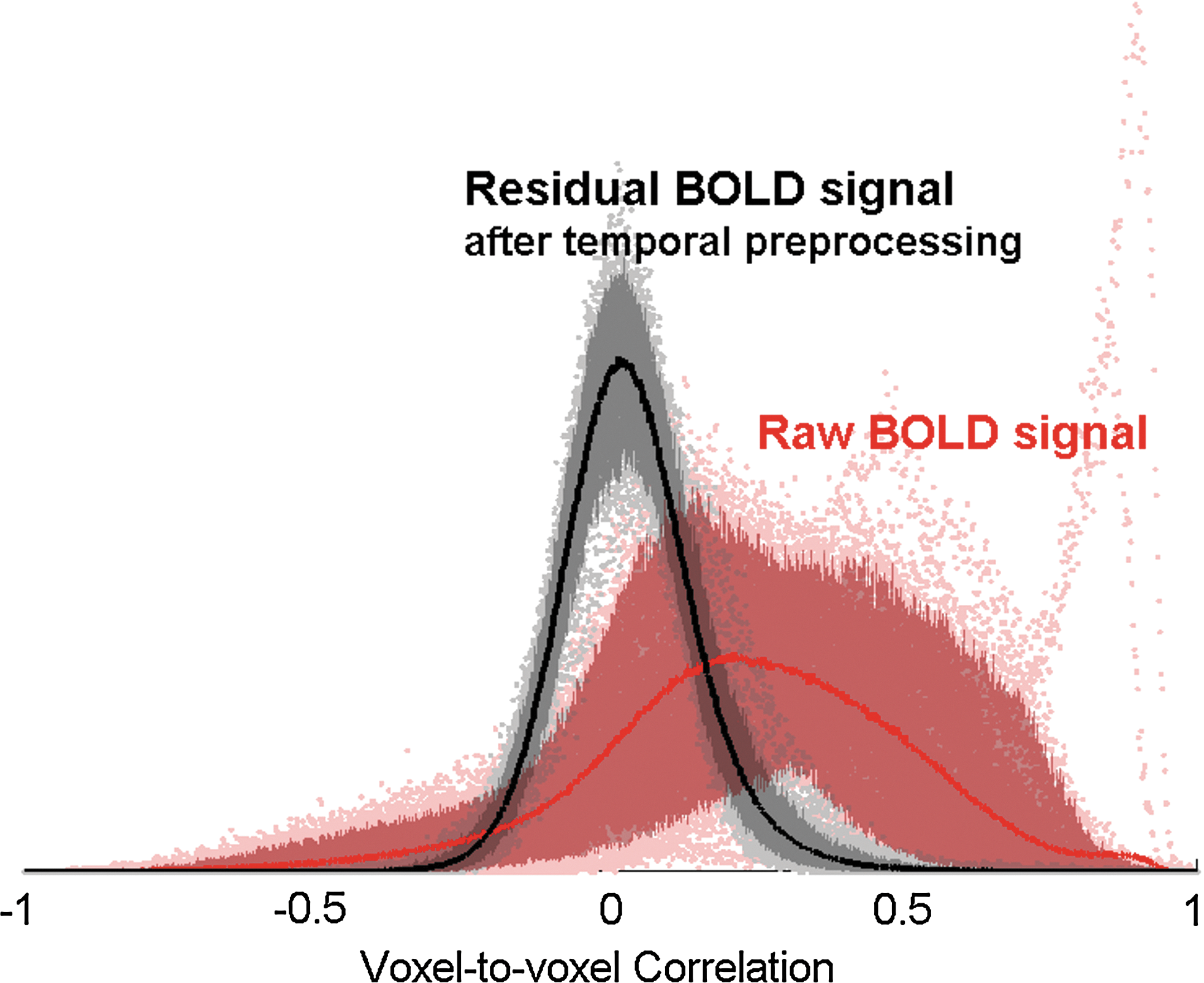
Effect of temporal preprocessing steps on the distribution of voxel-to-voxel BOLD signal correlation values. The average distribution (across subjects and sessions) is shown as thick lines, and its 5% and 95% percentiles are shown as filled areas. After temporal preprocessing, voxel-to-voxel functional connectivity estimates show a reduction in bias and an associated increase in reliability across subjects and sessions (see text for details).
ROI time series
Functional connectivity measures are typically computed either between every pair of voxels (voxel-to-voxel analysis), between a seed voxel or area and every other voxel (seed-to-voxel analysis), or between each pair of seed areas (ROI-to-ROI analysis). The toolbox allows the definition of seed areas using standard practices, including individual mask image volumes [where an ROI is defined by all voxels with values above zero, e.g., WFU pickatlas files (Maldjian et al., 2003) or functional mask files defined using SPM save functionality], text files (listing Montreal Neurological Institute (MNI) coordinates of ROI voxels), and atlas image volumes where multiple ROIs can be jointly defined using a single image volume. Each ROI is characterized by voxels sharing the same identifier number, for example, talairach atlas (Lancaster et al., 2000). ROIs can be defined separately for each subject (subject-specific ROIs) or jointly across all subjects (e.g., MNI space).
The average BOLD time series is computed across all the voxels within each ROI. In addition, the toolbox allows the extraction of additional temporal components from each area resulting from a principal component decomposition of the temporal covariance matrix (as for the noise ROIs above), as well as the estimation of higher-order temporal derivatives of these original BOLD signals. In general the following ROI time series can be computed from each seed area:
BOLD(ν, t): BOLD timeseries at voxel ν and time t
Ω x : voxels in seed area
m: order of PCA component (0 for straight average)
n: order of temporal derivative (0 for original signal)
In combination with the average BOLD signal within an ROI, PCA component signals allow multivariate analysis of functional connectivity patterns. In addition, temporal derivative BOLD signals when used in combination with multivariate measures of connectivity (e.g., multivariate regression or semipartial correlation measures) allow the exploration of temporal lags or more complex linear dynamics between two areas.
Linear fcMRI measures
The toolbox focuses on linear measures of functional connectivity between two sources: zero-lagged bivariate-correlation and bivariate-regression coefficients, and their associated multivariate measures, semipartial-correlation and multivariate-regression coefficients (Table 1). Bivariate correlation and regression coefficients measure the level of linear association of the BOLD time series between each pair of sources when considered in isolation. In contrast, semipartial correlation and multivariate regression coefficients consider multiple sources simultaneously and estimate the unique contribution of each source using a general linear model. In bivariate and semipartial correlation analyses, effect sizes represent correlation coefficients (their values squared can be interpreted as the percentage of the target BOLD signal variance explained by each source BOLD signal). In bivariate and multivariate regression analyses, effect sizes represent % changes in BOLD activity at each target associated with a 1% change of BOLD activity at each source ROI. Before being entered into second-level between-subjects analysis, a Fisher transformation (inverse hyperbolic tangent function) is applied to all bivariate and semipartial correlation measures in order to improve the normality assumptions of standard second-level general linear models.
x and y represent two BOLD time series vectors (centered), X and Y represent matrices created by concatenating horizontally one or several x and y vectors, and the brackets [] represent the operation of zeroing all the nondiagonal elements in a matrix.
Voxel-to-voxel measures
The toolbox also computes a complete voxel-to-voxel functional correlation matrix for each subject. From the residual BOLD time series at every voxel within an a priori gray matter mask (isotropic 2-mm voxels), the matrix of voxel-to-voxel bivariate correlation coefficients is computed. To minimize storage and computation requirements (explicit storage of this matrix could occupy above 300 Gb for each subject), this matrix is instead characterized without loss of precision by its eigenvectors and associated eigenvalues (see Appendix A.2). In addition to downsampling the voxel-to-voxel correlation matrices to any desired target resolution, the toolbox also computes several voxel-level measures of functional connectivity directly from the original voxel-to-voxel correlation matrix (see Table 2). Integrated local correlation (ILC) (Deshpande et al. 2007) characterizes the average local connectivity between each voxel and its neighbors. Radial correlation contrast (RCC) (Goelman, 2004) characterizes the spatial asymmetry of the local connectivity pattern between each voxel and its neighbors. Intrinsic connectivity contrast (ICC) (Martuzzi et al. 2011) and radial similarity contrast (RSC) (Kim et al., 2010) are novel measures similar to ILC and RCC measures, but characterizing the global connectivity pattern between each voxel and the rest of the brain (instead of the local connectivity pattern around each voxel). In particular, ICC characterizes the strength of the global connectivity pattern between each voxel and the rest of the brain, while RSC characterizes the global similarity between the connectivity patterns of neighboring voxels. In addition to these measures the toolbox allows simple and fast implementation of other user-defined voxel-level fcMRI measures, as long as these measures can also be characterized as a function of the eigenvectors/eigenvalues of the voxel-to-voxel correlation matrix. The Illustration of Functional Connectivity Analysis in Conn section [Illustration of voxel-to-voxel analysis (optimal placement of fcMRI seeds) subsection] illustrates the application of one such user-defined measure to investigate between-session similarity of functional connectivity patterns, and Appendix A.2 describes the characterization of this measure as a function of the eigenvectors/eigenvalues of the voxel-to-voxel connectivity matrix.
Integrated local correlation and radial correlation contrast characterize properties of the local pattern of connectivity (between each voxel and its neighbors). Global correlation strength and radial similarity contrast characterize properties of the global pattern of connectivity (between each voxel and the entire brain).
x and y represent the spatial locations of two arbitrary voxels, hσ represents a Gaussian convolution kernel of width σ, and Ω represents the set of all brain voxels.
Task-related and resting state fcMRI
The previous sections characterize the steps necessary to perform first-level (within-subjects) connectivity analysis of resting state BOLD time series, as well as time series derived from the residuals of BOLD time series in block- and event-related designs after removing modeled task or condition effects (Fair et al., 2007) (e.g., simply by including these modeled condition effects as additional temporal confounding factors). The toolbox also allows condition-dependent functional connectivity analysis of block design studies, such as fcMRI analysis of interleaved resting periods or analysis of functional connectivity within task blocks. In these cases and after the session-specific treatment of temporal confounds, the BOLD time series is divided into scans associated with each blocked presentation. To take into account the hemodynamic delay, block regressors for each condition are convolved with a canonical hemodynamic response function, a combination of two gamma functions, and rectified {filtered to keep the positive part of the original time series; y[n]=max(0,x[n])}. All of the scans with nonzero effects in the resulting time series are concatenated for each condition and across all sessions, weighting each scan by the value of these time series. Alternatively it is also possible to use a Hann function (e.g., a “Hann function” window, shaped as a half cycle of a sine-squared function) instead of the rectified hrf function that more heavily de-weights the scans at the beginning and end of each block, as well as to omit any form of within-block weighting. In the case of block design studies, it is also recommended to include standard task regressors (block regressors convolved with a canonical hemodynamic response function) and their first-derivative terms as additional covariates in the temporal preprocessing step. This step helps avoid possible between-condition main effects from affecting within-condition connectivity estimates in the presence of possible voxel-specific differences in hemodynamic delay. Resting state analysis is treated like a special case of task-specific analysis where only one condition spanning the entire scanner acquisition length is considered.
Second-level analysis
Following the computation for each subject of seed-to-voxel connectivity maps, ROI-to-ROI connectivity matrices, and voxel-level fcMRI measures from voxel-to-voxel analysis, each one of these measures can then be entered into a second-level general linear model to obtain population-level estimates and inferences. Specific hypotheses can then be tested using between-subjects contrasts (e.g., comparing functional connectivity patterns between two groups of subjects), between-condition contrasts (e.g., comparing task- or condition-specific connectivity patterns between two conditions), between-source contrasts (e.g., comparing functional connectivity patterns between two seeds), and combinations of these contrasts (e.g., testing group by condition interactions). False positive control in ROI-to-ROI analysis is implemented using uncorrected or false discovery rate (FDR)-corrected p-values. Uncorrected p-values are appropriate when the researcher's original hypotheses involve only the connectivity between two a priori ROIs and FDR-corrected p-values are appropriate when the researcher's original hypotheses involve the connectivity between larger sets of ROIs and do not specify a priori which ROIs are expected to show an effect. False positive control in voxel-level analysis is implemented through a combination of a voxel-level height threshold (defined by uncorrected or FDR-corrected voxel-level p-values) and a cluster-level extent threshold (defined by uncorrected, family wise error [FWE]-corrected, or FDR-corrected cluster-level p-values).
Graph theoretical analysis
The toolbox also computes several graph theoretical measures (Achard and Bullmore, 2007; Bullmore and Sporns, 2009; Latora and Marchiori, 2001; Watts and Strogatz, 1998) characterizing structural properties of the estimated ROI-to-ROI functional connectivity networks, and allows users to perform group-level analysis of these measures. Each subject-specific ROI-to-ROI connectivity matrix is thresholded at a fixed level. This threshold can be based on raw connectivity values, normalized z-scores, or percentile scores (resulting in graphs with fixed network-level cost). Supra-threshold connectivity values define an adjacency matrix characterizing a graph with nodes associated with ROIs, and edges associated with the strength of functional connectivity among these ROIs. For each node n in a graph G, cost is defined as the proportion of connected neighbors, global efficiency is defined as the average inverse shortest path distance from node n to all other nodes in the graph, and local efficiency is defined as the average global efficiency across all nodes in the local subgraph of node n (the subgraph consisting only of nodes neighboring node n). In addition, equivalent network-level summary measures can be defined by averaging across all nodes of the network (Table 3). Population-level inferences on these graph theoretical measures are obtained using a second-level general linear model as in the fcMRI analysis above.
dnm (G) represents the shortest path distance between nodes n and m in graph G, and |G| represents the number of nodes in graph G.
ROI, region of interest.
Illustration of Functional Connectivity Analysis in Conn
In this section several examples of fcMRI analysis performed with Conn are illustrated. These examples are chosen to illustrate some of the standard approaches available for RSFC analysis, as well as to demonstrate the reliability of the functional connectivity measures computed by the Conn toolbox. The analyses were based on a publically available resting state dataset (NYU CSC TestRetest dataset,
Preprocessing of BOLD time courses
Spatial preprocessing of functional volumes included realignment, normalization, and smoothing (8-mm FWHM Gaussian filter), using SPM8 default parameter choices. Anatomical volumes were segmented into gray matter, white matter, and CSF areas, and the resulting masks were eroded (one voxel erosion, isotropic 2-mm voxel size) to minimize partial volume effects. The temporal time series characterizing the estimated subject motion (three-rotation and three-translation parameters, plus another six parameters representing their first-order temporal derivatives), as well as the BOLD time series within the subject-specific white matter mask (three PCA parameters) and CSF mask (three PCA parameters), were used as temporal covariates and removed from the BOLD functional data using linear regression, and the resulting residual BOLD time series were band-pass filtered (0.01 Hz<f<0.10 Hz). Figure 2 illustrates the effect of removing temporal covariates on the distribution of voxel-to-voxel BOLD signal correlation values. A random subset of 256 voxels (the same voxels across subjects and sessions) was used to compute the sample distribution of voxel-to-voxel BOLD signal correlation values separately for each subject and session, before and after removal of the defined temporal covariates.
Estimated voxel-to-voxel correlations using the raw BOLD signals typically show distributions with some degree of positive bias, and with large differences between sessions and subjects. In contrast, after temporal preprocessing, the estimated voxel-to-voxel correlations appear more centered and with very similar distributions across sessions and subjects. To quantify this observation, we computed measures of intersession reliability of the voxel-to-voxel connectivity measures from the raw BOLD signal, and compared them with the same measures after temporal preprocessing. The reliability (average intersession correlation) of the resulting group-level voxel-to-voxel connectivity estimates between randomly selected voxels was r=0.52 from the raw BOLD signal, r=0.62 when using subject motion covariates, and r=0.70 when additionally using CompCor method of white matter and CSF noise covariates, and their corresponding intraclass correlation coefficients (one-way random effects, Shehzad et al. 2009) were 0.22, 0.55, and 0.71, respectively. These results highlight that reliability of group-level voxel-to-voxel connectivity measures increases dramatically with the additional methods of noise reduction implemented in the temporal preprocessing steps of the Conn toolbox, potentially due to their effect reducing physiological and other noise-dependent biases on functional connectivity estimates.
Illustration of seed-to-voxel bivariate correlation analysis
A posterior cingulate cortex (PCC) region [a spherical ROI with MNI coordinates (−6,−52,40) and radius 10 mm (Fox et al., 2005)] was used as the seed. The PCC seed shows positive functional connectivity with a network of default areas (shown in red in Fig. 3 top) and negative functional connectivity (shown in blue) with task-related regions. In addition, three separate within-session estimates of the connectivity strength between the PCC seed and each voxel were computed. These session-specific estimates represent the Fisher-transformed correlation coefficients for each voxel averaged across all subjects and converted back to raw correlation coefficient values. Within-session estimates (Fig. 3) show a high degree of reliability (intersession correlation r=0.95, mean absolute error 0.03) when comparing group-level estimates of functional connectivity strength across repeated runs or sessions. Similarly, high interscan reliability (r=0.97) was found when repeating these analyses using bivariate regression measures instead of bivariate correlation measures.
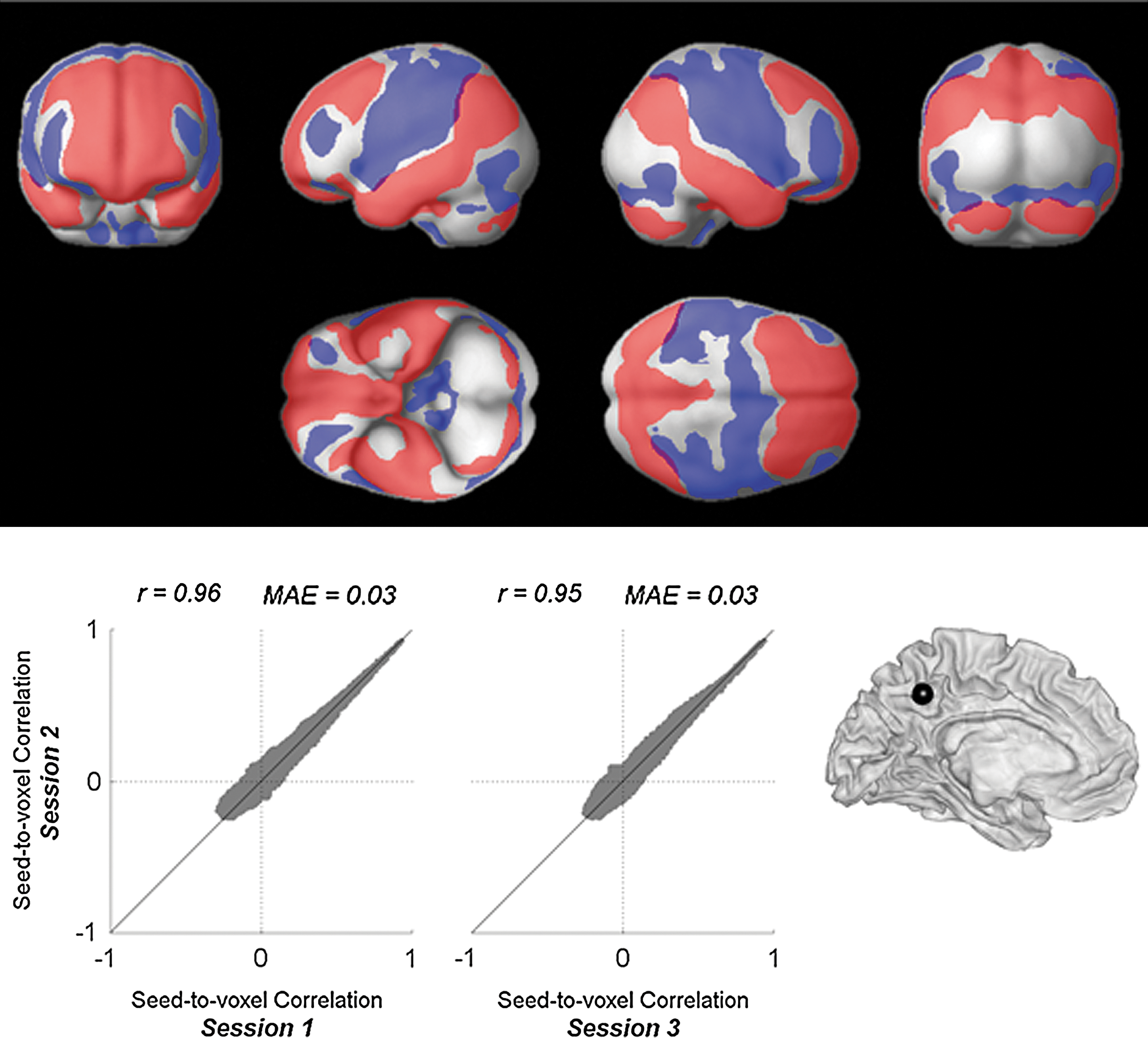
Seed-to-voxel functional connectivity with PCC seed area. Top: Spatial patterns of group-level seed-to-voxel connectivity measures (bivariate correlation) collapsed across the three sessions available from each subject. Red: positive connectivity, blue: negative connectivity. Results are thresholded at FWE-corrected cluster-level p<0.05 (with FDR-corrected two-sided p<0.05 height threshold). Bottom: Intersession reliability. Correlations between session-specific estimates of group-level seed-to-voxel connectivity measures, between session 2 and session 1 (5–11-month difference between the sessions), and between session 2 and session 3 (30-min difference between the sessions). FWE, family wise error; FDR, false discovery rate; PCC, posterior cingulate cortex.
Illustration of seed-to-voxel semipartial correlation analysis
Multivariate seed-to-voxel analysis was also performed to explore the unique connectivity with the PCC area that is not mediated by other default network areas. The average BOLD time series within the PCC area were used as sources of the seed-to-voxel analysis. A multivariate representation of the activation within three control ROIs—medial prefrontal cortex (MPFC), left lateral parietal, and right lateral parietal—characterizing, for each ROI, the average BOLD activation plus four orthogonal components derived from a principal component decomposition of the within-ROI BOLD time series were used as control variables. Semipartial correlation values with the PCC seed were estimated for each voxel. PCC shows unique positive and negative functional connectivity with a large network of areas that are not mediated by other default network regions (Fig. 4). In addition, three separate within-session estimates of the semipartial correlation coefficients between the PCC seed and each voxel were computed. These session-specific estimates represent the Fisher-transformed semipartial correlation coefficients for each voxel averaged across all subjects and converted back to raw correlation coefficient values. Within-session estimates show a high degree of reliability (intersession correlation r=0.82, mean absolute error 0.03) when comparing group-level estimates of unique functional connectivity strength across repeated runs or sessions (Fig. 4). Similar interscan reliability (r=0.88) was found when repeating these analyses using multivariate regression measures instead of semipartial correlation measures.
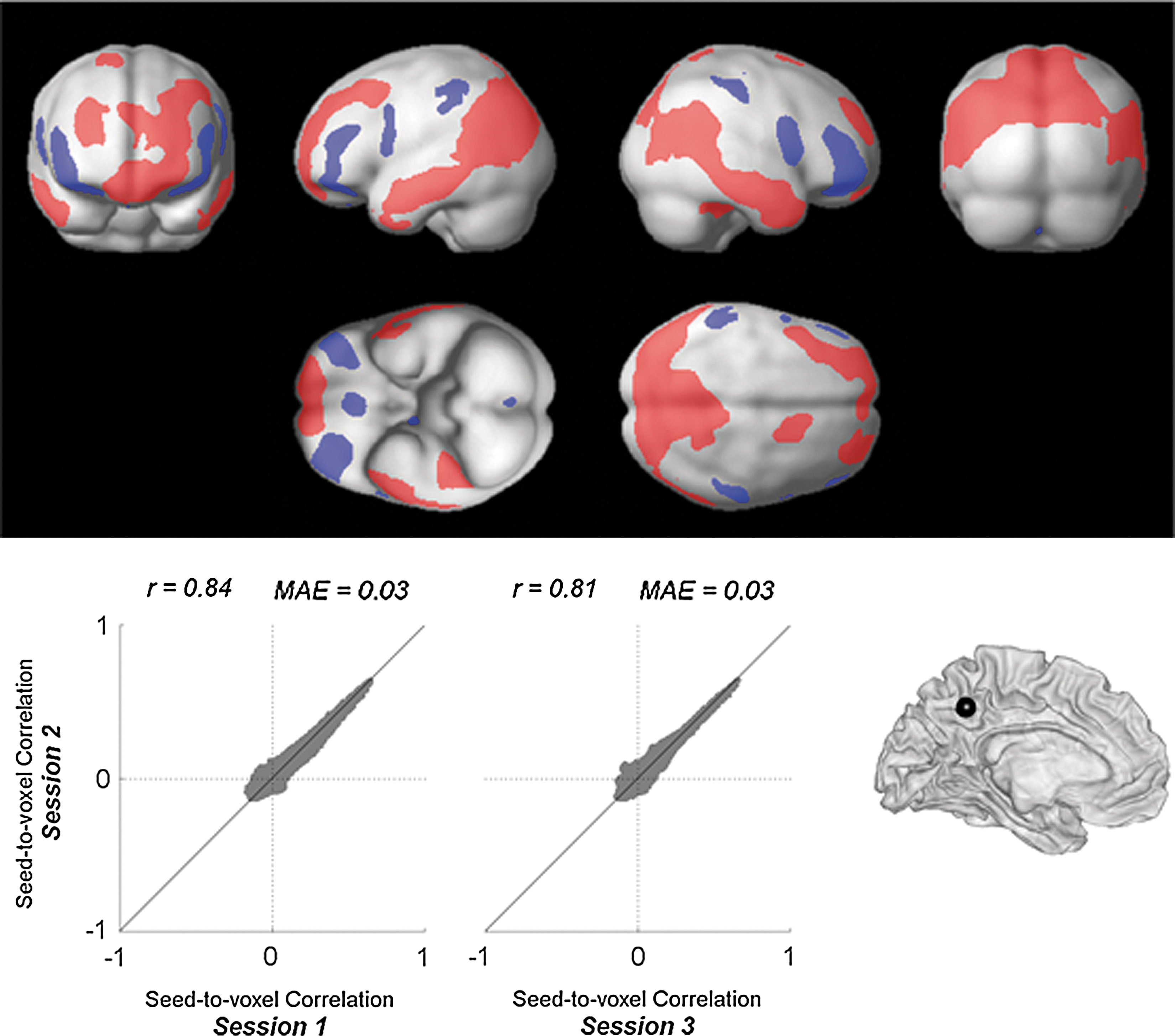
Seed-to-voxel analysis of unique connectivity with PCC seed area (controlled by MPFC, left and right LP). Top: Spatial pattern of group-level effects of the semipartial correlation coefficients collapsed across the three sessions available from each subject. Results are thresholded at FWE-corrected cluster-level p<0.05 (with FDR-corrected two-sided p<0.05 height threshold). Bottom: Intersession reliability of semipartial correlation measures with PCC seed. MPFC, medial prefrontal cortex; LP, lateral parietal.
Illustration of ROI-to-ROI analysis
This analysis uses the same PCC seed area as the previous seed-to-voxel analysis, and estimates the ROI-to-ROI functional connectivity (bivariate correlation measure) between this seed and a set of 84 ROIs defining the Brodmann areas (talairach atlas; Lancaster et al., 2000). Group-level estimates of ROI-to-ROI connectivity show a high degree of reliability (Fig. 5; intersession correlation r=0.99, mean absolute error 0.01). Similar interscan reliability (r=0.98) was found when repeating these analyses using bivariate regression measures instead of bivariate correlation measures.
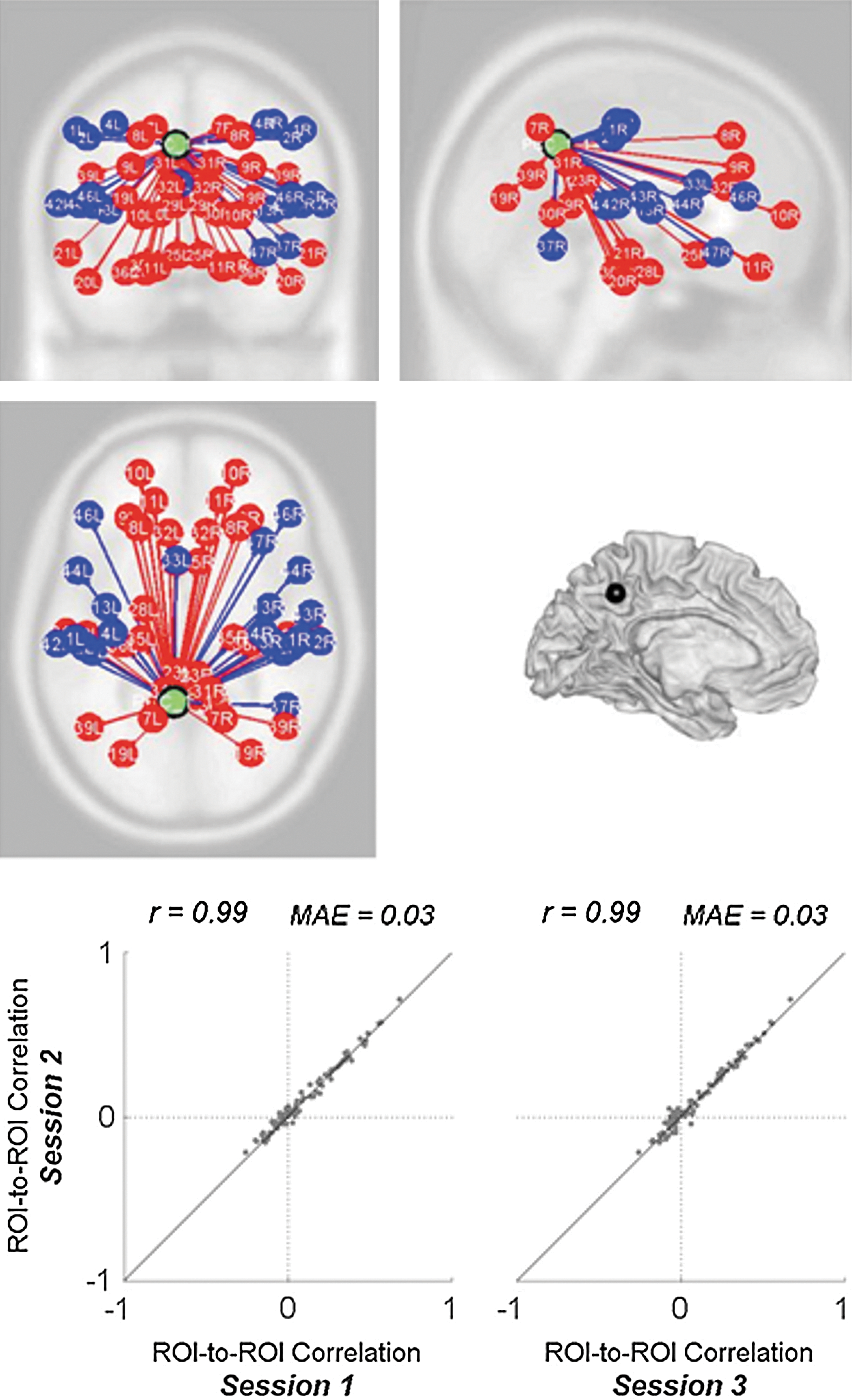
ROI-to-ROI functional connectivity with PCC seed area. Top: ROIs defined from talairach atlas Brodmann areas that show positive (red) and negative (blue) functional connectivity with PCC are shown (for display clarity each ROI is identified by its centroid positions). Results are thresholded at FDR-corrected p<0.05. Bottom: Intersession reliability of ROI-to-ROI group-level functional connectivity measures.
Illustration of graph metrics analysis
The entire matrix of ROI-to-ROI functional connectivity values (bivariate correlation measure) was computed for each subject using the Brodmann area ROIs, and thresholded at a fixed network-level cost value to define an undirected graph characterizing the entire network of functional connections between these ROIs. Negative functional connectivity values were disregarded in these analyses. The network global and local efficiency was computed for a range of possible cost value (K) thresholds and compared to a random graph and to a lattice graph with the same network size and cost (Fig. 6). Small world properties were observed in the range of costs 0.05<K<0.25, where global efficiency is greater than that of a lattice graph and local efficiency is greater than that of a random graph (Achard and Bullmore, 2007). Using an intermediate K=0.15 cost threshold level, the global efficiency of each ROI, a measure of the centrality of each ROI within the network, was computed and averaged across all subjects. This measure showed a high degree of reliability when comparing session-specific estimates of global efficiency across repeated runs or sessions (Fig. 6; intersession correlation r=0.95, mean absolute error 0.01). Similar interscan reliability was found for other graph theoretical measures (local efficiency r=0.90; cost r=0.95).
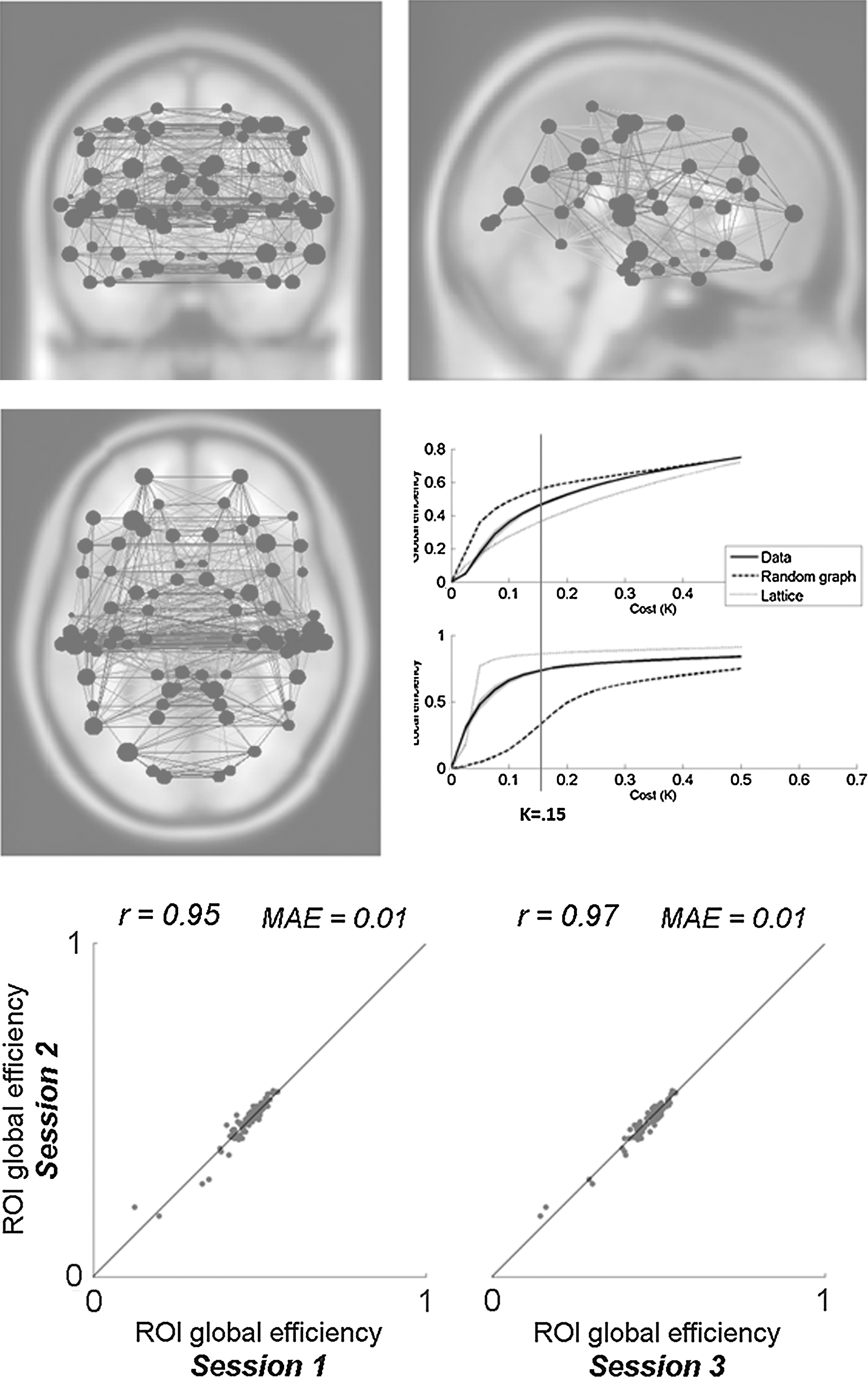
ROI-level analysis of global efficiency. Top: Global efficiency of each ROI (a measure of ROI centrality, and shown proportional to circle sizes in the left display) in the network defined by positively associated ROIs (ROIs defined from talairach atlas Brodmann areas). Small world properties, where global efficiency is greater than that of a lattice graph and local efficiency is greater than that of a random graph, are observed at the chosen cost threshold level (K=0.15). Bottom: Intersession reliability of the estimated group-level measures of global efficiency for each ROI.
Illustration of voxel-to-voxel analysis (RSC)
This analysis investigates the similarity, at each voxel, between the global functional connectivity patterns of this voxel and those of its neighbors. The voxel-to-voxel functional connectivity matrix was computed separately for each session using an isotropic 2-mm voxels within an a priori gray matter mask (SPM apriori/grey.nii mask thresholded at p>0.25; N=212,792 voxels). The RSC measure computes the norm of the difference between the functional connectivity patterns (rows of the voxel-to-voxel matrix) of neighboring voxels. Average group-level RSC across all sessions is shown in Figure 7 (top). Within-session estimates (Fig. 7 bottom) show a high degree of reliability (intersession correlation r=0.98, mean absolute error 0.002) when comparing group-level estimates of RSC across repeated runs or sessions. Similar interscan reliability was found for other voxel-level fcMRI measures derived from voxel-to-voxel analysis (ILC r=0.98; RCC r=0.99; GCS r=0.97).
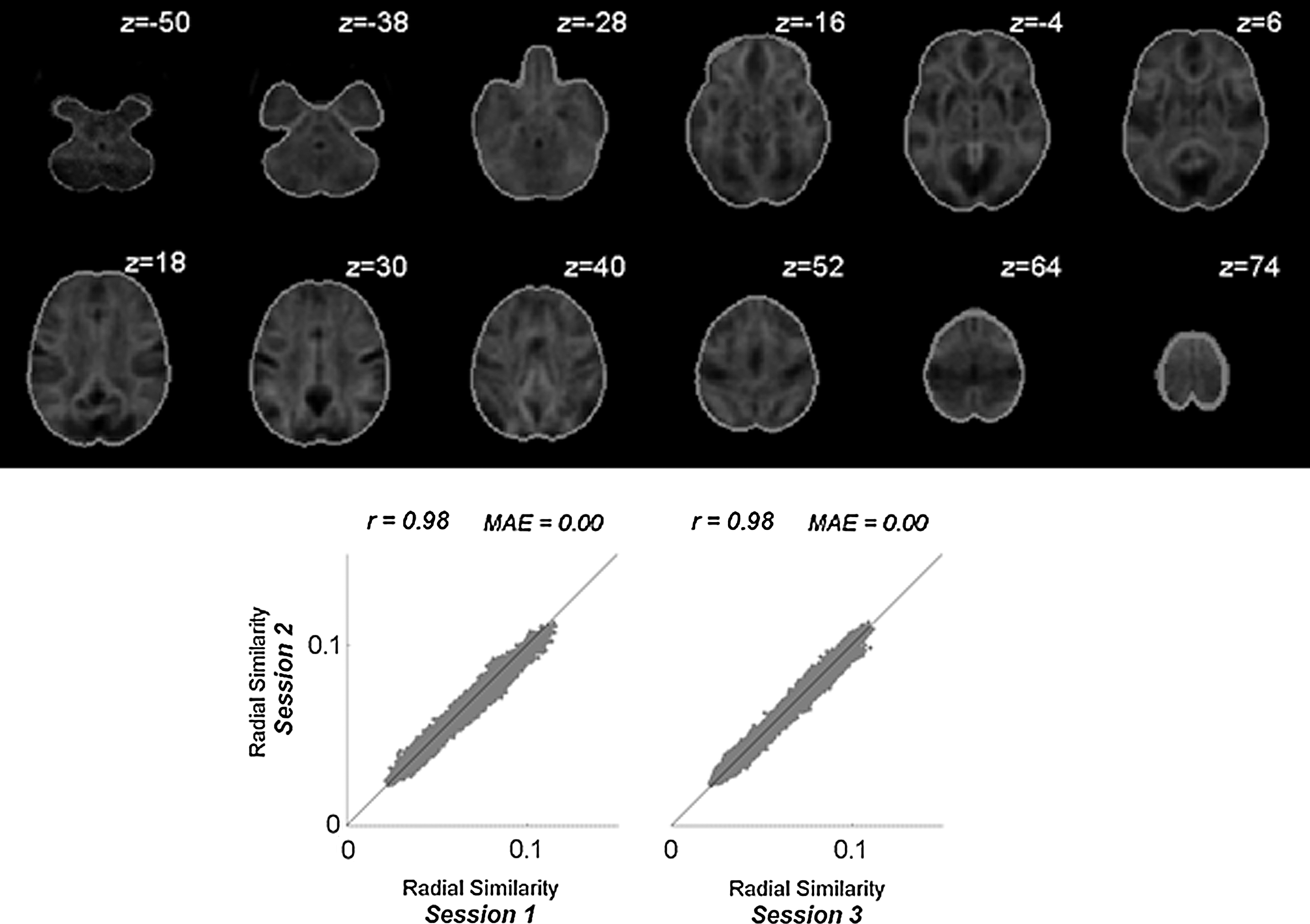
Voxel-to-voxel analysis of radial similarity contrast measure. Top: Average group-level radial similarity contrast at each voxel. Darker shades for a voxel indicate higher similarity between the global functional connectivity patterns of this voxel and those of its neighbors. Bottom: Intersession reliability of the group-level radial similarity contrast measure.
Illustration of voxel-to-voxel analysis (optimal placement of fcMRI seeds)
This analysis investigates the reliability of seed-to-voxel functional connectivity estimates across all possible seed locations. They were implemented as voxel-to-voxel analysis using a user-defined measure characterizing the between-session similarity of functional connectivity patterns at each voxel. Isotropic 2-mm voxels within an a priori gray matter mask (SPM apriori/grey.nii mask thresholded at p>0.25) were used for this analysis (N=212,792 voxels). The matrix of voxel-to-voxel functional connectivity values (bivariate correlation matrix, with size N×N) was parameterized separately for each subject and for each session (Appendix A.2). Separately for each row of this matrix (subject-specific functional connectivity estimates between a given seed voxel and all of the gray matter voxels) the intersession correlation was computed and averaged across each pair of sessions and across all subjects. The resulting measures (for each voxel) characterize the average subject-level intersession reliability of seed-to-voxel analysis when using each voxel as a possible seed location (c.f. group-level reliability measure used in the previous sections) (Fig. 8). Intersession reliability values of subject-level connectivity estimates ranged between r=0.01 and r=0.62 (average r=0.29) across all possible seed locations. Local peaks in this map characterize optimal seed locations (they result in seed-to-voxel functional connectivity patterns that are more robust across sessions than those patterns resulting when using neighboring seed locations). Peak values with intersession reliability above r=0.50 are show in Figure 8 (bottom). Robust seed locations were identified in default network areas—PCC, MPFC, and lateral parietal—in close agreement with standard seed locations for these areas (Fox et al., 2005). In addition, other robust locations included superior temporal gyrus (one anterior temporal source, and a different posterior source close to supramarginal gyrus), superior frontal gyrus, and cingulate gyrus. The results showed high degree of hemispheric symmetry, with all of the peaks (except medial peaks: MPFC, PCC, and cingulate gyrus) having a corresponding peak with similar location and reliability in the opposite hemisphere. Since the seed with highest reliability (0,−56,28) was close but slightly inferior to the a priori PCC seed location used in the previous sections (−6,−52,40), we defined for comparison a new seed location using a spherical ROI of 10 mm centered at the new coordinates (0,−56,28). The group-level and subject-level intersession reliability of the seed-to-voxel functional connectivity estimates when using this new seed definition was r=0.97 and r=0.64, respectively (compared with r=0.95 and r=0.55, respectively, when using the original PCC definition).
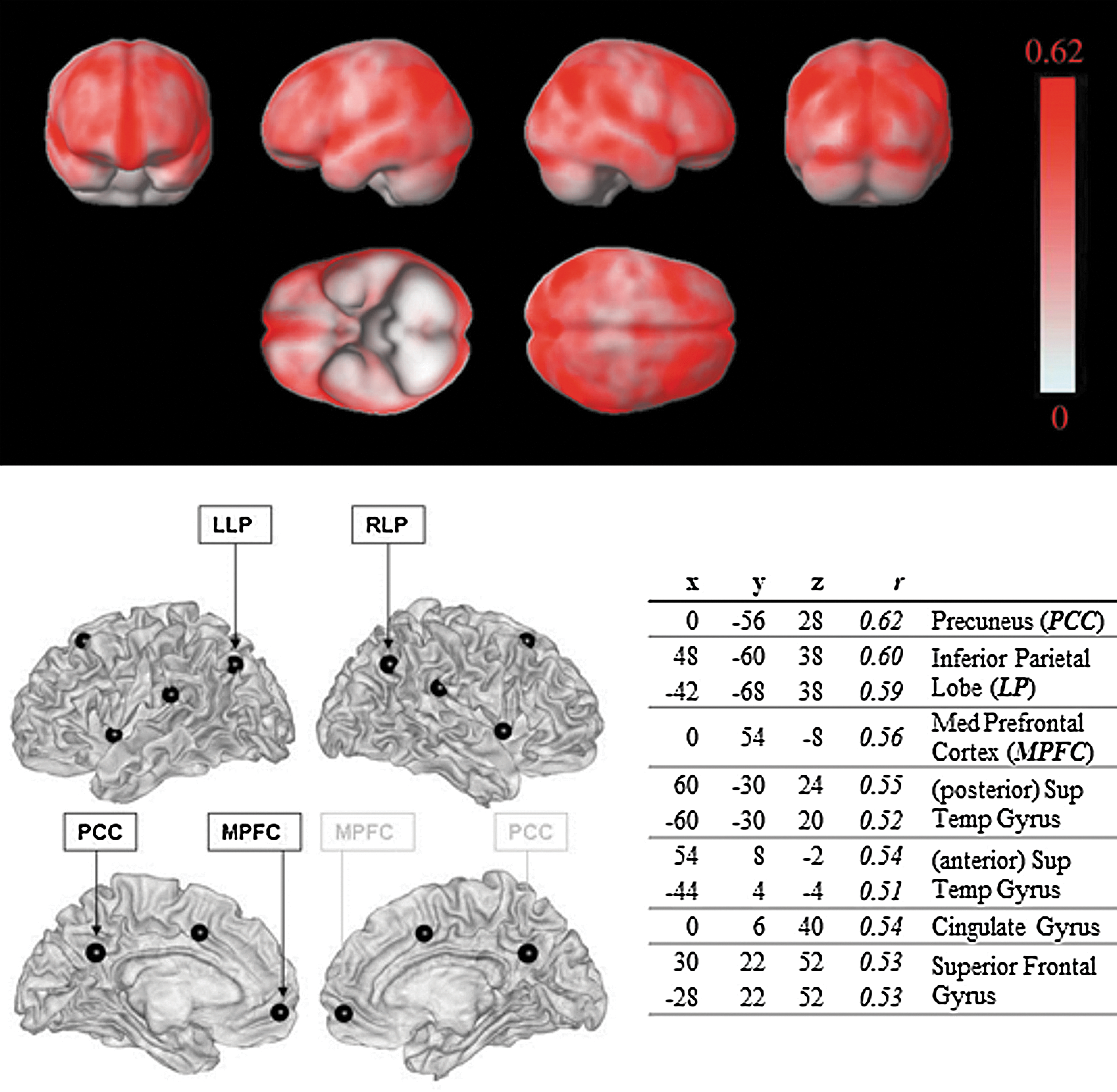
Voxel-to-voxel analysis studying robustness of seed locations. Top: Intersession reliability maps. This display shows the intersession correlation between functional connectivity patterns for all possible seed locations. Darker shades for a voxel indicate that this voxel, when used as seed for standard seed-to-voxel functional connectivity analysis, results in connectivity patterns that are better replicated across sessions (higher intersession correlations). Bottom: Optimal seed locations, as estimated from the local peaks of the reliability maps above. Seed locations that show local maxima in reliability when comparing subject-level estimates of functional connectivity strength across repeated runs or sessions (r value represents the subject-specific intersession correlation averaged across all subjects). All seeds with average r>0.50 are shown. Peak locations are reported as (x,y,z) Montreal Neurological Institute coordinates. LLP, left lateral parietal; RLP, right lateral parietal.
Discussion
RSFC analysis offers an important characterization of functional brain connectivity for both normal and patient populations. This article describes the methods used to compute a variety of functional connectivity measures in the Conn toolbox and illustrates the interscan reliability of these measures. The Conn toolbox offers a large suite of connectivity analyses packaged in a user-friendly GUI. The toolbox can be best used in conjunction with SPM but it is compatible with other analysis packages. The output of most processing and analysis procedures are stored as NIFTI volumes (e.g., the time series post noise reduction and correlation and Z-maps from seed voxel analysis) that may be used for further interrogation. For example, researchers may enter the subject-level Z-maps (Fisher-transformed subject-level correlation coefficients when performing bivariate-correlation analysis) in their analysis package of choice for additional second-level analysis. The toolbox also offers a complete batch processing environment facilitating the implementation of scalable and robust functional connectivity analysis using a simple common framework. In addition, the toolbox encourages users to explore their data at intermediate steps of the analyses (e.g., distribution of voxel-to-voxel connectivity estimates, spatial patterns of potential confounder effects, and individual subject-level connectivity maps), which can aid in detecting and correcting potential anomalies in the data as well as identifying sources of variability that might go unnoticed when focusing on group-level summary results alone.
Anticorrelations
There has been a debate as to whether observed anticorrelations are valid neurophysiological findings or analytic artifacts introduced by global signal regression, a common technique in removing confounds due to physiological and other noise sources in the BOLD time series (Buckner et al., 2008; Fox et al., 2009; Murphy et al., 2009; Weissenbacher et al., 2009). There is general agreement, however, as may be illustrated with mathematical proof, that a seed voxel analysis using global signal regression will necessarily show anticorrelations even if none were truly present in the data because after global regression the distribution of the correlation coefficients between a voxel and every other voxel in the brain is shifted such that the sum ≤0 (Fox et al., 2009; Murphy et al., 2009). Because of this mathematical consequence of the shift in correlation distribution and because the global signal may contain important neural signals as well as noise, it has been recommended to refrain from interpreting anticorrelations when using global signal regression (Chang and Glover, 2009; Murphy et al., 2009).
However, the CompCor method of noise reduction, which does not rely on global signal regression or physiological monitoring, also results in anticorrelations, further supporting a biological basis for their existence, and the positive correlations have higher sensitivity and specificity than global signal regression (Chai et al., 2012). We believe that the CompCorr method, as implemented in Conn, yields valid anticorrelations between large-scale brain networks.
Example illustrations
This article also describes the methods used to compute a variety of functional connectivity measures in the Conn toolbox and illustrates the interscan reliability of these measures. Seed-to-voxel and ROI-to-ROI measures of functional connectivity show high reliability for well-characterized seed locations in RSFC, both when using correlation- and regression-based measures to characterize functional connectivity. Similarly, graph theoretical measures characterizing structural properties of functional connectivity networks, as well as voxel-level measures characterizing the local connectivity patterns (between each voxel and its neighbors) and global connectivity patterns (between each voxel and the rest of the brain) also show high levels of interscan reliability.
Conclusions
The Conn toolbox offers a common framework to define and perform a large suite of connectivity analyses, including bivariate/semipartial correlations, bivariate/multivariate regression, seed-to-voxel connectivity, ROI-ROI connectivity, novel voxel-to-voxel connectivity, and graph theoretical measures for both resting state and task fMRI data. The analyses in this article show high levels of interscan reliability for a variety of fcMRI measures corroborating their potential application as useful neuromarkers. In addition, the Conn implementation of the anatomical CompCor method of noise reduction increases sensitivity and specificity of functional connectivity and allows for better interpretability of anticorrelations as it does not rely on global signal regression. We hope that the imaging community will benefit from the contribution of the tools.
Footnotes
Acknowledgments
The Poitras Center for Affective Disorders Research at the McGovern Institute for Brain Research at MIT supported this work. The authors thank Shay Mozes for initial programming support and John Gabrieli for comments on the article.
Author Disclosure Statement
The authors of the study have no conflict of interest to declare.