Test–Retest Reliability of Graph Theoretic Metrics in Adolescent Brains

Abstract

Graph theory analysis of structural brain networks derived from diffusion tensor imaging (DTI) has become a popular analytical method in neuroscience, enabling advanced investigations of neurological and psychiatric disorders. The purpose of this study was to investigate (1) the effects of edge weighting schemes and (2) the effects of varying interscan periods on graph metrics within the adolescent brain. We compared a binary (B) network definition with three weighting schemes: fractional anisotropy (FA), streamline count, and streamline count with density and length correction (SDL). Two commonly used global and two local graph metrics were examined. The analysis was conducted with two groups of adolescent volunteers who received DTI scans either 12 weeks apart (16.62 ± 1.10 years) or within the same scanning session (30 min apart) (16.65 ± 1.14 years). The intraclass correlation coefficient was used to assess test–retest reliability and the coefficient of variation (CV) was used to assess precision. On average, each edge scheme produced reliable results at both time intervals. Weighted measures outperformed binary measures, with SDL weights producing the most reliable metrics. All edge schemes except FA displayed high CV values, leaving FA as the only edge scheme that consistently showed high precision while also producing reliable results. Overall findings suggest that FA weights are more suited for DTI connectome studies in adolescents.

Introduction

MRI connectomics treats the brain as a network of connections between brain regions. It has been an increasingly popular method for mapping the human connectome, the comprehensive set of structural connections in an individual's brain (Sporns, 2013). Network analysis is carried out using graph theory, which models the brain as a series of nodes and edges (Bullmore and Sporns, 2009; Rubinov and Sporns, 2010). In structural connectivity analysis, network nodes are typically formed from gray matter parcellation into regions-of-interest (ROIs). Edges typically represent white matter tract connections, obtained from diffusion tensor imaging (DTI) and tractography. A connectivity matrix then yields various metrics that can quantitatively describe the brain network's properties and complexity on both a global and local levels. The analysis of such structural networks, and their disruption, has been applied in a variety of neurological disorders, such as Alzheimer's disease (He et al., 2008), amyotrophic lateral sclerosis (Verstraete et al., 2011), temporal lobe epilepsy (Bernhardt et al., 2011), and traumatic brain injury (Caeyenberghs et al., 2012), as well as in psychiatric disorders, such as attention-deficit/hyperactivity disorder (Bos et al., 2017), bipolar disorder (Leow et al., 2013), major depressive disorder (MDD) (Korgaonkar et al., 2014; Tymofiyeva et al., 2017), and schizophrenia (Fornito et al., 2012).

MRI connectomics requires numerous steps with different research groups having their own approaches to this complex analysis (Meskaldji et al., 2013). To rely on a method, it is crucial to examine the reliability of its results. Consequently, there are a growing number of test–retest reliability studies addressing structural brain networks. Previous groups have examined various components of the typical connectomics pipeline, comparing differences in test–retest reliability with respect to global and local graph theory metrics (Andreotti et al., 2014), DTI gradient settings (Vaessen et al., 2010), parcellation schemes (Bassett et al., 2011), tractography algorithms (Bonilha et al., 2015; Buchanan et al., 2014), network sparsity ranges, and the usage of high angular resolution diffusion imaging (Dennis et al., 2012), and more (see the Welton et al., 2015 review). However, few structural connectivity reliability studies have featured comparisons of edge characterization, a critical decision in the overall network construction.

Edges are the connections between network nodes. The simplest criterion for defining an edge is a binary definition: presence or absence. Typically, a fixed threshold or an adaptive threshold (a connectivity matrix density threshold) is set to differentiate between these two states. However, by incorporating additional information, edges can be defined based on their weight (Rubinov and Sporns, 2010). This allows for a more detailed description of the network's properties (Heuvel et al., 2010).

Multiple weighting schemes have been proposed to characterize connectivity in diffusion MRI-based brain networks. Streamline count (SC) is by far the most common edge weighting scheme (Andreotti et al., 2014; Bassett et al., 2011; Buchanan et al., 2014; Hagmann et al., 2007). Variants of this method include normalization by total brain volume and streamline count with density and length correction (SDL) (Buchanan et al., 2014; Cheng et al., 2012; Hagmann et al., 2008). A presumably more biologically meaningful measure of connectivity strength is the measure of fractional anisotropy (FA) sampled along the connecting streamlines. This type of weight is based on tract integrity and myelination, rather than an abstraction of trajectory counts (Rubinov and Bassett, 2011). However, FA-based weighting is less prevalent in test–retest reliability studies. Previous studies have included edge weighting as a comparison to binary definitions, but nearly all employ some variant of SC weighting. Buchanan et al. (2014) were the only group to include FA as an edge weight in their reliability investigation. To address this gap in knowledge, the first aim of our analysis was to compare the test–retest reliability of graph metrics derived from networks constructed using FA- and SC-based weighting schemes. We also included analysis using binary network definitions.

It is also crucial to investigate MRI connectomes' reliability in a demographic where the brain is still developing. Adolescence is a period of ongoing maturation with major global and local white matter network changes (Asato et al., 2010; Barnea-Goraly et al., 2005; Bartzokis et al., 2012; Lebel et al., 2008; Mukherjee et al., 2001; Richmond et al., 2016). There is a concern that longitudinal MRI studies in the still-developing brain might encounter underlying “background” changes (e.g., ongoing myelination or regional differences in gray matter maturation rates, see Khundrakpam et al., 2016), which may influence the findings. In addition, there are many neurodevelopmental and psychiatric disorders the age of onset of which typically occurs in adolescence (Paus et al., 2008). Currently, most reliability studies are based on brain networks created from adult samples. The study by Dennis et al. (2012) was one of the few studies to use a younger cohort, with an average age of 23.6 ± 1.47 years. However, the overall range of this group was large, spanning from 20 to 30 years. Thus, the second aim of our study was to assess the test–retest reliability of graph analysis in the adolescent brain. We examined adolescents at two different interscan periods: (1) 12 weeks apart and (2) 30 min apart, within the same scanning session. In summary, we had two main aims in our test–retest reliability analysis of diffusion MRI connectomics graph metrics. The first aim was to examine differences between binary and weighted edge definitions, and the differences between FA-, SC-, and SDL-weighted edge schemes. The second aim was to investigate the method's reliability in the adolescent brain at two interscan time periods.

Materials and Methods

Subjects

Participants were drawn from a longitudinal study of adolescent volunteers, in which participants received repeated DTI scans. Subjects were grouped based on the time interval between the first and second DTI scans. The first group (n = 26, 16F), of ages ranging from 14.25 to 18.19 years ( \documentclass{aastex}\usepackage{amsbsy}\usepackage{amsfonts}\usepackage{amssymb}\usepackage{bm}\usepackage{mathrsfs}\usepackage{pifont}\usepackage{stmaryrd}\usepackage{textcomp}\usepackage{portland, xspace}\usepackage{amsmath, amsxtra}\usepackage{upgreek}\pagestyle{empty}\DeclareMathSizes{10}{9}{7}{6}\begin{document}$$\bar x$$ \end{document} = 16.62 ± 1.10 years), received scans set 12 weeks apart. The second group (n = 23, 12F), of ages ranging from 14.42 to 18.99 years ( \documentclass{aastex}\usepackage{amsbsy}\usepackage{amsfonts}\usepackage{amssymb}\usepackage{bm}\usepackage{mathrsfs}\usepackage{pifont}\usepackage{stmaryrd}\usepackage{textcomp}\usepackage{portland, xspace}\usepackage{amsmath, amsxtra}\usepackage{upgreek}\pagestyle{empty}\DeclareMathSizes{10}{9}{7}{6}\begin{document}$$\bar x$$ \end{document} = 16.65 ± 1.14 years), received scans within the same session (roughly 30 min apart). All MRI scans were compliant with the Health Insurance Portability and Accountability Act and the study was approved by the Institutional Review Board of the University of California, San Francisco. Written informed consent was obtained from all adult participants or their legal guardians if they were younger than 18 years old. All MRI scans were read by a radiologist (R.D.W.) for incidental findings and participants with abnormal scans were excluded. Participant demographic information is summarized in Table 1, including several participants' psychiatric diagnosis and psychotropic medication status.

Table 1.

Participant Demographics

Interscan period	n	Mean age ± SD (years)	Gender	Diagnosis	Medication
12 Weeks	26	16.62 ± 1.10	16F, 10M	5ADHD	3
30 Minutes	23	16.65 ± 1.14	12F, 11M	5ADHD, 1MDD	4

Participants were volunteers from a longitudinal study of adolescents. Those on medication were taking medication throughout the entire 12-week period.

ADHD, attention-deficit/hyperactivity disorder; F, female; M, male; MDD, major depressive disorder.

MRI data acquisition

Each subject underwent an hour-long MRI protocol using a 3T General Electric MR750 MRI scanner and NOVA Medical 32-channel head coil. The scan included a standard inversion time (T1)-weighted IR-SPGR sequence, with repetition time/TI/echo time (TR/TI/TE) = 10.2 s/450 ms/4.2 s, flip angle = 15°, matrix = 256 × 256, field of view (FOV) = 25.6 cm, and slice thickness = 1 mm. The ASSET acceleration factor was set to 2 with a total scan time of 3 min and 50 sec. The scan also included a spin-echo echo-planar-imaging DTI sequence (TR = 7.5 sec, TE = 60.7 ms, matrix size = 128 × 128, FOV = 25.6 cm, slice thickness = 2 mm). One b ₀ was collected and diffusion-sensitizing gradients were applied at a b-value of 1000 s/mm² along 30 noncollinear directions. The maximum gradient strength was 50 mT/m, and the ASSET acceleration factor was set to 2, resulting in a sequence scan time of 4 min.

MRI data preprocessing

Preprocessing was done using the FMRIB Software Library (FSL 5.0.8) (Smith et al., 2004) and MATLAB. The DTI data were converted to NIFTI (Neuroimaging Informatics Technology Initiative) format. To insure diffusion data quality, an automated data rejection algorithm was used to identify and discard directionally encoded diffusion measurements that were corrupted by motion (Tymofiyeva et al., 2012). When N ≥ 200 pixels deviated from the corresponding mean pixel value for all diffusion directions by three standard deviations, the direction was not included in the tensor calculation. The remaining images were corrected for eddy current distortions and affine head motion using eddy_correct. A b-vector rotation was then applied in MATLAB. The DTI reconstruction and deterministic whole-brain streamline fiber tractography were carried out using Diffusion Toolkit (Wang et al., 2007). The Fiber Assignment by Continuous Tracking (FACT) algorithm (Mori et al., 1999) was used to construct streamlines. This was done with one seed per voxel, using the entire diffusion-weighted volume as a mask image (rather than a thresholded FA map). The Diffusion Toolkit software automatically calculated minimum and maximum thresholds from the mask volume. Streamlines were terminated if the tract curvature exceeded 35°, a value chosen based on previous work in adolescents (Tymofiyeva et al., 2017).

Definition of network nodes

Each brain was segmented into ROIs using the Automated Anatomical Labeling (AAL) atlas (Tzourio-Mazoyer et al., 2002). Only 90 cerebral regions were considered, as the cerebellum is often affected by stronger artifacts and is not always fully covered in the FOV (Tymofiyeva et al., 2017). T1-weighted data were registered to the b ₀-volume of the DTI data set and to the MNI space template using linear registration (FLIRT) (Jenkinson and Smith, 2001; Jenkinson et al., 2002). This allowed for the application of the AAL atlas in the DTI space to produce the 90 nodes of the network. The registration and segmentation results were visually inspected for errors. The resultant ROIs were dilated by one voxel, and they defined the nodes of the graph network analysis.

Definition of network edges

To define the edges (connections) between these nodes (AAL ROIs), three weighting schemes were utilized. Connections were recorded in an n × n adjacency matrix, where a_ij is the edge weight between node i and node j. Only streamlines at least 5 mm in length were considered. The first weighting scheme was defined using the average FA value within voxels along streamlines connecting nodes i and j: \documentclass{aastex}\usepackage{amsbsy}\usepackage{amsfonts}\usepackage{amssymb}\usepackage{bm}\usepackage{mathrsfs}\usepackage{pifont}\usepackage{stmaryrd}\usepackage{textcomp}\usepackage{portland, xspace}\usepackage{amsmath, amsxtra}\usepackage{upgreek}\pagestyle{empty}\DeclareMathSizes{10}{9}{7}{6}\begin{document} \begin{align*}{ a_ { ij } } = { \frac { \mathop \sum \nolimits_ { v \in { V_ { i , j } } } FA \left( v \right) } { { m_ { i , j } } } } , \tag { 1 } \end{align*} \end{document}

where V_i _,j is the set of all voxels (of size m_i _,j) being passed by any of the streamlines that connect nodes i and j. FA is the measure of diffusion anisotropy within the voxel.

The second weighting scheme was defined by SC, the number of tractography streamlines connecting two nodes: \documentclass{aastex}\usepackage{amsbsy}\usepackage{amsfonts}\usepackage{amssymb}\usepackage{bm}\usepackage{mathrsfs}\usepackage{pifont}\usepackage{stmaryrd}\usepackage{textcomp}\usepackage{portland, xspace}\usepackage{amsmath, amsxtra}\usepackage{upgreek}\pagestyle{empty}\DeclareMathSizes{10}{9}{7}{6}\begin{document} \begin{align*}{a_{ij}} = {N_{ij}} , \tag{2} \end{align*} \end{document}

where N_i _,j is the number of all streamlines that connect nodes i and j.

The third edge weight scheme was a variant of SC that corrects for the density and length of a given streamline and is termed streamline density with length (SDL). The SDL scheme is defined as \documentclass{aastex}\usepackage{amsbsy}\usepackage{amsfonts}\usepackage{amssymb}\usepackage{bm}\usepackage{mathrsfs}\usepackage{pifont}\usepackage{stmaryrd}\usepackage{textcomp}\usepackage{portland, xspace}\usepackage{amsmath, amsxtra}\usepackage{upgreek}\pagestyle{empty}\DeclareMathSizes{10}{9}{7}{6}\begin{document} \begin{align*}{ a_ { ij } } = \frac { 2 } { { { g_i } + { g_j } } } \mathop \sum \limits_ { s \in { S_ { ij } } } \frac { 1 } { { l \left( s \right) } } , \tag { 3 } \end{align*} \end{document}

where g_i and g_j are the volumes (number of gray matter voxels) of nodes i and j, S_ij is the set of all streamlines found between nodes i and j, and l(s) is the length of the streamline s connecting nodes i and j. Volume correction helps control for differences in subjects' gray matter volumes, which is proportional to the number of possible connection points per region. Length correction helps to compensate for errors that may increase with tract length and to correct the bias in repeatedly identifying long tracts when conducting white matter seeding (Hagmann et al., 2007).

A fourth binary (B) edge scheme was also studied, representing an unweighted network. The binary scheme used a density threshold value of 15%, applied to SC-weighted matrices. This value was chosen based on a reproducibility analysis by Duda et al. (2014). In their analysis, the mean dice value (signifying consistent network topology) for different fiber tracking algorithms (Euler, FACT, RK4, and TenD) and anatomical label sets (AAL and DTK31) stabilized when using a 15% threshold. The binary entries of the adjacency matrices were calculated by first setting a fixed threshold value for an individual matrix at one streamline and then increasing the fixed threshold value until the density of the remaining nonzero connections constituted 15% of all possible connections in the matrix: \documentclass{aastex}\usepackage{amsbsy}\usepackage{amsfonts}\usepackage{amssymb}\usepackage{bm}\usepackage{mathrsfs}\usepackage{pifont}\usepackage{stmaryrd}\usepackage{textcomp}\usepackage{portland, xspace}\usepackage{amsmath, amsxtra}\usepackage{upgreek}\pagestyle{empty}\DeclareMathSizes{10}{9}{7}{6}\begin{document}$$\left[ {n \left( {n - 1} \right) } \right] / 2$$ \end{document} , where n is the number of nodes (90 in our case).

Results are reported using a combination of the four edge schemes (B, FA, SC, and SDL), and the interscan time interval, 12 weeks (12), or within-session (30). For example, FA30 refers to results based on FA-weighted edges gathered from the within-session scans.

Graph network measures

Four graph network measures were assessed using the Brain Connectivity Toolbox (Rubinov and Sporns, 2010). These metrics were chosen based on their widespread usage in MRI connectomics studies and popularity in test–retest reliability studies (see the Welton et al., 2015 review). The network metrics included two global and two local measures, all constructed multiple times using the four edge characterization schemes (binary, FA-weighted, SC-weighted, and SDL-weighted). Specific descriptions are detailed hereunder. Note that the equations hereunder are for weighted metrics.

Weighted clustering coefficient (c), a measure of a node's connectivity with its neighbors and is one of the most common measures of network segregation. A higher average clustering coefficient value represents increased network segregation. \documentclass{aastex}\usepackage{amsbsy}\usepackage{amsfonts}\usepackage{amssymb}\usepackage{bm}\usepackage{mathrsfs}\usepackage{pifont}\usepackage{stmaryrd}\usepackage{textcomp}\usepackage{portland, xspace}\usepackage{amsmath, amsxtra}\usepackage{upgreek}\pagestyle{empty}\DeclareMathSizes{10}{9}{7}{6}\begin{document} \begin{align*}{ c_i } = \frac { 1 } { { { k_i } \left( { { k_i } - 1 } \right) } } \mathop \sum \limits_ { j , h = 1 } ^n { ( { a_ { ij } } { a_ { ih } } { a_ { jh } } ) ^ { 1 / 3 } } , \tag { 4 } \end{align*} \end{document}

where k_i is the node degree, a basic measure of connectivity defined by \documentclass{aastex}\usepackage{amsbsy}\usepackage{amsfonts}\usepackage{amssymb}\usepackage{bm}\usepackage{mathrsfs}\usepackage{pifont}\usepackage{stmaryrd}\usepackage{textcomp}\usepackage{portland, xspace}\usepackage{amsmath, amsxtra}\usepackage{upgreek}\pagestyle{empty}\DeclareMathSizes{10}{9}{7}{6}\begin{document} \begin{align*}{k_i} = \mathop \sum \limits_{j = 1}^n \left\{ { \begin{matrix} 1 \\ 0 \\ \end{matrix} } \right. \begin{matrix} {{ \rm{ \;if \;}}{a_{ij}}{ \rm{ \;}} > 0} \\ { \;{ \rm{otherwise}}} \\ \end{matrix} . \tag{5} \end{align*} \end{document}

Weighted characteristic path length (l), one of the most widely used measures of network integration. It measures the average shortest path length between all pairs of nodes in the network. \documentclass{aastex}\usepackage{amsbsy}\usepackage{amsfonts}\usepackage{amssymb}\usepackage{bm}\usepackage{mathrsfs}\usepackage{pifont}\usepackage{stmaryrd}\usepackage{textcomp}\usepackage{portland, xspace}\usepackage{amsmath, amsxtra}\usepackage{upgreek}\pagestyle{empty}\DeclareMathSizes{10}{9}{7}{6}\begin{document} \begin{align*}{ l_i } = \frac { 1 } { { \left( { n - 1 } \right) } } \mathop \sum \limits_ { j = 1 , j \ne i } ^n { d_ { ij } } , \tag { 6 } \end{align*} \end{document}

where d is the distance matrix constructed by recording the shortest weighted path length between any pairs of nodes.

Node strength (w), a measure that represents the sum of the edge weights at that node. \documentclass{aastex}\usepackage{amsbsy}\usepackage{amsfonts}\usepackage{amssymb}\usepackage{bm}\usepackage{mathrsfs}\usepackage{pifont}\usepackage{stmaryrd}\usepackage{textcomp}\usepackage{portland, xspace}\usepackage{amsmath, amsxtra}\usepackage{upgreek}\pagestyle{empty}\DeclareMathSizes{10}{9}{7}{6}\begin{document} \begin{align*}{w_i} = \; \mathop \sum \limits_{j = 1}^n {a_{ij}}. \tag{7} \end{align*} \end{document}

A simple connection between two nodes, represented by the connection weight a_ij (defined in Definition of Network Edges section).

The last two metrics are local graph measures. The following regions were examined for node strength: caudate, middle frontal gyrus (MFG), anterior cingulate cortex (ACC), and posterior cingulate cortex (PCC). Regions were selected based on their relevance in neurological and psychiatric disorders (Gasquoine, 2013; Leech and Sharp, 2014; Tymofiyeva et al., 2017). Connections between the caudate to MFG and PCC to MFG were measured for the final graph metric. These were chosen based on their associations with adolescent MDD (Tymofiyeva et al., 2017) and the default mode network (Khalsa et al., 2014), respectively. All local level analyses were conducted bilaterally, with connecting regions on the same side (e.g., L-caudate to L-MFG).

Test–retest statistics

Statistical analyses were carried out in R v.3.4.3 and SPSS v.20. Graph network metrics were assessed with the coefficient of variation (CV) and the intraclass correlation coefficient (ICC) (McGraw and Wong, 1996; Shrout and Fleiss, 1979). The CV is a measure of dispersion relative to the mean and has been implemented in previous test–retest reliability studies (Cheng et al., 2012; Owen et al., 2013; Vaessen et al., 2010). Specifically, we calculated a pooled within-group CV. It is defined as the ratio between the mean within-subject standard deviation \documentclass{aastex}\usepackage{amsbsy}\usepackage{amsfonts}\usepackage{amssymb}\usepackage{bm}\usepackage{mathrsfs}\usepackage{pifont}\usepackage{stmaryrd}\usepackage{textcomp}\usepackage{portland, xspace}\usepackage{amsmath, amsxtra}\usepackage{upgreek}\pagestyle{empty}\DeclareMathSizes{10}{9}{7}{6}\begin{document}$$( {S_w} ) \;$$ \end{document} and the overall measurement mean \documentclass{aastex}\usepackage{amsbsy}\usepackage{amsfonts}\usepackage{amssymb}\usepackage{bm}\usepackage{mathrsfs}\usepackage{pifont}\usepackage{stmaryrd}\usepackage{textcomp}\usepackage{portland, xspace}\usepackage{amsmath, amsxtra}\usepackage{upgreek}\pagestyle{empty}\DeclareMathSizes{10}{9}{7}{6}\begin{document}$$\left( {{ \rm{ \bar y}}} \right)$$ \end{document} , and it is typically expressed as a percentage (Lachin, 2004): \documentclass{aastex}\usepackage{amsbsy}\usepackage{amsfonts}\usepackage{amssymb}\usepackage{bm}\usepackage{mathrsfs}\usepackage{pifont}\usepackage{stmaryrd}\usepackage{textcomp}\usepackage{portland, xspace}\usepackage{amsmath, amsxtra}\usepackage{upgreek}\pagestyle{empty}\DeclareMathSizes{10}{9}{7}{6}\begin{document} \begin{align*} CV = 100* { \frac { { S_w } } { { \rm {y} } } } . \tag { 8 } \end{align*} \end{document}

The ICC was originally created to assess the reliability of multiple raters measuring the same item. It has been previously utilized in other DTI graph theoretic network reliability studies (Andreotti et al., 2014; Bassett et al., 2011; Bonilha et al., 2015; Buchanan et al., 2014; Cheng et al., 2012; Dennis et al., 2012; Owen et al., 2013; Vaessen et al., 2010; for more, see the Welton et al., 2015 review). Specifically, we computed a two-way mixed single measures ICC(3,1), using consistency instead of absolute agreement. “(3,1)” refers to the nomenclature presented by Shrout and Fleiss; the first number refers to the model (3 = two-way mixed-effects) and the second number refers to the type (1 = single rater/measurement) (Koo and Li, 2016). Usage of the term “ICC” in this article can be assumed to mean ICC(3,1). ICCs were calculated from repeated DTI scans for the two groups: (1) 12 weeks apart and (2) 30 min apart (within-session) with the following: \documentclass{aastex}\usepackage{amsbsy}\usepackage{amsfonts}\usepackage{amssymb}\usepackage{bm}\usepackage{mathrsfs}\usepackage{pifont}\usepackage{stmaryrd}\usepackage{textcomp}\usepackage{portland, xspace}\usepackage{amsmath, amsxtra}\usepackage{upgreek}\pagestyle{empty}\DeclareMathSizes{10}{9}{7}{6}\begin{document} \begin{align*}{ \rm { ICC } } \left( { 3 , 1 } \right) = \; { \frac { { \rm { BMS } } - { \rm { EMS } } } { { \rm { BMS } } + \left( { k - 1 } \right) { \rm { EMS } } } } , \tag { 9 } \end{align*} \end{document}

where BMS is the between-subject variance, EMS is the mean square error, and k is the number of raters. In our case, raters correspond to the two repeated measurements. ICC test–retest reliability values are commonly interpreted as poor (<0.40), fair (0.40–0.59), good (0.60–0.74), and excellent (0.75–1.00) (Cicchetti, 1994). In general, CV values can be interpreted as an estimate of a metric's precision within subjects, whereas ICCs are additionally related to differences between subjects. We refer to CV as a measure of precision and ICC as a measure of reliability, although ICC also incorporates precision information. These two measures provide complementary information necessary to assess a method in a comprehensive manner. For example, a graph metric that has a high ICC and a high CV can be interpreted as a measure that is sensitive to individual differences but is not precise (Andreotti et al., 2014; Owen et al., 2013).

To assess potential changes from baseline measurement due to ongoing brain maturation in the adolescent participants, we also performed a paired-sample t-test for all metrics and weighting schemes.

Results

MRI scans were well tolerated by all participants. Overall, the number of rejected directions for both groups ranged from 0 to 12 ( \documentclass{aastex}\usepackage{amsbsy}\usepackage{amsfonts}\usepackage{amssymb}\usepackage{bm}\usepackage{mathrsfs}\usepackage{pifont}\usepackage{stmaryrd}\usepackage{textcomp}\usepackage{portland, xspace}\usepackage{amsmath, amsxtra}\usepackage{upgreek}\pagestyle{empty}\DeclareMathSizes{10}{9}{7}{6}\begin{document}$$\bar x$$ \end{document} = 4.6 ± 3.2 directions) and did not differ significantly between the within-session repeated scans and those repeated 12 weeks apart (paired t-test significance for within-session: p = 0.77 and 12-week: p = 0.39).

Graph theory metrics

Graph metrics were calculated for the two groups (12-week or within-session) using the four edge schemes (binary, FA-weighted, SC-weighted, and SDL-weighted). Figure 1 shows an example of a single subject's tractograms and AAL 90-node network maps obtained from two scans within the same MRI session. Table 2 reports significance values of paired t-tests assessing differences between the 12-week repeated measures. Overall, no differences showed statistical significance.

FIG. 1.

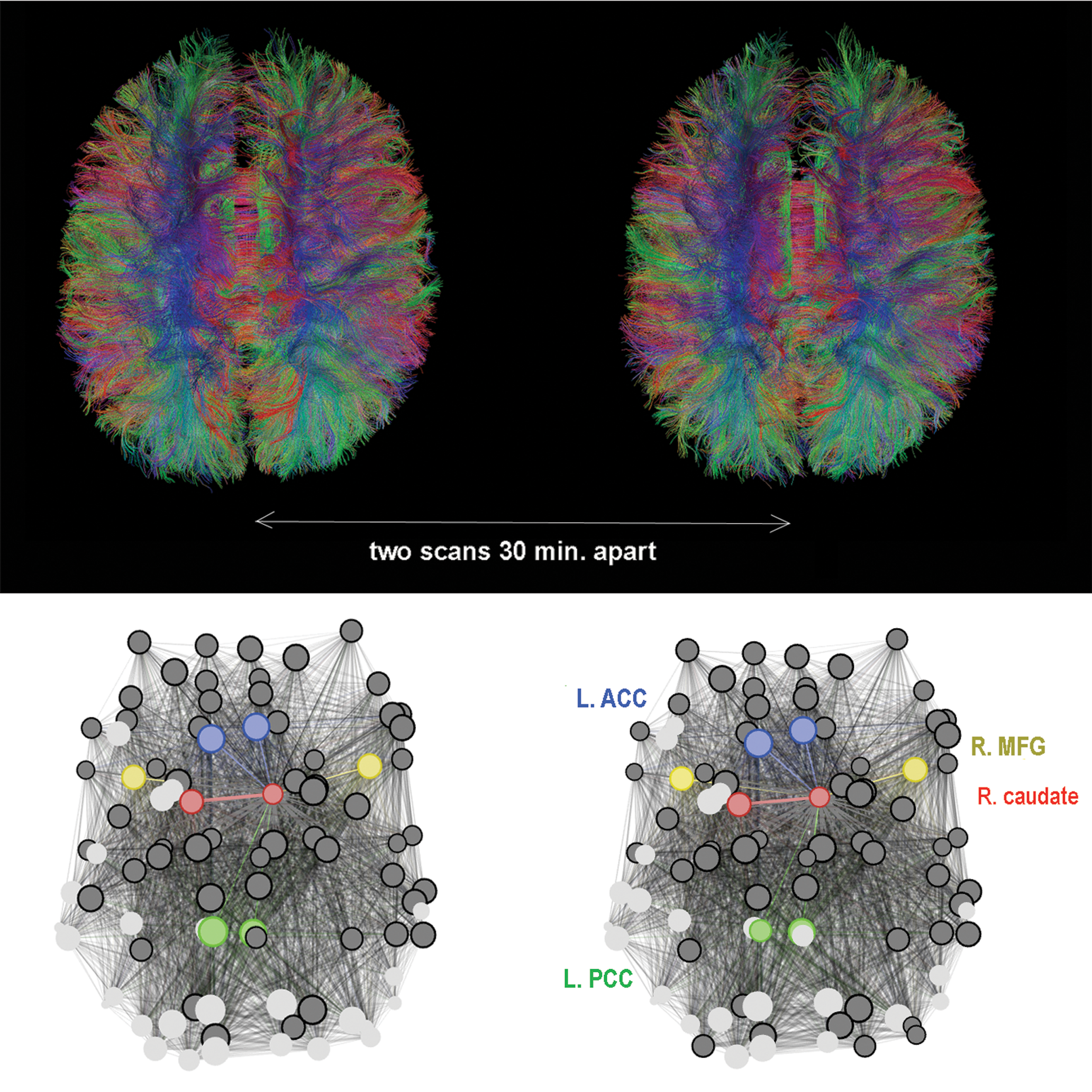
(Top) Tractograms derived from a subject's two DTI scans taken 30 min apart (within-session). (Bottom) A brain network map of the same subject's binary R-caudate node strength. The 90 nodes derived from the AAL atlas are in dark or light gray to reflect presence or absence of an R-caudate connection. The other ROIs of the local graph analysis are also labeled. Network visualization was performed using Gephi (Bastian et al., 2009). AAL, Automated Anatomical Labeling; ACC, anterior cingulate cortex; DTI, diffusion tensor imaging; L., left; MFG, middle frontal gyrus; PCC, posterior cingulate cortex; R, right. Color images are available online.

Table 2.

p-Values Resulting from Paired t-Tests

			Caudate node strength		ACC node strength		MFG node strength		PCC node strength		Caudate to MFG connection		PCC to MFG connection
Edge scheme	Clustering coefficient	Path length	L	R	L	R	L	R	L	R	L	R	L	R
B12	0.14	0.81	0.16	0.33	0.32	0.59	0.55	0.83	0.59	0.13	0.93	0.74	NA	NA
FA12	0.68	0.99	0.30	0.81	0.42	0.66	0.70	0.95	0.22	0.48	0.57	0.19	0.22	0.82
SC12	0.97	0.45	0.40	0.17	0.52	0.28	0.85	0.83	0.76	0.26	0.26	0.24	0.11	0.19
SDL12	0.84	0.80	0.35	0.25	0.41	0.40	0.89	0.95	0.55	0.43	0.35	0.31	0.11	0.19

The 12-week group's graph metrics were tested for differences using a paired t-test (two-tailed). Each row lists an edge scheme's results expressed as a p-value. (B, binary; FA, fractional anisotropy weight; SC, streamline count weight; SDL, streamline count with density and length correction weight), and top-most row denotes graph metrics. ACC, anterior cingulate cortex; L, left; PCC, posterior cingulate cortex; MFG, middle frontal gyrus; R, right. “NA”—PCC to MFG connections were not observed using the binary definition.

Overall, CV values ranged from 1.8% (B30-path length) to 70.4% (SDL12-PCC to MFG,L) and ICC values ranged from 0.10 (SC30-path length) to 0.89 (FA30-Caudate to MFG,L). Both B12 and B30 schemes could not detect direct bilateral PCC to MFG connections, preventing CV and ICC assessments for these specific metrics. In addition, an ICC could not be calculated for the B30 caudate to MFG, R local connection.

On average, graph measures' CV values ranged from 9.6% to 45.0%, and the ICC averages ranged from 0.50 to 0.79 (“fair” to “excellent”). Of the various graph metrics, only the clustering coefficient showed consistent precision (average CV = 9.6%) and consistent reliability (average ICC = 0.66, “good”). The characteristic path length and the local graph metrics showed varying degrees of precision and reliability.

Weighting scheme test–retest statistics

Table 3 gives a summary of the CV analysis for all graph metrics grouped by the four edge schemes and the interscan time intervals. Total weight scheme CV averages (e.g., average of all FA-weighted metrics) were 21.2% ± 16.1%, 7.8% ± 2.6%, 25.2% ± 15.9%, and 27.8% ± 14.2% for B-, FA-, SC-, and SDL-based measures, respectively. As mentioned in Graph Theory Metrics section, B12 and B30 bilateral PCC to MFG connections were not observed; CV could not be calculated for these. A boxplot comparison of the CV values grouped by weighting scheme and time interval is displayed in Figure 2.

FIG. 2.

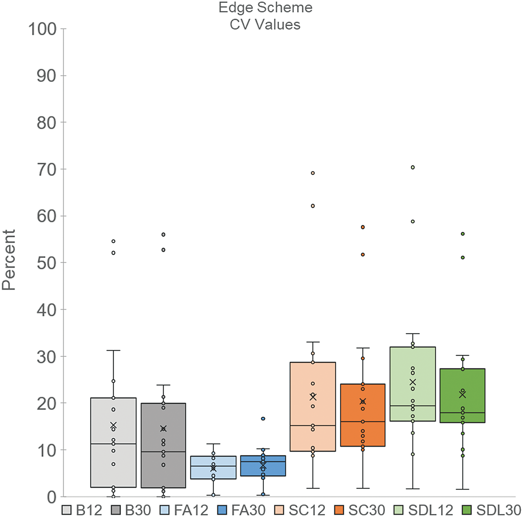
Boxplot comparison of edge schemes' CV values, grouped by time interval. B, binary; CV, coefficient of variation; FA, fractional anisotropy weight; SC, streamline count weight; SDL, streamline count with density and length correction weight; 12, 12-week interval; 30, 30-min within-session interval; x, average CV. Color images are available online.

Table 3.

Coefficient of Variation Values for Weighted and Binary Graph Metrics

			Caudate node strength		ACC node strength		MFG node strength		PCC node strength		Caudate to MFG connection		PCC to MFG connection
Edge scheme	Clustering coefficient	Path length	L	R	L	R	L	R	L	R	L	R	L	R	Mean CV
B12	7.1	1.9	52.1	31.3	18.6	21.1	11.3	11.8	14.4	12.1	54.5	24.7	NA	NA	21.7
B30	6.8	1.8	52.7	23.8	19.0	19.9	12.0	11.2	14.4	9.6	56.0	21.3	NA	NA	20.7
FA12	4.4	3.7	8.6	8.2	7.4	7.3	6.5	6.5	8.7	9.3	6.9	6.0	9.3	11.3	7.4
FA30	5.8	4.0	8.1	8.5	8.6	8.5	8.9	8.7	10.0	10.2	5.1	4.7	7.5	16.7	8.2
SC12	9.7	21.8	30.6	28.7	15.1	19.3	15.5	14.3	10.4	9.9	33.0	24.1	69.2	62.1	26.0
SC30	10.2	20.2	29.5	24.0	18.8	19.1	16.0	14.0	12.9	13.4	31.7	23.0	57.6	51.7	24.5
SDL12	17.2	26.4	31.9	34.8	18.7	23.1	20.5	19.4	16.1	16.2	32.7	27.5	70.4	58.8	29.5
SDL30	15.8	27.3	29.4	27.3	18.8	18.9	16.2	15.9	16.8	17.9	30.2	22.7	56.2	51.1	26.0

CV values are expressed as a percentage.

CV, coefficient of variation; “NA”, PCC to MFG connections were not observed using the binary definition in both interscan time intervals; 12, 12-week interval; 30, 30-min within-session interval.

Table 4 shows a summary of the ICC results. On average, within-session binary-based ICCs (0.66 ± 0.09, “good”) were higher than those from the 12-week interval (0.61 ± 0.14, “good”). FA-weighted ICCs were also higher on average within-session (0.62 ± 0.18, “good”) than those from the 12-week interval (0.54 ± 0.18, “fair”). SC-weighted ICCs were on average lower within-session (0.63 ± 0.17, “good”) than the 12-week interval (0.66 ± 0.13, “good”). SDL-weighted ICCs were also lower on average within-session (0.68 ± 0.10, “good”) than the 12-week interval (0.71 ± 0.11, “good”). Owing to a lack of variance, binary ICC measures could not be calculated for the R-caudate to MFG and bilateral PCC to MFG tracts. Figure 3 shows a boxplot comparison of the ICC values grouped by weighting scheme and time interval.

FIG. 3.

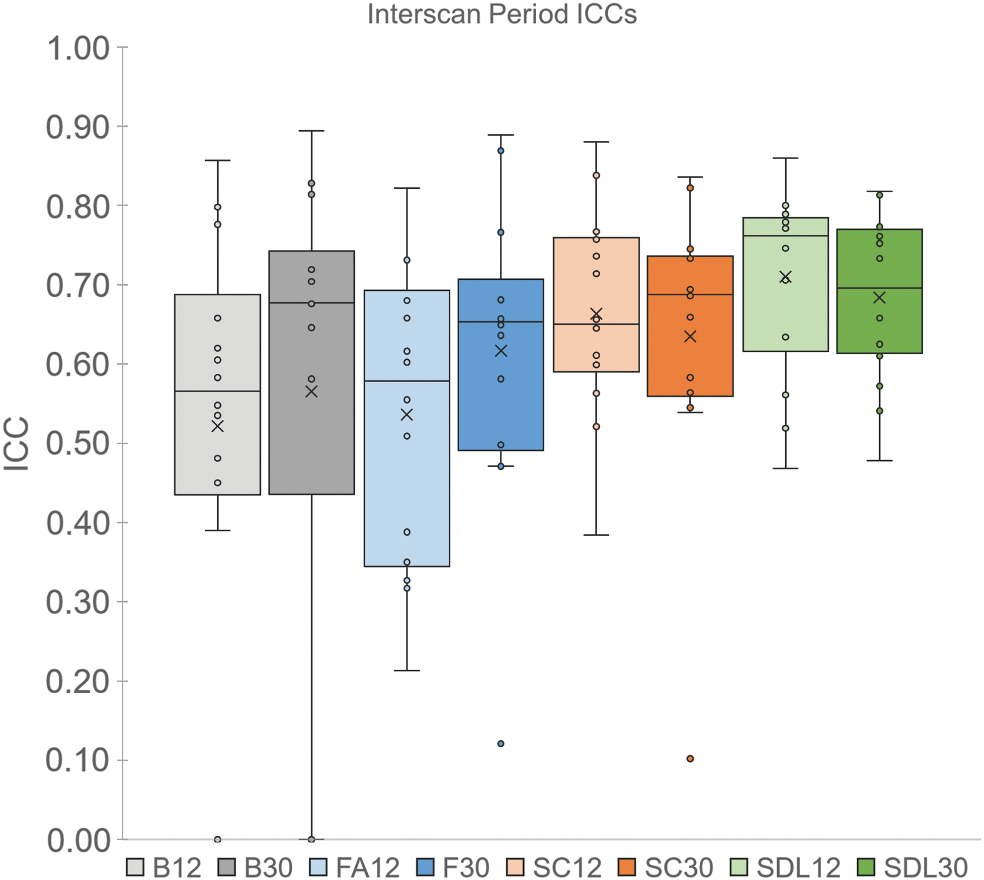
ICC(3,1) results for edge schemes grouped by 12-week and within-session measures. ICC, intraclass correlation coefficient; x, mean ICC value for a particular group of graph theoretical measures. Color images are available online.

Table 4.

ICC(3,1) Values for Weighted and Binary Graph Metrics

			Caudate node strength		ACC node strength		MFG node strength		PCC node strength		Caudate to MFG connection		PCC to MFG connection
Edge scheme	Clustering coefficient	Path length	L	R	L	R	L	R	L	R	L	R	L	R	Mean ICC
B12	0.62	0.55	0.78	0.86	0.39	0.58	0.48	0.45	0.61	0.54	0.80	0.66	NA	NA	0.61
B30	0.68	0.72	0.65	0.68	0.72	0.58	0.83	0.89	0.81	0.70	0.65	NA	NA	NA	0.72
FA12	0.60	0.82	0.33	0.21	0.56	0.68	0.51	0.32	0.74	0.73	0.62	0.39	0.66	0.35	0.54
FA30	0.65	0.87	0.58	0.47	0.64	0.66	0.50	0.47	0.66	0.69	0.89	0.77	0.68	0.12	0.62
SC12	0.66	0.38	0.84	0.77	0.56	0.60	0.61	0.61	0.71	0.76	0.88	0.74	0.52	0.65	0.66
SC30	0.54	0.10	0.69	0.55	0.58	0.56	0.82	0.73	0.69	0.69	0.84	0.66	0.75	0.69	0.63
SDL12	0.77	0.47	0.80	0.78	0.63	0.71	0.75	0.77	0.75	0.79	0.86	0.78	0.52	0.56	0.71
SDL30	0.73	0.48	0.63	0.61	0.57	0.54	0.81	0.77	0.76	0.78	0.82	0.66	0.75	0.66	0.68

ICC analysis could not be conducted for the bilateral binary PCC to MFG connections, and also for B30 R-PCC node strength metric.

ICC, intraclass correlation coefficient.

Interscan period test–retest statistics

Figure 4a–d shows the ICC values (with 95% confidence intervals) of the two interscan periods, separated by edge scheme and the tested graph metrics. The overall average CV percentage for graph measures for the 12-week group was 21.2% ± 16.6%, and the overall average CV percentage for the within-session group was 19.8% ± 14.1%. Average ICC values for the 12-week and within-session repeated measures were 0.63 ± 0.16 (“good”) and 0.66 ± 0.15 (“good”), respectively. Binary and FA-weighted ICCs increased on average as the interscan time interval decreased. SC- and SDL-weighted graph measures did not follow this trend. Refer to Tables 3 and 4 for specific CV and ICC values.

FIG. 4.

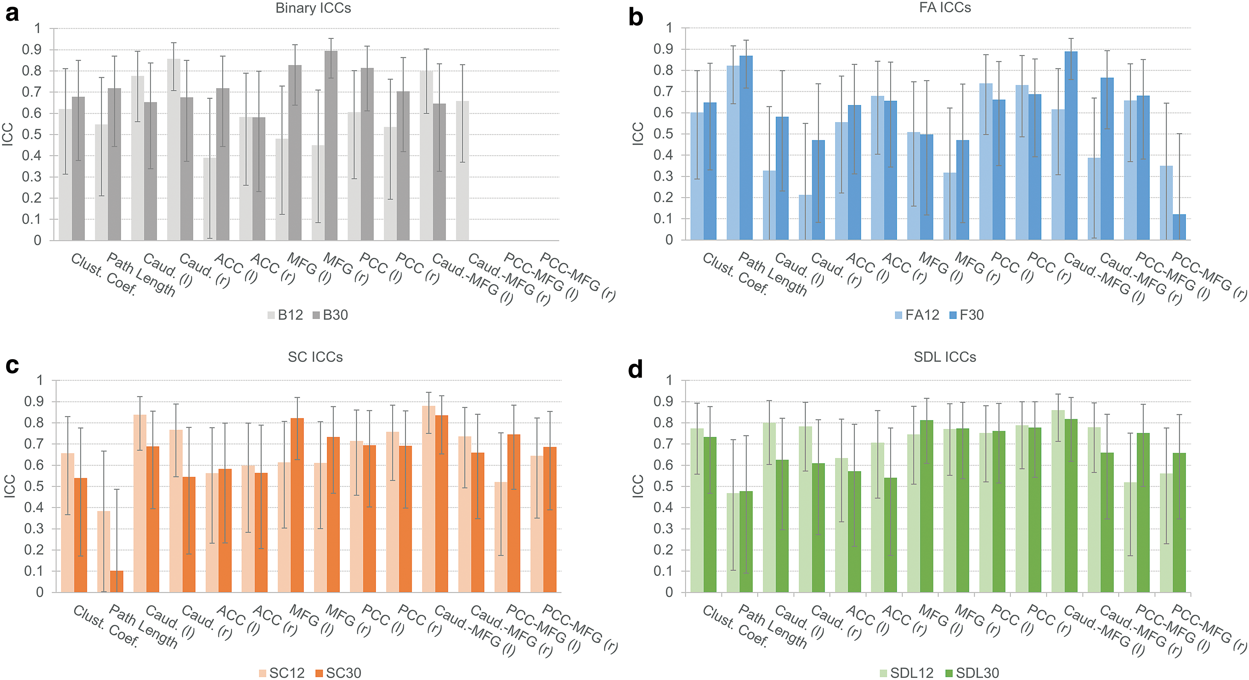
ICC(3,1) results for (a) binary edge definition, (b) FA-weighted definition, (c) SC-weighted definition, and (d) SDL-weighted definition. Each plot displays 12-week (lighter bars) and within-session (darker bars) ICC values for a single edge scheme's network measures. The 95% confidence intervals are also displayed; negative values are treated as a value of 0. Color images are available online.

Healthy subjects test–retest analysis

To exclude potential influence of the illness course and medication on the reproducibility metrics, we also re-examined our 12-week analysis using healthy subjects only. All participants with psychiatric diagnoses were excluded (n = 5), some of whom were on psychotropic medication. The 12-week healthy sample's reliability measures did not differ significantly from the full sample's reliability measures. The average CV values of each edge definition scheme were 22.9% ± 17.3%, 7.2% ± 1.9%, 26.5% ± 18.2%, and 30.2% ± 59.3%, for B, FA, SC, and SDL, respectively. Healthy subjects' average ICC values of each edge definition scheme were 0.61 ± 0.17, 0.59 ± 0.16, 0.66 ± 0.16, and 0.72 ± 0.16, for B, FA, SC, and SDL, respectively. As in the full sample, the ICC for the binary's bilateral PCC–MFG connections lacked variation between groups, preventing an ICC calculation. See Supplementary Tables S1 and S2 for specific results.

Discussion

Our results indicate that overall, graph theory network measures were reliable when derived from structural connectivity in the adolescent brain. Regarding our first aim, network measures derived from nonbinary edge weighting schemes were more consistently reliable and precise than those derived from binary definitions. SC- and SDL-based measures produced the most reliable results, but with consistently low precision. FA-based measures consistently produced very precise graph measures with “fair” to “good” reliability. For our second aim, we found that weighted network measures could produce reliable measurements in the adolescent brain both within session and 12 weeks apart. We discuss next the performance of the studied weighting schemes and differences in reliability and precision of the four studied graph metrics in the following two sections.

Weighting schemes

Our results support previous findings regarding the utility of network weighting in the adult brain (Cheng et al., 2012). We found that binary metrics had decent performance, but the rigidity of the definition (“all or nothing”) led to very inconsistent results with individual weak connections. For example, the B30 R-caudate to MFG measure produced results that suggested subjects' brains were forming or losing connections within the scanning session. Tract formation at this rate is unlikely. It is more likely that the differences between the repeated measures were enough to cross the binary scheme's 15% density threshold. Weighted schemes offer more nuanced characterization of edges that are weak or below the binary threshold (Rubinov and Sporns, 2010). An example of this can be seen in the edge metric between PCC and MFG nodes. The weighted graph metrics characterized these local connections reliably, whereas the binary-based threshold filtered them out.

FA-weighted graph metrics consistently showed high precision in the test–retest analysis. The scheme's average CV was less than half of the others. The FA edge scheme performed better with global measures, particularly characteristic path length. This will be further discussed in Graph Theory Metrics section. FA-weighted metrics were reliable for specific local regions: bilateral ACC, L-MFG, and bilateral PCC, but had trouble with local measures related to the R-caudate and R-MFG.

SC-based graph metrics were all “fair” or higher, able to reliably characterize all local regions and specific connections. The notable exception is its “poor” reliability for path length. Comparatively, the SDL weight did not display this deficiency. Characteristic path length is primarily influenced by long paths between nodes (Rubinov and Sporns, 2010). The tract length correction in the SDL scheme could be causing this higher reliability. The SDL weight had the highest reliability on average, with all graph measures producing reliable results. This finding supports a previous result by Buchanan et al. (2014) in which SDL-weighted global metrics showed slightly better ICCs than FA-weighted ICCs. The authors did find that FA weights were reliable (global ICCs >0.60) as well, which our findings also support.

However reliable, SC- and SDL-weighted measures were hindered by imprecision. Both had CV averages >25%. FA-weighted metrics outperformed all others in this regard. The scheme's high precision and “fair” to “good” average reliability could be due to averaged FA's robustness to noise. Edge weighting by mean diffusion anisotropy could also provide a better reflection of the underlying white matter fiber microstructure (Pierpaoli and Basser, 1996). By comparison, basing the edge weight definition on the number of streamlines is less biologically meaningful. The number of streamlines can change due to tract length, curvature, and degree of branching (Jones et al., 2013).

Graph theory metrics

The clustering coefficient was the graph metric that showed the most consistent reliability and precision. This supports previous findings in other reliable studies (Andreotti et al., 2014; Buchanan et al., 2014; Owen et al., 2013; Vaessen et al., 2010). Seven of the eight clustering coefficient ICCs were “good” or higher (>0.60). CVs for this graph metric were low as well, indicating that the metric could reliably and precisely measure a structural network's segregation with all schemes for 12 weeks.

Characteristic path length has been described as both unreliable and reliable. Studies in the Welton et al., 2015 review reported a large range of ICCs (0.28–0.94; “poor” to “excellent”). Our findings were similarly mixed. Binary and FA-weighted path lengths performed best. Binary edges produced the most precise path length measures (CV <2%), with “fair” (ICC = 0.55) 12-week and “good” (ICC = 0.72) within-session reliability. FA-weighted edges were also very precise (CV ≤4%) and produced “excellent” reliability for both time intervals (ICC = 0.82 and 0.87 for 12-week and within-session repeated measures, respectively). The weight's performance was similar to previous findings by Buchanan et al., although they utilized probabilistic rather than deterministic tractography. Path length did not perform well using the two SC-based weights. Both showed a fourfold increase in CV and reliability scores were “fair” or below.

The local measures in this reliability analysis consisted of node strength and specific connections. The regions were the caudate, ACC, PCC, and MFG, and the individual edges of interest were the caudate to MFG and PCC to MFG. Compared with the global graph analysis, local analysis yielded mixed results. The ICCs ranged from “poor” to “excellent.” Binary-based local measures were particularly variable, with “excellent” ICCs (B12 L-caudate node strength) to an inability to measure tracts (bilateral PCC to MFG). All edge schemes performed reliably with the bilateral PCC node strength and the L-caudate to MFG tract. In this study, all but one edge scheme (B12) had “good” reliability (ICC >0.60). SDL-weighted measures consistently produced “excellent” reliability (ICC ≥0.75), both at 12-week and within-session intervals. However, these reliable local measures were often hindered by low precision (CV >10%). This consistent wide dispersal limits the utility of the SDL edge scheme.

Overall, the global measures outperformed local measures, particularly due to increased precision. This result supports previous findings that local measures displayed more variability than global measures (Andreotti et al., 2014; Cheng et al., 2012). A possible explanation of this finding is that many global network measures are defined as an average of many nodes' local measures. Thus, the global calculation inherently corrects for local variability.

Interscan period analysis

Our second aim was to examine test–retest reliability in the adolescent brain for two interscan periods: within session and 12 weeks apart. This was done by comparing graph metrics with DTI scans 12 weeks apart and within session in adolescents (16.62 ± 1.10 years). Our results indicated that weighted schemes outperformed binary-based definitions. The binary measures failed to identify the PCC-to-MFG connections, whereas the weighted measures were able to. Within the three edge weights, the FA- and SDL-weighted metrics slightly outperformed SC-weighted metrics. However, there was no one scheme that greatly stood out in both precision and reliability. Precision performance remained consistent as before, with FA-weighted metrics outperforming all. There was modest improvement in precision from 12 weeks to within session (CV averages from 21.2% to 19.8%). SC weights and SDL weights showed larger CV improvements, but the metrics remained highly imprecise.

Overall, edge schemes displayed reliable measures both at 12 weeks and within the same scanning session. We expected that reliability would improve when scans were taken closer together. This was the case with binary and FA, but unexpectedly not so with SC and SDL. For example, SC-clustering coefficient decreased from “good” to “fair,” and path length was less reliable within session. FA was the only scheme in which most of the graph coefficients behaved as expected: increasing reliability with decreasing interscan time interval.

There are no comparable reliability results for FA-weighted graph metrics in the literature based on this 12-week interval (in the previously discussed Buchanan et al., 2014 results were for a 2- or 3-day period). However, others have found similarly “good” or higher ICCs for SC-weighted measures over longer durations in adults. For example, Owen et al. (2013) found high reliability for weighted and unweighted metrics for a period of 60.8 ± 33.6 days. In a multisite study, Bonilha et al. (2015) found high ICCs for SC-weighted nodal graph measures for 125 days. Although the methodologies and cohort ages differ, these findings point toward the feasibility of using graph network analysis in studies of longer timescales.

Limitations

There are several limitations in our study that could have affected our results. One such limitation is the varying number of rejected diffusion directions in our data set. Six subjects had 10 or more rejected directions. It has been shown that an increased number of rejected directions can cause an overestimation of FA (Chen et al., 2015). This effect is mainly due to decreased signal-to-noise ratio. Our scanning procedure was representative of typical MRI acquisitions of adolescent populations in both research and clinical settings; motion restriction methods such as a tooth rest were not implemented.

Our analysis is also limited to the chosen graph metrics. Although other graph theoretical measures exist, the chosen four were representative of many graph theory analyses. Another limitation is that the ICCs require a large sample size to generate a precise 95% confidence interval. Reducing the interval's width requires sample sizes challenging to obtain for most MRI studies (Buchanan et al., 2014; Shoukri et al., 2004). We suggest that studies continue using the ICC, implement other metrics in conjunction such as the CV, and aim for larger sample sizes when possible.

Another limitation is related to the fact that many of the referenced test–retest reliability studies employed different methodologies, making proper comparison difficult. One such difference is the usage of a probabilistic tractography approach, rather than a deterministic approach. We chose to use deterministic tractography, since probabilistic tractography has a higher likelihood of generating false positives. This can be more harmful to network analysis than false negatives (Taylor et al., 2017; Zalesky et al., 2016). Importantly, the choice of tractography algorithm has been shown to affect overall reliability results. Buchanan et al. found that probabilistic tractography performed better than deterministic tractography in combination with SDL-weighted measures in terms of mean ICC. However, there were no conclusive advantages when examining FA-weighted measures. Our findings indicate that within a deterministic pipeline setup, FA weighting is a reliable tool for graph network analysis.

Conclusion

This study compared the reliability of graph metrics derived using three weighting schemes (FA, SC, and SDL) and a binary scheme (B). Based on our results, we recommend using weights over binary definitions. We found that FA-based measures produced reliable highly precise graph measures. SC- and SDL-weighted measures produced slightly more reliable results, but they were consistently imprecise. Our findings also indicate that graph analysis is a feasible method over longer periods of time (i.e., 3 months). We also recommend using FA-weighted edge definitions during network construction for this longitudinal context due to its ability to retain its high precision.

Footnotes

Acknowledgments

This study was supported by NCCIH R21AT009173 to O.T., T.T.Y., and E.H.B.; by NICHD R01HD072074 to D.X. and O.T.; by UCSF Research Evaluation and Allocation Committee (REAC) and J. Jacobson Fund to O.T., E.H.B., T.T.Y., and D.X.; by the American Foundation for Suicide Prevention PDF-1-064-13 to T.C.H.; by the Swedish Research Council 350-2012-303 to E.H.B.; and by NIMH R01MH085734 to T.T.Y. The content is solely the responsibility of the authors and does not necessarily represent the official views of the National Institutes of Health or other funding agencies. The funding agencies did not play any role in study design, in the collection, analysis, and interpretation of data, in the writing of the report, and in the decision to submit the article for publication. We would like to thank all the study participants and their parents who made this work possible.

Author Disclosure Statement

No competing financial interests exist.

Supplementary Material

Supplementary Table S1

Supplementary Table S2

References

Andreotti

, Jann

, Melie-Garcia

, Giezendanner

, Dierks

, and Federspiel

. 2014. Repeatability analysis of global and local metrics of brain structural networks. Brain Connect, 4:203–220.

Asato

, Terwilliger

, Woo

, and Luna

. 2010. White matter development in adolescence: a DTI study. Cereb Cortex, 20:2122–2131.

Barnea-Goraly

, Menon

, Eckert

, Tamm

, Bammer

, Karchemskiy

, et al. 2005. White matter development during childhood and adolescence: a cross-sectional diffusion tensor imaging study. Cereb Cortex, 15:1848–1854.

Bartzokis

, Lu

, Heydari

, Couvrette

, Lee

, Kalashyan

, et al. 2012. Multimodal magnetic resonance imaging assessment of white matter aging trajectories over the lifespan of healthy individuals. Biol Psychiatry, 72:1026–1034.

Bassett

, Brown

, Deshpande

, Carlson

, and Grafton

. 2011. Conserved and variable architecture of human white matter connectivity. Neuroimage, 54:1262–1279.

Bastian

, Heymann

, and Jacomy

. 2009. Gephi: an open source software for exploring and manipulating networks. ICWSM, 8:361–362.

Bernhardt

, Chen

, He

, Evans

, and Bernasconi

. 2011. Graph-theoretical analysis reveals disrupted small-world organization of cortical thickness correlation networks in temporal lobe epilepsy. Cereb Cortex, 21:2147–2157.

Bonilha

, Gleichgerrcht

, Fridriksson

, Rorden

, Breedlove

, Nesland

, et al. 2015. Reproducibility of the structural brain connectome derived from diffusion tensor imaging. PLoS One, 10:e01350247.

Bos

, Oranje

, Achterberg

, Vlaskamp

, Ambrosino

, de Reus

, et al. 2017. Structural and functional connectivity in children and adolescents with and without attention deficit/hyperactivity disorder. J Child Psychol Psychiatry, 58:810–818.

10.

Buchanan

, Pernet

, Gorgolewski

, Storkey

, and Bastin

. 2014. Test–retest reliability of structural brain networks from diffusion MRI. Neuroimage, 86:231–243.

11.

Bullmore

, and Sporns

. 2009. Complex brain networks: graph theoretical analysis of structural and functional systems. Nat Rev Neurosci, 10:186–198.

12.

Caeyenberghs

, Leemans

, De Decker

, Heitger

, Drijkoningen

, Linden

, et al. 2012. Brain connectivity and postural control in young traumatic brain injury patients: a diffusion MRI based network analysis. Neuroimage Clin, 1:106–115.

13.

Chen

, Tymofiyeva

, Hess

, and Xu

. 2015. Effects of rejecting diffusion directions on tensor-derived parameters. Neuroimage, 109:160–170.

14.

Cheng

, Wang

, Sheng

, Kronenberger

, Mathews

, Hummer

, and Saykin

. 2012. Characteristics and variability of structural networks derived from diffusion tensor imaging. Neuroimage, 61:1153–1164.

15.

Cicchetti

. 1994. Multiple comparison methods: establishing guidelines for their valid application in neuropsychological research. J Clin Exp Neuropsychol, 16:155–161.

16.

Dennis

, Jahanshad

, Toga

, McMahon

, de Zubicaray

, Martin

, et al. 2012. Test-retest reliability of graph theory measures of structural brain connectivity. Med Image Comput Comput Assist Interv, 15:305.

17.

Duda

, Cook

, and Gee

. 2014. Reproducibility of graph metrics of human brain structural networks. Front Neuroinform, 8:46.

18.

Fornito

, Zalesky

, Pantelis

, and Bullmore

. 2012. Schizophrenia, neuroimaging and connectomics. Neuroimage, 62:2296–2314.

19.

Gasquoine

. 2013. Localization of function in anterior cingulate cortex: from psychosurgery to functional neuroimaging. Neurosci Biobehav Rev, 37:340–348.

20.

Hagmann

, Cammoun

, Gigandet

, Meuli

, Honey

, Wedeen

, and Sporns

. 2008. Mapping the structural core of human cerebral cortex. PLoS Biol, 6:e159.

21.

Hagmann

, Kurant

, Gigandet

, Thiran

, Wedeen

, Meuli

, and Thiran

J.-P

. 2007. Mapping human whole-brain structural networks with diffusion MRI. PLoS One, 2:e597.

22.

, Chen

, and Evans

. 2008. Structural insights into aberrant topological patterns of large-scale cortical networks in Alzheimer's disease. J Neurosci, 28:4756–4766.

23.

Heuvel

, van den, Mandl

RCW

, Stam

, Kahn

, and Pol

HEH

. 2010. Aberrant frontal and temporal complex network structure in Schizophrenia: a graph theoretical analysis. J Neurosci, 30:15915–15926.

24.

Jenkinson

, Bannister

, Brady

, and Smith

. 2002. Improved optimization for the robust and accurate linear registration and motion correction of brain images. Neuroimage, 17:825–841.

25.

Jenkinson

, and Smith

. 2001. A global optimisation method for robust affine registration of brain images. Med Image Anal, 5:143–156.

26.

Jones

, Knösche

, and Turner

. 2013. White matter integrity, fiber count, and other fallacies: the do's and don'ts of diffusion MRI. Neuroimage, 73:239–254.

27.

Khalsa

, Mayhew

, Chechlacz

, Bagary

, and Bagshaw

. 2014. The structural and functional connectivity of the posterior cingulate cortex: comparison between deterministic and probabilistic tractography for the investigation of structure–function relationships. Neuroimage, 102(Part 1):118–127.

28.

Khundrakpam

, Lewis

, Zhao

, Chouinard-Decorte

, and Evans

. 2016. Brain connectivity in normally developing children and adolescents. Neuroimage, 134(Supplement C):192–203.

29.

Koo

, and Li

. 2016. A guideline of selecting and reporting intraclass correlation coefficients for reliability research. J Chiropr Med, 15:155–163.

30.

Korgaonkar

, Fornito

, Williams

, and Grieve

. 2014. Abnormal structural networks characterize major depressive disorder: a connectome analysis. Biol Psychiatry, 76:567–574.

31.

Lachin

. 2004. The role of measurement reliability in clinical trials. Clin Trials, 1:553–566.

32.

Lebel

, Walker

, Leemans

, Phillips

, and Beaulieu

. 2008. Microstructural maturation of the human brain from childhood to adulthood. Neuroimage, 40:1044–1055.

33.

Leech

, and Sharp

. 2014. The role of the posterior cingulate cortex in cognition and disease. Brain, 137:12–32.

34.

Leow

, Ajilore

, Zhan

, Arienzo

, GadElkarim

, Zhang

, et al. 2013. Impaired inter-hemispheric integration in bipolar disorder revealed with brain network analyses. Biol Psychiatry, 73:183–193.

35.

McGraw

, and Wong

. 1996. Forming inferences about some intraclass correlation coefficients. Psychol Methods, 1:30–46.

36.

Meskaldji

, Fischi-Gomez

, Griffa

, Hagmann

, Morgenthaler

, and Thiran

J-P

. 2013. Comparing connectomes across subjects and populations at different scales. Neuroimage, 80:416–425.

37.

Mori

, Crain

, Chacko

, and Van Zijl

PCM

. 1999. Three-dimensional tracking of axonal projections in the brain by magnetic resonance imaging. Ann Neurol, 45:265–269.

38.

Mukherjee

, Miller

, Shimony

, Conturo

, Lee

BCP

, Almli

, and McKinstry

. 2001. Normal brain maturation during childhood: developmental trends characterized with diffusion-tensor MR imaging. Radiology, 221:349–358.

39.

Owen

, Ziv

, Bukshpun

, Pojman

, Wakahiro

, Berman

, et al. 2013. Test-retest reliability of computational network measurements derived from the structural connectome of the human brain. Brain Connect, 3:160–176.

40.

Paus

, Keshavan

, and Giedd

. 2008. Why do many psychiatric disorders emerge during adolescence?. Nat Rev Neurosci, 9:947–957.

41.

Pierpaoli

, and Basser

. 1996. Toward a quantitative assessment of diffusion anisotropy. Magn Reson Med, 36:893–906.

42.

Richmond

, Johnson

, Seal

, Allen

, and Whittle

. 2016. Development of brain networks and relevance of environmental and genetic factors: a systematic review. Neurosci Biobehav Rev, 71:215–239.

43.

Rubinov

, and Bassett

. 2011. Emerging evidence of connectomic abnormalities in Schizophrenia. J Neurosci, 31:6263–6265.

44.

Rubinov

, and Sporns

. 2010. Complex network measures of brain connectivity: uses and interpretations. Neuroimage, 52:1059–1069.

45.

Shoukri

, Asyali

, and Donner

. 2004. Sample size requirements for the design of reliability study: review and new results. Stat Methods Med Res, 13:251–271.

46.

Shrout

, and Fleiss

. 1979. Intraclass correlations: uses in assessing rater reliability. Psychol Bull, 86:420–428.

47.

Smith

, Jenkinson

, Woolrich

, Beckmann

, Behrens

TEJ

, Johansen-Berg

, et al. 2004. Advances in functional and structural MR image analysis and implementation as FSL. Neuroimage, 23 Suppl 1:S208–S219.

48.

Sporns

. 2013. Making sense of brain network data. Nat Methods, 10:491–493.

49.

Taylor

, Wang

, and Kaiser

. 2017. Within brain area tractography suggests local modularity using high resolution connectomics. Sci Rep, 7:srep39859.

50.

Tymofiyeva

, Connolly

, Ho

, Sacchet

, Henje Blom

, LeWinn

, et al. 2017. DTI-based connectome analysis of adolescents with major depressive disorder reveals hypoconnectivity of the right caudate. J Affect Disord, 207:18–25.

51.

Tymofiyeva

, Hess

, Ziv

, Tian

, Bonifacio

, McQuillen

, et al. 2012. Towards the “Baby Connectome”: mapping the structural connectivity of the newborn brain. PLoS One, 7:e31029.

52.

Tzourio-Mazoyer

, Landeau

, Papathanassiou

, Crivello

, Etard

, Delcroix

, et al. 2002. Automated anatomical labeling of activations in SPM using a macroscopic anatomical parcellation of the MNI MRI single-subject brain. Neuroimage, 15:273–289.

53.

Vaessen

, Hofman

PAM

, Tijssen

, Aldenkamp

, Jansen

JFA

, and Backes

. 2010. The effect and reproducibility of different clinical DTI gradient sets on small world brain connectivity measures. Neuroimage, 51:1106–1116.

54.

Verstraete

, Veldink

, Mandl

RCW

, Berg

, van den, and Heuvel

, van den. 2011. Impaired structural motor connectome in amyotrophic lateral sclerosis. PLoS One, 6:e24239.

55.

Wang

, Benner

, Sorensen

, and Wedeen

. 2007. Diffusion toolkit: a software package for diffusion imaging data processing and tractography. Proc Intl Soc Mag Reson Med, 15:3720.

56.

Welton

, Kent

, Auer

, and Dineen

. 2015. Reproducibility of graph-theoretic brain network metrics: a systematic review. Brain Connect, 5:193–202.

57.

Zalesky

, Fornito

, Cocchi

, Gollo

, van den Heuvel

, and Breakspear

. 2016. Connectome sensitivity or specificity: which is more important?. Neuroimage, 142:407–420.

Supplementary Material

Please find the following supplemental material available below.

For Open Access articles published under a Creative Commons License, all supplemental material carries the same license as the article it is associated with.

For non-Open Access articles published, all supplemental material carries a non-exclusive license, and permission requests for re-use of supplemental material or any part of supplemental material shall be sent directly to the copyright owner as specified in the copyright notice associated with the article.

0.00 MB

0.02 MB