Machine Learning Evidence for Sex Differences Consistently Influences Resting-State Functional Magnetic Resonance Imaging Fluctuations Across Multiple Independently Acquired Data Sets

Abstract

Background/Introduction:

Sex classification using functional connectivity from resting-state functional magnetic resonance imaging (rs-fMRI) has shown promising results. This suggested that sex difference might also be embedded in the blood-oxygen-level-dependent properties such as the amplitude of low-frequency fluctuation (ALFF) and the fraction of ALFF (fALFF). This study comprehensively investigates sex differences using a reliable and explainable machine learning (ML) pipeline. Five independent cohorts of rs-fMRI with over than 5500 samples were used to assess sex classification performance and map the spatial distribution of the important brain regions.

Methods:

Five rs-fMRI samples were used to extract ALFF and fALFF features from predefined brain parcellations and then were fed into an unbiased and explainable ML pipeline with a wide range of methods. The pipeline comprehensively assessed unbiased performance for within-sample and across-sample validation. In addition, the parcellation effect, classifier selection, scanning length, spatial distribution, reproducibility, and feature importance were analyzed and evaluated thoroughly in the study.

Results:

The results demonstrated high sex classification accuracies from healthy adults (area under the curve >0.89), while degrading for nonhealthy subjects. Sex classification showed moderate to good intraclass correlation coefficient based on parcellation. Linear classifiers outperform nonlinear classifiers. Sex differences could be detected even with a short rs-fMRI scan (e.g., 2 min). The spatial distribution of important features overlaps with previous results from studies.

Discussion:

Sex differences are consistent in rs-fMRI and should be considered seriously in any study design, analysis, or interpretation. Features that discriminate males and females were found to be distributed across several different brain regions, suggesting a complex mosaic for sex differences in rs-fMRI.

Impact statement

The presented study unraveled that sex differences are embedded in the blood-oxygen-level dependent (BOLD) and can be predicted using unbiased and explainable machine learning pipeline. The study revealed that psychiatric disorders and demographics might influence the BOLD signal and interact with the classification of sex. The spatial distribution of the important features presented here supports the notion that the brain is a mosaic of male and female features. The findings emphasize the importance of controlling for sex when conducting brain imaging analysis. In addition, the presented framework can be adapted to classify other variables from resting-state BOLD signals.

Introduction

Resting-state functional magnetic resonance imaging (rs-fMRI) is a noninvasive approach allowing for studies of brain functions by measuring hemodynamic flow within the resting brain. rs-fMRI has been proven to be an effective approach to discovering and studying consistent brain functional network organization (Biswal, 2012; Damoiseaux et al., 2006; Mantini et al., 2007). In particular, rs-fMRI has been used to identify differences across subjects based on demographic data and biological factors, including gender. Many studies have identified differences between males and females in terms of cognitive performance (Miller and Halpern, 2014), but these results do not provide a comprehensive and consistent view of sex differences (Del Giudice, 2009; Hyde and Plant, 1995).

While there has been evidence of sex differences in some cognitive processes such as language and emotional processing (Besson et al., 2002; Schirmer et al., 2005a,b), other works could not find any conclusive evidence of such differences (Russell et al., 2007; Wallentin, 2009). Similar to functional organization, sex differences were found in the structural organization of the brain (Chekroud et al., 2016; Del Giudice et al., 2016; Rosenblatt, 2016). Research has shown that males have larger total brain volume, gray matter, and white matter tissues (Ingalhalikar et al., 2014). Also, intra- and interhemispheric connections have been shown to vary between males and females, with a tendency for males to have a higher intrahemispheric connectivity (Ingalhalikar et al., 2014). In contrast, females showed high interhemispheric connectivity (Ingalhalikar et al., 2014).

Moreover, brain regions such as the insula, amygdala, and hippocampus have also been shown to structurally differ based on sex (Ruigrok et al., 2014). Similarly, authors in Liu and colleagues (2020) reported consistent sex differences of gray matter volume (GMV) in the cortex and subcortical foci, brain regions associated with social and reproductive behaviors. This study also demonstrated a strong spatial coupling between brain regions showing GMV differences and brain expression of sex chromosome genes in adulthood. Despite the evidence of the brain structural differences, others have argued that both brain and behavior sex differences can be described as a mosaic of male and female properties with no clear binary distinction (Joel and Fausto-Sterling, 2016; Joel et al., 2015). Similarly, fMRI functional connectivity (FC) has been widely used to study sex differences. For instance, Bluhm and colleagues (2008) reported an overall higher FC within the default mode network (DMN) in the medial prefrontal and posterior cingulate cortices in females. Other works showed a stronger internetwork FC in males and a stronger intranetwork FC in females (Allen et al., 2011). While there is a lot of other evidence about sex differences in the resting-state connectivity (Biswal et al., 2010; Tian et al., 2011; Zuo et al., 2010b), other works did not replicate nor consistently find any sex effects (Weis et al., 2019; Weissman-Fogel et al., 2010).

Thus, investigating sex differences at the level of blood-oxygen-level-dependent (BOLD) fluctuation may reveal if there is strong evidence of sex differences. Recently, machine learning (ML) techniques have been used widely to perform classification and regression on neuroscience data (Al Zoubi et al., 2018a,b; Campbell et al., 2020; Cohen et al., 2020; Du et al., 2018; Garner et al., 2019; Kazeminejad and Sotero, 2019; Saccà et al., 2019). Some works focused on using ML for classifying subjects into male and female using functional (Dhamala et al., 2020; Ktena et al., 2018; Smith et al., 2013; Weis et al., 2020; Zhang et al., 2018) and structural data (Chekroud et al., 2016; Feis et al., 2013; Rosenblatt, 2016). In this work, we focused on investigating sex classification using intrinsic BOLD fMRI signal fluctuations. BOLD-derived features have been shown to entertain higher heritability than FC. Thus, we further focus our analysis on BOLD-derived features (Elliott et al., 2018; Smith et al., 2021). More specifically, BOLD can be characterized by the amplitude of the low-frequency fluctuation (ALFF) (Yu-Feng et al., 2007), which measures the extent of spontaneous fluctuation of the BOLD signal.

ALFF has been linked to low-frequency oscillations from spontaneous neuronal activity and may manifest in the rhythmic activity and interaction of processing information across the brain (Cordes et al., 2001). ALFF is calculated by computing the power of the signal within [0.01–0.08] Hz or [0.01–0.1] Hz ranges (Li et al., 2017; Yu-Feng et al., 2007). In addition, other information can be derived from BOLD fluctuation such as the fraction of ALFF (fALFF), which is defined as the ratio of the power within [0.01–0.08] Hz or [0.01–0.1] Hz ranges (Li et al., 2017; Zou et al., 2008) to the entire power within [0–0.25] Hz range. ALFF and fALFF have been used before to understand how intrinsic resting-state activity interacts during cognitive task and resting-state activity (Fox et al., 2007; Mennes et al., 2011; Zou et al., 2013). Furthermore, ALFF has been used to study different mental illnesses such as schizophrenia (Alonso-Solís et al., 2017; Hoptman et al., 2010), attention-deficit/hyperactivity disorder (ADHD) (Yu-Feng et al., 2007), acute mild traumatic brain injury (Zhan et al., 2016), mild cognitive impairment (Bai et al., 2011), major depressive disorder (Wang et al., 2012), and many others.

Here, we provide a comprehensive framework for sex classification from rs-fMRI BOLD features. We utilized multiple diverse and large cohorts of individuals to evaluate the influence of sex differences on rs-fMRI fluctuation as characterized by ALFF and fALFF features. Also, the work utilizes and benchmarks several ML methods, including classical and deep learning (DL) approaches, to characterize the effect of the adopted algorithms. We also harnessed a state-of-the-art explainable ML approach to interpret the results. To avoid the dimensionality problem (e.g., voxels from the whole brain vs. localized locations), we extracted ALFF and fALFF features averaged in the automated anatomical labeling (AAL) atlas (Tzourio-Mazoyer et al., 2002) and Power's functional atlas (Power et al., 2011). We systematically compared various ML method approaches for assessing sex classification for within-sample and across-sample accuracies. We utilized a nested cross-validation (NCV) approach to avoid biased results that may arise from the use of traditional cross-validation. We studied the feasibility of deploying DL for sex classification as an extension for emerged evidence of the utility of DL to analyze neuroscience data (He et al., 2020; Nguyen et al., 2018; Pereira et al., 2016; Plis et al., 2014; van der Burgh et al., 2017; Vieira et al., 2017).

We assessed the importance of each feature using Shapley values (Lundberg and Lee, 2017) from both atlases. Then, we mapped the feature importance on the brain along with the direction of prediction. Recently, concerns about the test–retest reliability of rs-fMRI were raised (Noble et al., 2017, 2019). Unlike the FC measures, ALFF has been shown to be reliable and reproducible across sessions (Zuo et al., 2010a). Thus, we examined the test–rest reliability of sex classification by calculating the intraclass correlation coefficient (ICC) of sex classification from the Human Connectome Project (HCP) data set. The effect of scan duration on sex classification was also assessed for the HCP data set. Finally, the results from our comprehensive analyses are discussed and summarized. The analyses offered here will allow us to quantify the sex differences and evaluate the effect of psychiatric disorders on the ALFF and fALFF from the perspective of sex.

Methods

Data sets

Five data sets were used in this work to assess sex classification:

ABIDE: Autism Brain Imaging Data Exchange database investigates the neural basis of autism (Di Martino et al., 2014). The data were collected from 16 international imaging sites and composed of 539 individuals suffering from autism spectrum disorders and 573 typical controls. The data were preprocessed using the neuroimaging analysis kit (NIAK) pipeline described (Bellec et al., 2012), and only subjects with good data were used in this work. It should be noted that scan parameters, including the number of volumes, fMRI sequence repetition time (TR), and MRI scanners, were different across the sites of data collection.

HCP: The HCP data set (S1200 release) comprises imaging data, including rs-fMRI, from a large population of healthy young adults (Van Essen et al., 2012, 2013). We included the data from two rsfMRI sessions obtained over the course of 2 days. Each session consists of two scans with left-to-right (LR) and right-to-left (RL) phase encoding. We refer to the four scans as Ses11-RL, Ses1-LR, Ses2-RL, and Ses2-LR, respectively. The scan parameters were TR = 720 ms, TE = 33.1 ms, and the number of volumes = 1200. It should be noted that data were recorded using a multiband echo-planar imaging pulse sequence allowing for the simultaneous acquisition of multiple slices (Xu et al., 2013).

ACPI: The Addiction Connectome Preprocessed Initiative data set assesses the effect of using cannabis on children diagnosed with ADHD. The readily preprocessed subjects were available through a multimodal treatment study of ADHD. Scan parameters were TR = 2170 ms, TE = 4.33 ms, and the number of volumes = 180.

COBRE-MIND: Center for Biomedical Research Excellence–Multimodal Neuroimaging of Neuropsychiatric Disorders (Calhoun et al., 2012; Mayer et al., 2013) data set comprises 72 patients with schizophrenia and 75 healthy controls. Preprocessed subjects were available through the NIAK preprocessing pipeline. Scan parameters were TR = 2000 ms, TE = 29 ms, and the number of volumes = 150.

T1000: We used the first 500 subjects of the Tulsa 1000 (T1000), a naturalistic study assessing and longitudinally following 1000 individuals, including healthy individuals and treatment-seeking individuals with substance use, eating disorders, mood disorders, and/or anxiety (Victor et al., 2018). Scan parameters: TR = 2000, TE = 27 ms, and a number of volumes = 240.

Ethical approval for T1000 was obtained from Western Institutional Review Board screening protocol #2010. For the other datasets, the ethical approval can be found in their original publications.

Table 1 shows the final number of samples and the sex distribution across the five data sets. We should highlight that there is an imbalance in the distribution of sex in some data sets such as ABIDE. In addition, we included all healthy and nonhealthy control participants from ABIDE, ACPI, COBRE-MIND, and T1000 to maximize the sample size and test the ability to distinguish participants solely on the basis of sex, even in the presence of other sources of variability (e.g., disease status and age).

Table 1.

Data Sets Used to Predict Sex from Functional Magnetic Resonance Imaging Resting Scans

Data set	No. of samples	Female/male	Population
T1000	426	272/154	Healthy controls, mood/anxiety, substance use, and eating disorders
HCP-Session1-RL	1047	566/481	Healthy young subjects
HCP-Session1-LR	1065	573/492	Healthy young subjects
HCP-Session2-RL	1004	537/467	Healthy young subjects
HCP-Session2-LR	987	526/461	Healthy young subjects
ABIDE	871	144/727	Healthy control and autism spectrum disorders
COBRE-MIND	146	37/109	Schizophrenia and healthy controls
ACPI	126	25/101	Substance use and ADHD

ABIDE, Autism Brain Imaging Data Exchange; ACPI, Addiction Connectome Preprocessed Initiative; ADHD, attention-deficit/hyperactivity disorder; COBRE-MIND, Center for Biomedical Research Excellence–Multimodal Neuroimaging of Neuropsychiatric Disorders; HCP, Human Connectome Project; LR, left-to-right; RL, right-to-left.

Preprocessing pipelines

We relied on publicly available preprocessed data sets, if existing, to avoid any biases that could arise from reprocessing data. If possible, we tried to match the preprocessing pipelines as well. For ABIDE and COBRE-MIND data sets, the preprocessed data were obtained through the NIAK pipeline (Bellec et al., 2012) without global signal regression options. For ACPI, the preprocessed data were available through the configurable pipeline for the analysis of the connectome pipeline (Craddock et al., 2013; Lurie et al., 2013) without motion scrubbing and no global signal regression. For HCP, we used ICA-based X-noiseifier denoised rs-fMRI volumetric data available in (HCP S1200 release). The data were spatially normalized to MNI152 at the time of download. We did not apply any additional noise corrections to the data. Subjects with relative root mean square (RMS) motion >0.2 were further excluded. Finally, for T1000, we applied the following preprocessing steps, including despike, cardiac- and respiration-induced noise reduction RETROICOR (Glover et al., 2000), and linear warping to the montreal imaging institute (MNI) space. We also applied another layer of noise reduction by regressing out low-frequency, 12-motion parameters, local white matter average signal (ANATICOR) (Jo et al., 2010), and three principal components of the ventricle signal from the signal time course. As mentioned above, subjects with RMS motion larger than 0.2 were also excluded from the analysis.

Region-of-interest definition

In this analysis, we relied on predefined anatomical and functional atlases. This may eliminate biases due to adopting a specific feature reduction method. Given that preprocessed fMRI data are in 4D format and the resolution of this 4D matrix depends on the preprocessing pipeline (e.g., number and volumes of voxels), data-driven feature reduction such as principal component analysis could be biased toward each data set. That is, the extracted features may not be comparable across all data sets. Thus, using predefined anatomical regions across all data sets could alleviate biases due to preprocessing and allow for future replication. For this analysis, we used AAL (Tzourio-Mazoyer et al., 2002), which includes 116 regions-of-interest (ROIs) that expand across the whole brain. Also, we used Power's ROIs that comprised 264 ROIs (Power et al., 2011). For each atlas, we extracted the average time series from ROI voxels after detrending the signal.

ROI-based features

The ALFF was computed as the signal power within 0.01 and 0.1 Hz range of the average time series of each ROI. The fALFF was calculated as the ratio of signal power within 0.01 to 0.1 Hz range to the total power within 0 and 0.25 Hz range. This resulted in 264 (ALFF, fALFF) pair values for the Power ROI atlas and 116 (ALFF, fALFF) pair values for the AAL atlas.

ML method

Classical ML methods

We considered several ML methods, including support vector classification (svc) with both linear and radial basis function (RBF), Random Forest Classifier (RandomF), logistic regression with ℓ1-norm (logistic_l1) or ℓ2-norm (logisitc_l2), Gaussian naive Bayes (GaussianNB), and extreme gradient boosting (xgboost) algorithm (Chen and Guestrin, 2016). The Scikit-learn machine learning package (Pedregosa et al., 2011) was used to implement each classifier.

DL methods based on the spatial information of features

One of the advantages of using DL over other ML is the ability to parse the spatial information of features. Herein, we test whether encoding the spatial information of features can significantly improve the performance of sex classification. Thus, we adopted three models to obtain spatial information from the rsfMRI feature. The architectures deployed one-dimensional convolution (Conv 1D) layers while treating each subfeature as a different channel. We used kernel size of k = 3, stride s = 1, and filter size with an order of f = 16. The activation was set to “ReLU” function. In addition, we used Max Pooling layers before dropout layers (p = 0.4) to improve the generalizability of the DL models. The models were generated by increasing the number of blocks from 1 to 3. Each time we added a new block, we increased the number of by 16 × N with N as the block number. We also increased the number of neurons in the fully connected layer based on the number of added blocks to have 100, 200, and 400, respectively. TensorFlow with Keras backend was used to build and train the three models. Adam optimizer with early stopping callback (patience = 10, validation = 30%) was utilized after setting the maximum number of epochs to 500 and batch size = 64. Figure 1 shows the architecture of the DL model that was used.

FIG. 1.

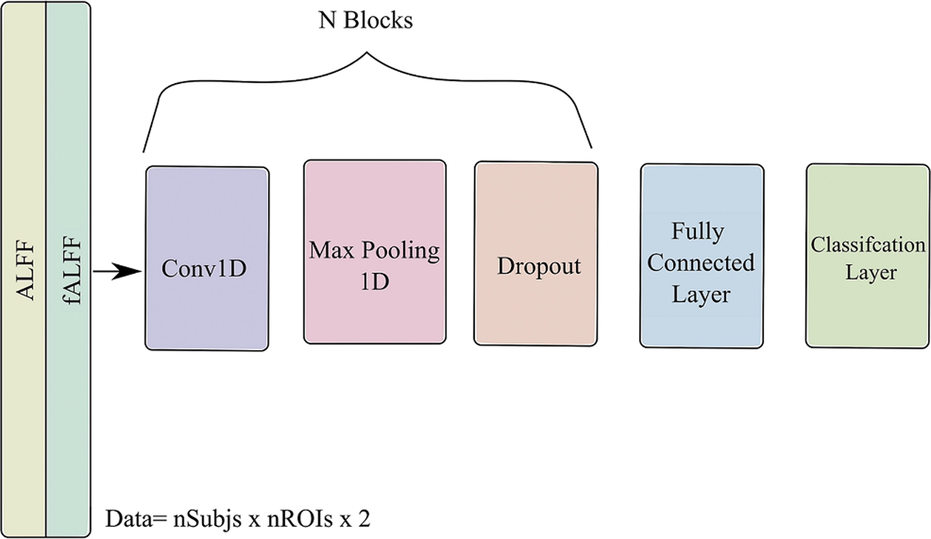
Deep learning architecture for sex classification. The architecture consists of N-block of a stacked convolutional layer, max pooling, and dropout layers. The previous architecture resulted in three models based on N = 1, 2, and 3.

Evaluation strategy

We utilized the area under the curve (AUC) for reporting the results. AUC is less sensitive for imbalanced classes and offers a robust measure for binary classification problems (Ling et al., 2003). Using 10 repeats, the average AUC is adopted to select the best classifier or atlas, which offers better estimation of the distribution of performances. In addition, we used stratified nested cross-validation (sNCV) instead of the classical cross-validation to preserve the ratio of samples between the groups while providing unbiased estimation (Kohavi, 1995; Krstajic et al., 2014). The sNCV avoids biased results by isolating testing data from any parameter optimization. We used an inner loop of threefold cross-validation to optimize each classifier's parameters. Then, the model with the best performance was used to extract the prediction from the testing set. We always report the AUC for the testing set and refer to it as an out-of-sample performance.

We followed three evaluation strategies to evaluate sex classification. First, we assessed the performance of each ML approach on each data set (within-sample evaluation) and reveal the effect of unbalanced data sets on the accuracy of sex classification. Second, we used leave-one-scan-out (across-sample evaluation) to test the reproducibility of predicting sex across different data sets. Third, we focused on HCP to evaluate the effect of scanning time on the predictability of sex. More specifically, we varied the number of samples [32, 150, 300, 600, 900, 1200] and calculated the AUC accordingly. The analysis was applied to both atlases for only the best classifiers found from previous analyses. Finally, we investigated the ICC from the HCP to evaluate the consistency of predictions across HCP scans. ICC measures the amount of variability that can be explained by an objective of measurement, such as subject (Shrout and Fleiss, 1979). We reported the ICC (2,1), which is used to estimate the agreements (predicted probabilities) when the sources of error are known (multiple scans from HCP). To offer an accurate estimation of ICC, we split each scan's data into 50-fold sNCV and estimated the probability of each sample in the testing set. We repeated the probability estimation for all scans using the AAL and Power atlases. It should be noted that only the best ML method found from previous analyses was used to estimate the predicted probability of sex.

Feature importance

To reveal and map the important features for sex classification, while providing interpretable results, we propose using the Shapley Additive (SHAP) approach (Lundberg and Lee, 2017; Lundberg et al., 2020; Štrumbelj and Kononenko, 2014). SHAP deploys a game-theoretical approach to estimate Shapley values (SHV) of a cooperative game while assuming each feature as an independent player. To compute SHV, each feature goes under random sampling and substantiation to assess the impact of those features on the overall prediction. In our analysis, we used the best classifier obtained in the analysis as an Explainer. The process was done in 10-fold cross-validation with 5 repeats. The final SHV were obtained as the average of out-of-sample prediction within each scan. The sign and strength of SHV represent the importance of predicting and the direction of prediction (positive is males and negative in females, based on our class encoding).

Results

First, we investigated the performance of the classical ML and DL in predicting sex across all the five data sets. Figure 2 shows a box plot of the AUC classification performance using classical ML and DL models (10 repeats with 10-fold sNCV).

FIG. 2.

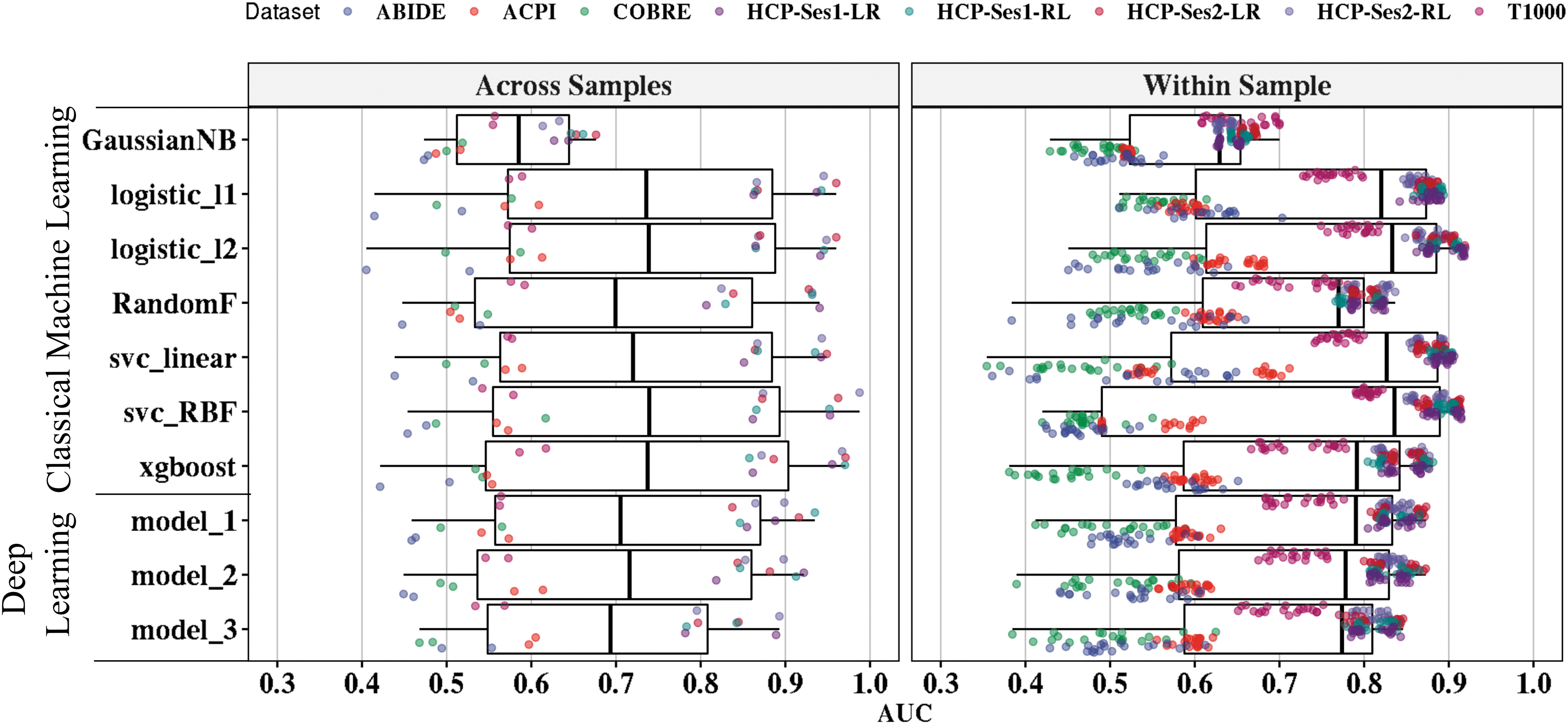
Binary classification performance of individual classifiers from classical ML and DL models. Overall, the figure shows the out-of-sample AUCs for within-sample evaluations (1600 runs) and across-sample evaluations (160 runs). The vertical axis represents tested ML models from classical ML (n = 7) and DL with spatial information (n = 3). The models are ordered as following: (1) Gaussian naive Bayes (GaussianNB), (2) logistic regression with ℓ1-norm (logistic_l1), (3) logistic regression with ℓ2-norm (logisitc_l2), (4) Random Forests Classifier (RandomF), (5) support vector classification with linear kernel (svc_linear), (6) support vector classification with radial basis function (svc_RBF), (7) extreme gradient boosting (XGBoost) algorithms, (8) DL with one-convolutional layer (model_1), DL with two-convolutional layers (model_2), and DL with three-convolutional layers (model_3). The horizontal axis represents the AUC value based on the evaluation procedure, adopted atlas, and the classifier. For across-sample validation (left panel), each point represents the AUC value of the leave-one-scan-out from each classifier tested on features extracted from AAL and Power's atlases (2 atlases × 8 scans = 16 points per classifier). For within sample (right panel), each point is the out-of-sample AUC values after running classifiers on each atlas and each scan with 10 repeats (10 repeats × 10-folds × 2 atlases × 8 scans = 160 per algorithm). For clarity purposes, each point was randomly jittered on the vertical axis. AAL, automated anatomical labeling; AUC, area under the curve; DL, deep learning; ML, machine learning.

Logistic regression methods with ℓ2-norm and ℓ1-norm yielded, on average, the best AUCs of 76% ± 15% and 74.1% ± 13.7%, respectively, for within-sample classification. Other classifiers achieved the following accuracies: svc with linear kernel (74.1% ± 17.3%), svc with RBF kernel (72.9% ± 19%), XGBoost (71.6% ± 15.1%), Random Forest (70.2% ± 11.8%), and Gaussian naive Bayes (59.5% ± 7.3%). Similarly, logistic regression with ℓ2-norm achieved the best accuracy of 72.8% ± 19.4% for across-sample evaluation, followed by XGBoost. Thus, we selected and used logistic regression with ℓ2-norm for our further analysis.

In Figure 3, we show the performance of logistic regression with ℓ2-norm performance on the individual data sets using across- and within-sample evaluation.

FIG. 3.

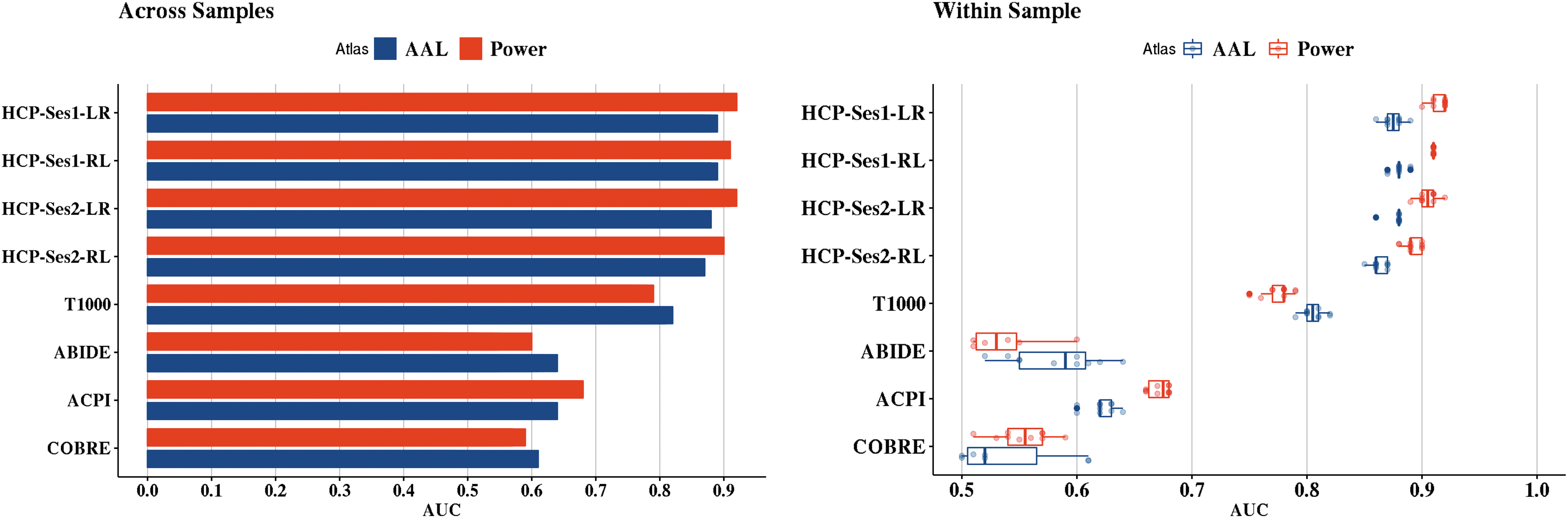
The yielded out-of-sample AUC values using logistic regression with ℓ2-norm based on each atlas. The left panel represents the across-sample evaluation, while the right panel represents the within-sample evaluation from each of the 10 repeats.

We also compared the performance of classifiers based on the adopted atlas (Fig. 4). From the analysis, Power's functional atlas achieved the highest average AUC of 71.8% ± 20% and 71.6% ± 15.6% for across- and within-sample evaluation. AAL achieved 68.2% ± 15.7% for across-sample evaluation and 70.6% ± 14.5% for within-sample evaluation.

FIG. 4.

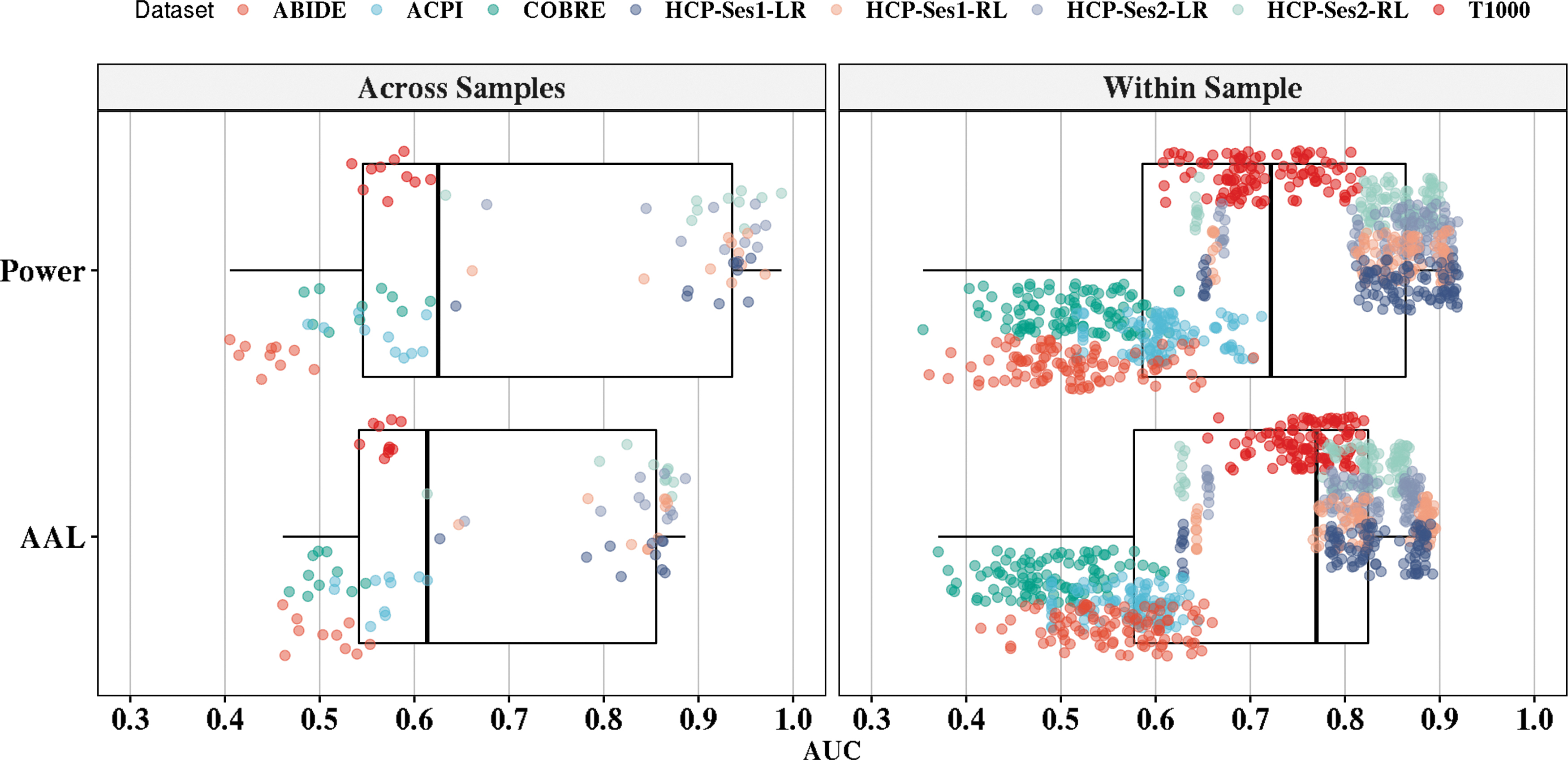
The effect of atlas selection on the performance of sex classification. The vertical axis represents AAL and Power's atlases. The horizontal axis represents the AUC performance of the out-of-sample values. The left panel represents the out-of-sample AUC box plot across all classifiers (10 classifiers × 8 scans = 80 runs per atlas). The right panel depicts the within-sample AUC values across all classifiers (10 repeats × 10-folds × 10 classifiers × 8 scans = 800 runs per atlas). For clarity purposes, each point was randomly jittered on the vertical axis.

The effect of the number of samples on the prediction accuracies is shown in Figure 5. Power's functional atlas performed better than AAL when fixing the number of samples. The accuracy does not seem to improve after 600 to 900 time points for Power's atlas; however, the AAL improves over the number of samples but does not reach Power's atlas performance.

FIG. 5.

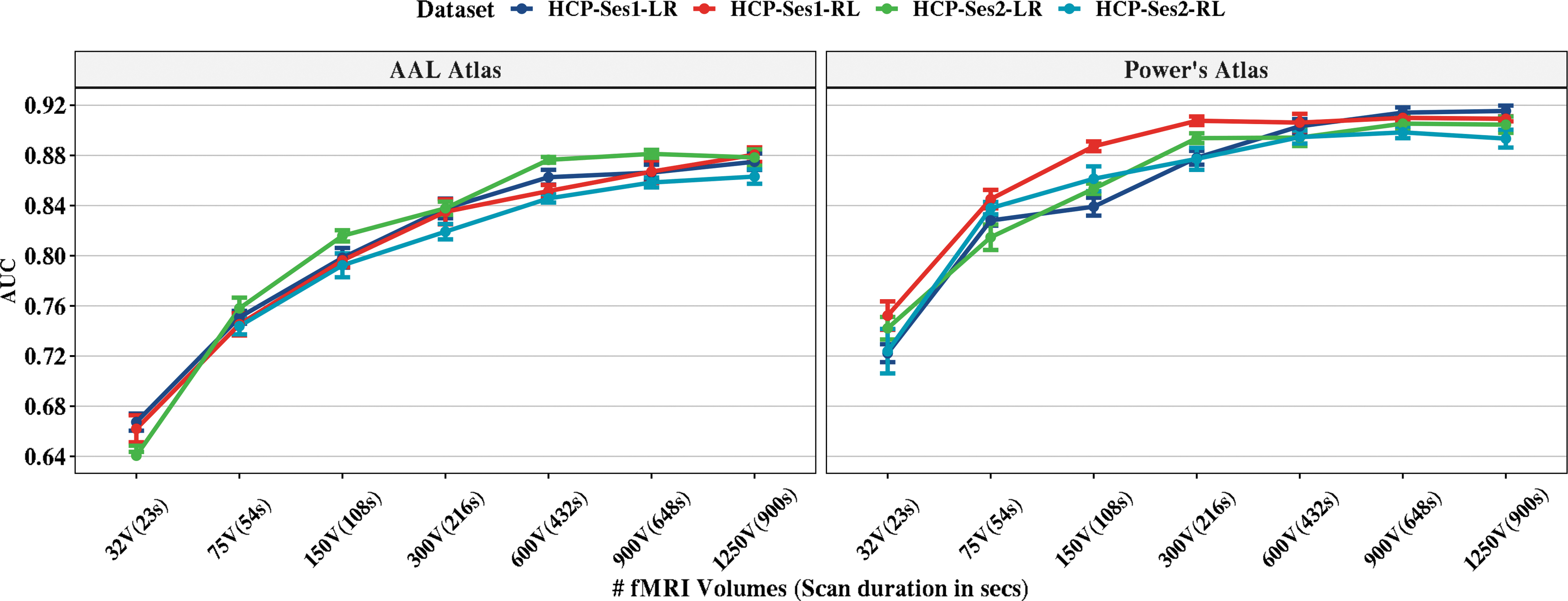
The effect of the number of volumes on sex classification from HCP scans. For each of the number of volumes, we ran 10-repeat of 10-fold sNCV on the data and reported the out-of-sample AUC values using logistic regression with the ℓ2-norm classifier. The left panel represents the AAL atlas performance, and the right panel shows the Power's atlas performance. The error bars represent the standard deviation of AUCs from the 10-repeats (10 repeats × 10-folds). HCP, Human Connectome Project; sNCV, stratified nested cross-validation.

We also assessed the test–retest reliability by calculating the ICC using the four scans of the HCP data set. We used the logistic regression with the ℓ2-norm to estimate the predicted probabilities of sex with sNCV configuration (testing set). As in the previous analyses, we used combined ALFF and fALFF features as an input for the logistic regression with the ℓ2-norm. The results indicated moderate reliability for AAL with ICC = 0.65 [0.63–0.67] and good reliability for Power's atlas with ICC = 0.78 [0.76–0.80].

Feature importance for AAL and Power's atlases is shown in Figures 6 and 7. For Power's ROIs, the size and color of the nodes represent the importance of those nodes in predicting sex from the five data sets. The importance was computed using SHV from logistic regression with the ℓ2-norm explainer. The red color represents the importance of predicting females, while blue represents predicting males. Similarly, we mapped the SHV for AAL on the surface of the brain while using the same color coding in Power's atlas. It should be noted that the SHV were calculated for the out-of-sample prediction and averaged over five repeats. For the AAL atlas with fALFF features, the most important brain regions for predicting females included Cingulum_Post_L, Frontal_Sup_Orb_R, and Caudate_R, while the regions for males included Cerebelum_7b_R, Temporal_Pole_Mid_L, and Cingulum_Ant_R. For ALFF features, the important regions for predicting females included Putamen_L, Temporal_Pole_Mid_L, and Occipital_Sup, while for males, the regions included Cerebelum_10_R, Frontal_Inf_Orb_L, and Olfactory_L. In addition, Power's ROIs showed lower overall importance compared with the AAL atlas. In detail, the important brain networks based on ROI locations for predicting females using fALFF features included subcortical, cerebellar, and dorsal attention networks, while the networks for males were memory retrieval, DMN, and salience network. For the ALFF feature, only the ventral attention network was important for predicting females. Memory retrieval, subcortical, and cerebellar were the important networks for predicting males.

FIG. 6.

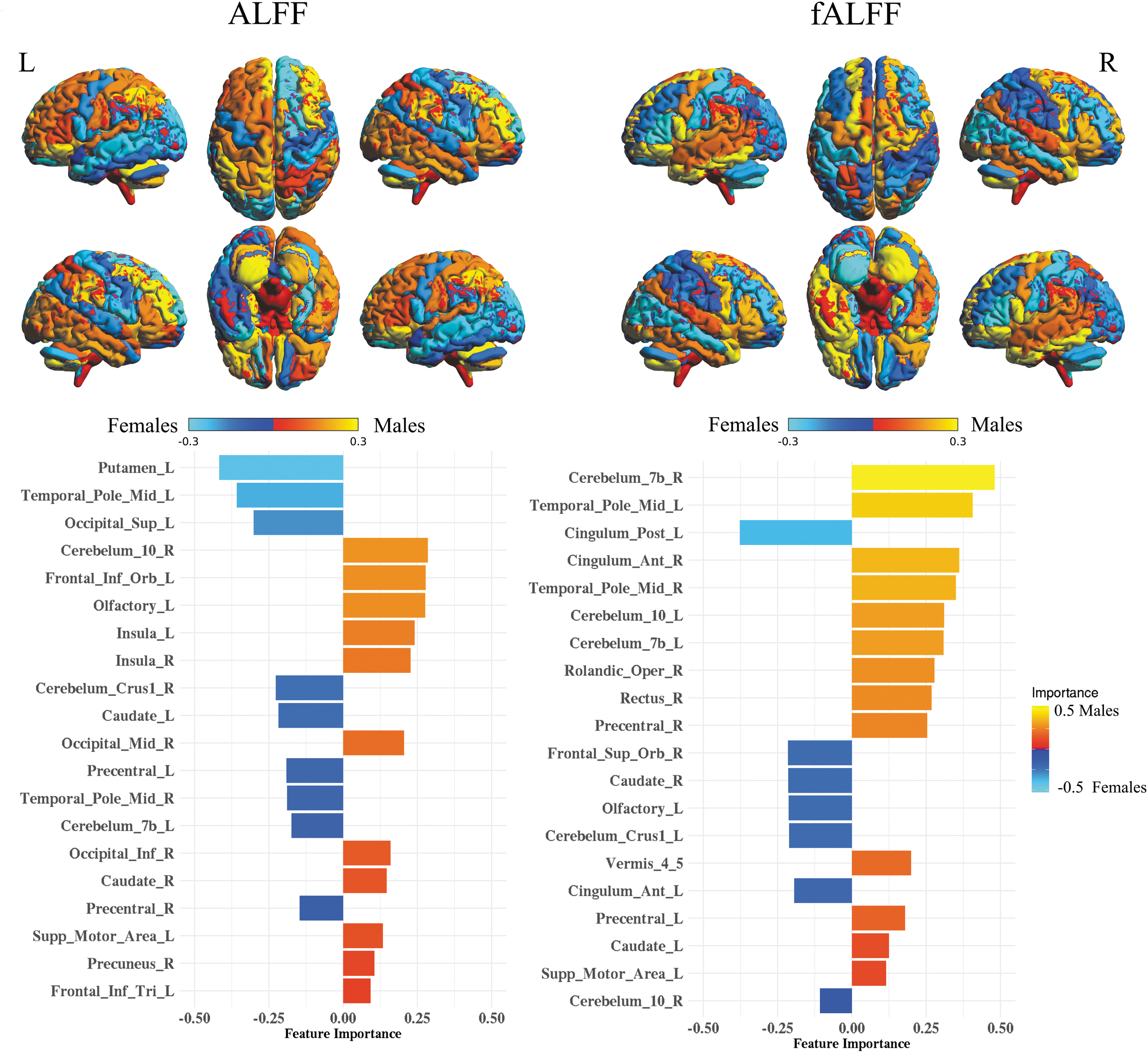
ALFF and fALFF feature maps and importance in sex classification using SHV for AAL atlas. The colors are mapped based on the SHV and reveal the contribution of each region in sex classification. The bar plot shows the top 20 features ordered based on the absolute SHV. ALFF, amplitude of low-frequency fluctuation; fALFF, fraction of ALFF; SHV, shapely values.

FIG. 7.

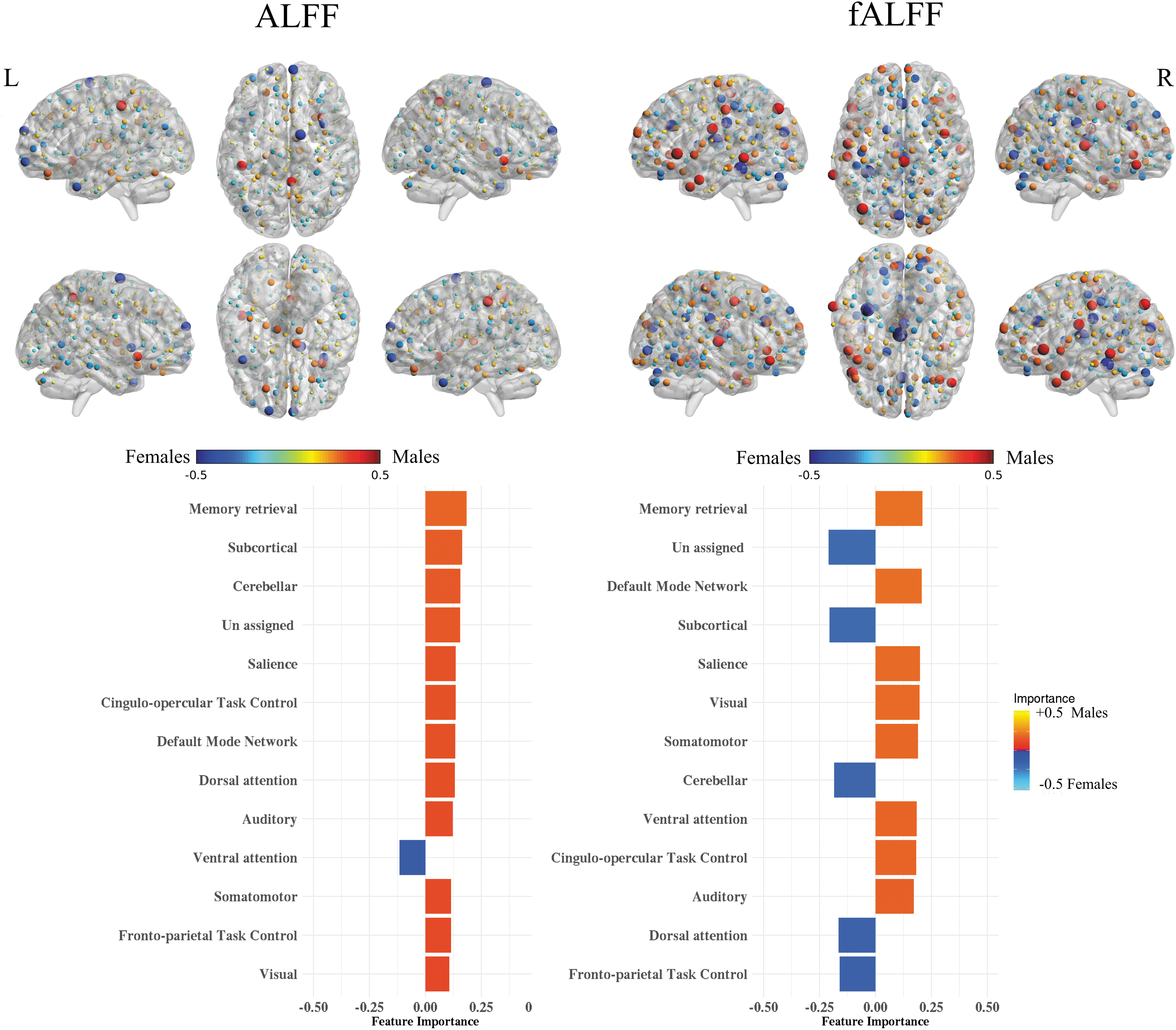
ALFF and fALFF feature maps and importance in sex classification using SHV for Power's functional atlas. The colors are mapped based on the SHV and reveal the contribution of sex classification. For the bar plot, the 264 regions were aggregated based on the assigned brain system (Power et al., 2011) and ordered based on the mean absolute SHV.

Discussion

We conducted comprehensive analyses to predict sex from rsfMRI across five independently acquired data sets and structured the discussion as follows.

Predictability of sex

We show that males and females can be classified with high accuracy in healthy young adults when using intrinsic BOLD fluctuation properties, while deteriorating in heterogenous data sets (Fig. 2). To avoid the “curse of dimensionality,” we focused on the ROI approach to characterize the BOLD fluctuation properties rather than using whole-brain data. This allowed us to have a robust prediction and avoid potential overfitting (Guyon and Elisseeff, 2003; Hua et al., 2009; Mwangi et al., 2014). We derived ROIs from two atlases, namely, Power's functional atlas and the AAL atlas. Both atlases are widely used in analyzing rsfMRI data and manifest different methodologies in parcellating the brain. While Power's atlas uses the functional organizations of the brain, dividing it into 264 ROIs, the AAL atlas relies on the anatomical distribution of the brain, categorizing it into 116 brain regions. Overall, we found that sex is predictable with the highest accuracy in healthy young adults (HCP data set). The more heterogeneous the data set becomes, including the mental illness factor, the less predictable the sex is. Other used data sets varied in population and mixed clinical symptoms, with the best sex prediction performance achieved in the T1000 data set. Our findings support and extend the good sex classification results based on fMRI FC, as shown in Weis and colleagues (2020) and Zhang and colleagues (2018). In addition, it supports the notation that mental illnesses disrupt the properties of BOLD fluctuation as it has been shown in several clinical populations such as autism (Itahashi et al., 2015; Noonan et al., 2009), ADHD (Tang et al., 2018), schizophrenia (Hoptman et al., 2010; Yu et al., 2014), bipolar disorder (Meda et al., 2015; Yang et al., 2019), and depression (Jing et al., 2013). Altogether, the results may suggest that sex difference is primarily encoded in the low-frequency BOLD fluctuations as characterized in the ALFF and fALFF measures and can be potentially used as a biomarker for analyzing different clinical populations.

Effect of classifier on sex predictability

We investigated the choice of the classifier on the performance of sex classification using several classical ML and DL methods. We extensively benchmarked several approaches and showed that several methods could outperform support vector machine (SVM) used in other works (Dhamala et al., 2020; Weis et al., 2020). Although Dhamala and colleagues (2020) and Weis and colleagues (2020) used an SVM classifier for FC data, our works show the need to benchmark other approaches for FC. In addition, the results revealed that linear classifiers outperformed both nonlinear classifiers and DL models with the best average AUC value using logistic regression with ℓ2-norm, followed by logistic regression with ℓ1-norm regularization. The performance of classifiers was evaluated using across and within samples. The performance of predicting sex varied across the data sets and scans, with the best performance using the four scans of HCP—the performance of classification degraded as a function of the heterogeneity of the sample. Thus, BOLD fluctuation properties may be largely impacted by the clinical diagnosis and can thus potentially be biomarkers for clinical symptoms.

Effect of ROI selection

Both atlases yielded close accuracies, with an advantage for Power's atlas. More specifically, Power's atlas achieved a higher average AUC than the AAL atlas for all data sets, except for the T1000 and ABIDE data sets (using l2-nom logistic regression). Similarly, Power's atlas resulted in better AUC for all data sets except for T1000, ABIDE, and COBRE-MIND data sets when using across-sample evaluation. The difference in the performance may be attributed to the disease-specific alteration of structural and functional originations of the brain.

Generalizability

We tested the generalizability of sex classification by using an across-data set evaluation approach; we trained on all scans except one, which was then used for testing—this equivalent of using each testing set as a discovery data set. The analysis resulted in one AUC per data set and atlas. We compared both classical ML and DL to investigate the generalizability of each classifier. The results indicated low generalizability across data sets except for HCP. The fact that HCP comprised multiple scans recorded from the same subjects has contributed to the high AUC within each scan. As in the within-sample evaluation, linear classifiers outperformed nonlinear classifiers with the advantage of ℓ2-norm logistic regression over other classifiers. DL models did not generalize very well, yielding results similar to the nonlinear classical ML methods. Thus, further research should be conducted to find suitable ML techniques for brain imaging data that account for variability across subjects, a limited number of samples, and high-dimensional data. It should be noted that we selected data sets preprocessed with the same pipeline if possible, for example, ABIDE and COBRE data sets used the NIAK pipeline, which will allow for better replication as opposed to reprocessing data with new pipelines. In addition, our validation procedure accounts for preprocessing variations by running within-data set validation (each data set will have the same preprocessing and scanner parameters). In addition, the within-data set validation also tests the effect of the imbalanced distribution of sex for some data sets (e.g., ABIDE and ACPI vs. HCP). More specifically, HCP is a highly balanced data set with a matched preprocessing pipeline. Thus, one can conclude that sex differences can be detected with high accuracy.

The effect of the number of samples

The effect of the number of samples (e.g., resting fMRI scan duration) on sex classification was evaluated on HCP scans since they have the longest scan time (∼15 min). For each scan, we took the first s = [32, 75, 150, 300, 600, 900, 1200] samples and extracted ALFF and fALFF features. Each time, we accessed the AUC for within-sample 10-repeats of 10-fold NCV. Using only the first 32 samples from HCP scans, AUCs were between 0.66 and 0.72. The performance for Power's atlas seems to plateau between 600 and 900 samples with little improvement after adding more samples. The AAL atlas performance was lower than Power's atlas for the same number of points. Thus, researchers should account for sex differences for experiments with even short innervation design (e.g., block design experiments).

Test–retest reliability

The test–rest reliability of sex classification was assessed by calculating the ICCs from HCP scans. The results indicated moderate reliability for AAL with ICC = 0.65 [0.63–0.67] and good reliability for Power's atlas with ICC = 0.78 [0.76–0.80]. The moderate and good reliability from the HCP data set offers promising results for using ML to analyze rs-fMRI instead of the traditional FC analysis of rs-fMRI. The reliability of ALFF and fALFF has been shown across sessions (Zuo et al., 2010a), unlike the reliability of the classical FC analysis of rs-fMRI (Noble et al., 2017, 2019), which led many researchers to endorse the notion of the “reproducibility crisis” for FC (Baker, 2016). Thus, the reliability of low-frequency fluctuation properties across sessions, along with moderate to good prediction reliability, makes them better measures to study and characterize brain functional responses in health and disease.

Spatial distribution and feature importance

We adopted the SHAP approach to assessing feature importance and directionality in predicting each sex. For AAL atlas, we mapped the SHAP values on the surface of the brain. The results revealed that sex classification is not associated with one specific region but varies across the brain and subfeature sets. Also, there are no regions that are associated explicitly with differentiating females from males. However, some brain regions are consistently among the top important parts in predicting sex, such as the cerebellum and temporal pole for ALFF and fALFF. Top features in our case span over part of the DMN, temporal pole, precuneus, and insular cortex regions. In addition, we observed an overlap for top brain regions differentiating sex—in our case sex difference analysis using GMV analysis (Liu et al., 2020) and FC analysis (Weis et al., 2020). Also, we replicated the observation that the DMN is one of the top features in differentiating sex, in line with the findings from Biswal and colleagues (2010) and Zhang and colleagues (2018).

For the Power's functional atlas, we plotted the top features using node size and color. Some ROIs overlap with top important features from the AAL, such as in the DMN and temporal pole. We reported average SHAP values by averaging them by the brain system (Power et al., 2011) and showed that brain regions involved in memory retrieval constitute the top predicting features in both ALFF and fALFF features (Fig. 7). Overall, the obtained distribution of feature importance supports the notion that the brain consists of mosaic features (Joel and Fausto-Sterling, 2016; Joel et al., 2015; Shalev et al., 2020), where some features are more pronounced in one sex than in the other. In our case, the mosaic features are not only spatially distributed but also span across ALFF and fALFF features.

Sex consideration in analyzing rs-fMRI

Our results showed strong evidence that sex differences influence BOLD fluctuation properties and potentially confound the influence of other neurobiological factors, which may broadly impact the interpretation of rs-fMRI results. Also, our analysis revealed an interaction between mental disorders, sex, and BOLD fluctuations. Thus, our analyses strongly suggest that the sex variable should be accounted for (e.g., using sex as a covariate) in analyzing and interpreting rs-fMRI and potentially task-based fMRI. In addition, other sex-based biological factors should be considered in the analysis, such as the menstrual cycle, as it has been shown to affect rs-fMRI signal (Hjelmervik et al., 2014; Weis et al., 2019).

Beyond sex classification

The same framework utilized in this work can be used to classify and predict other outcomes such as clinical scales, diagnoses, and cognitive performance from rs-fMRI. Other atlas and ML methods can be included in the framework accordingly.

Limitations

In this work, we explored using rs-fMRI to predict sex from five independent data sets. The data sets were collected at various sites using different MRI scanners, populations, preprocessing pipelines, and other configurations. The effect of these factors on predicting sex is still not apparent nor well characterized (Botvinik-Nezer et al., 2020). In addition, other factors can contribute to sex differences in the brain, such as disease state (Cahill, 2014), and other biological factors such as the menstrual cycle (Hjelmervik et al., 2014; Weis et al., 2019). In addition, we used two the AAL atlas and Power's atlas only. There are many other functional and anatomical atlases that can be adopted. We used several ML and DL methods, but there are many other ML methods and DL architectures that have not been explored here. We used ALFF and fALFF for describing BOLD signal fluctuations; however, other features can be defined and used.

Conclusion

ML has gained popularity in predicting different outcomes in human brain neuroimaging data. In this work, we have shown that sex can be predicted with high accuracy from rs-fMRI using various classical ML and DL approaches. We adopted unbiased and explainable methods in our framework with comprehensive validation procedures. The results demonstrated that sex difference is embedded in the properties of low-frequency BOLD signal fluctuation and extends the previous findings of sex difference reported based on fMRI FC. We assessed the sex classification of five different and independent data sets that vary in population, including healthy young adults to other clinical populations. The highest archived results occurred when using healthy young adults only and may reflect the effect of the mental illnesses on the properties of the BOLD signal. The best classification performance was obtained with the use of linear classifiers, and we did not find an advantage of using DL methods. The spatial distribution of the important features was consistent with the previous finding, but we showed that sex classification did not rely on a specific brain region or on one subfeature set. It should be noted that we matched the preprocessing pipelines as much as possible. The results presented here suggest that sex distribution should be seriously considered in any brain imaging study, including studies that investigate FC, BOLD activation, or structural analyses.

Footnotes

Acknowledgments

We thank “Tulsa 1000 Investigators,” including Drs. Robin Aupperle, Justin Feinstein, Sahib S. Khalsa, Rayus Kuplicki, Jonathan Savitz, Jennifer Stewart, and Teresa A. Victor for helping in this work. We also thank the open-source data community and preprocessed data initiatives for giving access to rest-fMRI data sets and funding agencies. The funding and support for each data set are as follows: (1) ACPI is primarily supported by a grant supplement (R01 MH094639) by the National Institute on Drug Abuse (NIDA). Additional support was provided by the Child Mind Institute and the Nathan Kline Institute; (2) ABIDE: the Autism Brain Imaging Data Exchange for preprocessing and providing the data; (3) COBRE-MIND: the National Institute of Health Center of Biomedical Research Excellence grant 1P20RR021938-01A2; (4) HCP: data were provided [in part] by the Human Connectome Project, WU-Minn Consortium (Principal Investigators: David Van Essen and Kamil Ugurbil; 1U54MH091657) funded by the 16 NIH Institutes and Centers that support the NIH Blueprint for Neuroscience Research; and by the McDonnell Center for Systems Neuroscience at Washington University.

Authors' Contributions

O.A.Z. suggested the analysis to J.B.; J.B. evaluated and assigned the study to O.A.Z.; O.A.Z. and J.B. developed the study design, and J.B. acquired the financial support for the project; O.A.Z., M.M., A.T., V.Z., J.B., and T1000 developed and facilitated data collection and the infrastructure for conducting data analyses; O.A.Z., M.M., and J.B. developed data analysis pipelines; O.A.Z. developed the machine learning pipeline; O.A.Z. wrote the original article draft; O.A.Z., E.W., V.Z., M.M., M.P.P., and T1000 provided guidance on analyses and critical review of the article; all authors provided comments.

Availability of Data and Code

Support for the findings and scripts of this study are available from the corresponding author upon reasonable request. Public data sets used here (except for T1000) are available through the corresponding data holders and should be requested accordingly.

Codes will be available upon request from the corresponding author.

Author Disclosure Statement

No competing financial interests exist.

Funding Information

This work has been supported directly by The William K. Warren Foundation, Laureate Institute for Brain Research, and, in part, by the P20 GM121312 award from the National Institute of General Medical Sciences, National Institutes of Health.

References

Al Zoubi

, Awad

, Kasabov

. 2018a. Anytime multipurpose emotion recognition from EEG data using a Liquid State Machine based framework. Artif Intell Med, 86:1–8.

Al Zoubi

, Ki Wong

, Kuplicki

, et al. 2018b. Predicting age from brain EEG signals—a machine learning approach. Front Aging Neurosc, 10:184.

Al Zoubi

, Misaki

, Tsuchiyagaito

, et al. 2020. Predicting sex from resting-state fMRI across multiple independent acquired datasets. bioRxiv, 2020. DOI: 10.1101/2020.08.20.259945.

Allen

, Erhardt

, Damaraju

, et al. 2011. A baseline for the multivariate comparison of resting-state networks. Front Syst Neurosci, 5:2.

Alonso-Solís

, Vives-Gilabert

, Portella

, et al. 2017. Altered amplitude of low frequency fluctuations in schizophrenia patients with persistent auditory verbal hallucinations. Schizophr Res, 189:97–103.

Bai

, Liao

, Watson

, et al. 2011. Mapping the altered patterns of cerebellar resting-state function in longitudinal amnestic mild cognitive impairment patients. J Alzheimers Dis, 23:87–99.

Baker

2016. 1,500 scientists lift the lid on reproducibility. Nature, 533:452–454.

Bellec

, Lavoie-Courchesne

, Dickinson

, et al. 2012. The pipeline system for Octave and Matlab (PSOM): a lightweight scripting framework and execution engine for scientific workflows. Front Neuroinform, 6:7.

Besson

, Magne

, Schön

. 2002. Emotional prosody: sex differences in sensitivity to speech melody. Trends Cogn Sci, 6:405–407.

10.

Biswal

BB.

2012. Resting state fMRI: a personal history. Neuroimage, 62:938–944.

11.

Biswal

, Mennes

, Zuo

X-N

, et al. 2010. Toward discovery science of human brain function. Proc Natl Acad Sci U S A, 107:4734–4739.

12.

Bluhm

, Osuch

, Lanius

, et al. 2008. Default mode network connectivity: effects of age, sex, and analytic approach. Neuroreport, 19:887–891.

13.

Botvinik-Nezer

, Holzmeister

, Camerer

, et al. 2020. Variability in the analysis of a single neuroimaging dataset by many teams. Nature, 582:84–88.

14.

Cahill

2014. Fundamental sex difference in human brain architecture. Proc Natl Acad Sci U S A, 111:577–578.

15.

Calhoun

, Sui

, Kiehl

, et al. 2012. Exploring the psychosis functional connectome: aberrant intrinsic networks in schizophrenia and bipolar disorder. Front Psychiatry, 2:75.

16.

Campbell

, Huang

, Zhang

, et al. 2020. Pharmacologically informed machine learning approach for identifying pathological states of unconsciousness via resting-state fMRI. Neuroimage, 206:116316.

17.

Chekroud

, Ward

, Rosenberg

, et al. 2016. Patterns in the human brain mosaic discriminate males from females. Proc Natl Acad Sci U S A, 113:E1968.

18.

Chen

, Guestrin

Xgboost: a scalable tree boosting system. In Paper Presented at the Proceedings of the 22nd ACM SIGKDD International Conference on Knowledge Discovery and Data Mining, Association for Computing Machinery, San Francisco, CA, USA, 2016.

19.

Cohen

, Chen

, Parker Jones

, et al. 2020. Regression-based machine-learning approaches to predict task activation using resting-state fMRI. Hum Brain Mapp, 41:815–826.

20.

Cordes

, Haughton

, Arfanakis

, et al. 2001. Frequencies contributing to functional connectivity in the cerebral cortex in “resting-state” data. Am JNeuroradiol, 22:1326–1333.

21.

Craddock

, Benhajali

, Chu

, et al. 2013. The neuro bureau preprocessing initiative: open sharing of preprocessed neuroimaging data and derivatives. Neuroinformatics, 41. DOI: 10.3389/conf.fninf.2013.09.00041.

22.

Damoiseaux

, Rombouts

, Barkhof

, et al. 2006. Consistent resting-state networks across healthy subjects. Proc Natl Acad Sci U S A, 103:13848–13853.

23.

Del Giudice

2009. On the real magnitude of psychological sex differences. Evol Psychol, 7:147470490900700209.

24.

Del Giudice

, Lippa

, Puts

, et al. 2016. Joel et al.'s method systematically fails to detect large, consistent sex differences. Proc Natl Acad Sci U S A 113:E1965.

25.

Dhamala

, Jamison

, Sabuncu

, et al. 2020. Sex classification using long-range temporal dependence of resting-state functional MRI time series. Hum Brain Mapp, 41:3567–3579.

26.

Di Martino

, Yan

C-G

, Li

, et al. 2014. The autism brain imaging data exchange: towards a large-scale evaluation of the intrinsic brain architecture in autism. Mol Psychiatry, 19:659–667.

27.

, Fu

, Calhoun

. 2018. Classification and prediction of brain disorders using functional connectivity: promising but challenging. Front Neurosci, 12:525.

28.

Elliott

, Sharp

, Alfaro-Almagro

, et al. 2018. Genome-wide association studies of brain imaging phenotypes in UK Biobank. Nature, 562:210–216.

29.

Feis

D-L

, Brodersen

, von Cramon

, et al. 2013. Decoding gender dimorphism of the human brain using multimodal anatomical and diffusion MRI data. Neuroimage, 70:250–257.

30.

Fox

, Snyder

, Vincent

, et al. 2007. Intrinsic fluctuations within cortical systems account for intertrial variability in human behavior. Neuron, 56:171–184.

31.

Garner

, La Rocca

, Barisano

, et al. A machine learning model to predict seizure susceptibility from resting-state fMRI connectivity. In Paper Presented at the 2019 Spring Simulation Conference (SpringSim). IEEE, 2019, pp. 1–11.

32.

Glover

, Li

, Ress

. 2000. Image-based method for retrospective correction of physiological motion effects in fMRI: RETROICOR. Magn Reson Med, 44:162–167.

33.

Guyon

, Elisseeff

. 2003. An introduction to variable and feature selection. J Mach Learn Res, 3:1157–1182.

34.

, Kong

, Holmes

, et al. 2020. Deep neural networks and kernel regression achieve comparable accuracies for functional connectivity prediction of behavior and demographics. Neuroimage, 206:116276.

35.

Hjelmervik

, Hausmann

, Osnes

, et al. 2014. Resting states are resting traits—an FMRI study of sex differences and menstrual cycle effects in resting state cognitive control networks. PLoS One, 9:e103492.

36.

Hoptman

, Zuo

X-N

, Butler

, et al. 2010. Amplitude of low-frequency oscillations in schizophrenia: a resting state fMRI study. Schizophr Res, 117:13–20.

37.

Hua

, Tembe

, Dougherty

. 2009. Performance of feature-selection methods in the classification of high-dimension data. Pattern Recognit, 42:409–424.

38.

Hyde

, Plant

. 1995. Magnitude of psychological gender differences: another side to the story. Am Psychol, 50:159–161.

39.

Ingalhalikar

, Smith

, Parker

, et al. 2014. Sex differences in the structural connectome of the human brain. Proc Natl Acad Sci U S A, 111:823–828.

40.

Itahashi

, Yamada

, Watanabe

, et al. 2015. Alterations of local spontaneous brain activity and connectivity in adults with high-functioning autism spectrum disorder. Mol Autism, 6:30.

41.

Jing

, Liu

C-H

, Ma

, et al. 2013. Difference in amplitude of low-frequency fluctuation between currently depressed and remitted females with major depressive disorder. Brain Res, 1540:74–83.

42.

, Saad

, Simmons

, et al. 2010. Mapping sources of correlation in resting state fMRI, with artifact detection and removal. Neuroimage, 52:571–582.

43.

Joel

, Berman

, Tavor

, et al. 2015. Sex beyond the genitalia: the human brain mosaic. Proc Natl Acad Sci U S A, 112:15468–15473.

44.

Joel

, Fausto-Sterling

. 2016. Beyond sex differences: new approaches for thinking about variation in brain structure and function. Philos Trans R S B Biol Sci, 371:20150451.

45.

Kazeminejad

, Sotero

. 2019. Topological properties of resting-state fMRI functional networks improve machine learning-based autism classification. Front Neurosci, 12:1018.

46.

Kohavi

A study of cross-validation and bootstrap for accuracy estimation and model selection. In Paper Presented at the Ijcai. Montreal, Quebec: Morgan Kaufmann Publishers Inc., 20 August, 1995.

47.

Krstajic

, Buturovic

, Leahy

, et al. 2014. Cross-validation pitfalls when selecting and assessing regression and classification models. J Cheminform, 6:1–15.

48.

Ktena

, Parisot

, Ferrante

, et al. 2018. Metric learning with spectral graph convolutions on brain connectivity networks. Neuroimage, 169:431–442.

49.

, Jing

, Liu

, et al. 2017. Frequency-dependent changes in the amplitude of low-frequency fluctuations in mild cognitive impairment with mild depression. J Alzheimers Dis, 58:1175–1187.

50.

Ling

, Huang

, Zhang

AUC: a statistically consistent and more discriminating measure than accuracy. In Paper Presented at the Ijcai. Acapulco: Morgan Kaufmann, August 9–15, 2003.

51.

Liu

, Seidlitz

, Blumenthal

, et al. 2020. Integrative structural, functional, and transcriptomic analyses of sex-biased brain organization in humans. Proc Natl Acad Sci U S A, 117:18788–18798.

52.

Lundberg

, Erion

, Chen

, et al. 2020. From local explanations to global understanding with explainable AI for trees. Nat Mach Intell, 2:56–67.

53.

Lundberg

, Lee

S-I

. A unified approach to interpreting model predictions. In Paper Presented at the Advances in Neural Information Processing Systems. California: Curran Associates Inc., 2017.

54.

Lurie

, Sikka

, Khanuja

, et al. The configurable pipeline for the analysis of connectomes (C-PAC). In Journal of Cognitive Neuroscience. 55 Hayward Street, Cambridge, MA: MIT Press, 2013, pp. 231–231.

55.

Mantini

, Perrucci

, Del Gratta

, et al. 2007. Electrophysiological signatures of resting state networks in the human brain. Proc Natl Acad Sci U S A, 104:13170–13175.

56.

Mayer

, Ruhl

, Merideth

, et al. 2013. Functional imaging of the hemodynamic sensory gating response in schizophrenia. Hum Brain Mapp, 34:2302–2312.

57.

Meda

, Wang

, Ivleva

, et al. 2015. Frequency-specific neural signatures of spontaneous low-frequency resting state fluctuations in psychosis: evidence from bipolar-schizophrenia network on intermediate phenotypes (B-SNIP) consortium. Schizophr Bull, 41:1336–1348.

58.

Mennes

, Zuo

X-N

, Kelly

, et al. 2011. Linking inter-individual differences in neural activation and behavior to intrinsic brain dynamics. Neuroimage, 54:2950–2959.

59.

Miller

, Halpern

. 2014. The new science of cognitive sex differences. Trends Cogn Sci, 18:37–45.

60.

Mwangi

, Tian

, Soares

. 2014. A review of feature reduction techniques in neuroimaging. Neuroinformatics, 12:229–244.

61.

Nguyen

, Sun

, Alexander

, et al. Modeling Alzheimer's disease progression using deep recurrent neural networks. In Paper Presented at the 2018 International Workshop on Pattern Recognition in Neuroimaging (PRNI). IEEE, 2018, pp. 1–4.

62.

Noble

, Scheinost

, Constable

. 2019. A decade of test-retest reliability of functional connectivity: a systematic review and meta-analysis. Neuroimage, 203:116157.

63.

Noble

, Spann

, Tokoglu

, et al. 2017. Influences on the test–retest reliability of functional connectivity MRI and its relationship with behavioral utility. Cereb Cortex, 27:5415–5429.

64.

Noonan

, Haist

, Müller

R-A

. 2009. Aberrant functional connectivity in autism: evidence from low-frequency BOLD signal fluctuations. Brain Res, 1262:48–63.

65.

Pedregosa

, Varoquaux

, Gramfort

, et al. 2011. Scikit-learn: machine learning in Python. J Mach Learn Res, 12:2825–2830.

66.

Pereira

, Pinto

, Alves

, et al. 2016. Brain tumor segmentation using convolutional neural networks in MRI images. IEEE Trans Med Imaging, 35:1240–1251.

67.

Plis

, Hjelm

, Salakhutdinov

, et al. 2014. Deep learning for neuroimaging: a validation study. Front Neurosci, 8:229.

68.

Power

, Cohen

, Nelson

, et al. 2011. Functional network organization of the human brain. Neuron, 72:665–678.

69.

Rosenblatt

JD.

2016. Multivariate revisit to “sex beyond the genitalia.” Proc Natl Acad Sci U S A, 113:E1966–E1967.

70.

Ruigrok

, Salimi-Khorshidi

, Lai

M-C

, et al. 2014. A meta-analysis of sex differences in human brain structure. Neurosci Biobehav Rev, 39:34–50.

71.

Russell

, Tchanturia

, Rahman

, et al. 2007. Sex differences in theory of mind: a male advantage on Happé's “cartoon” task. Cogn Emot, 21:1554–1564.

72.

Saccà

, Sarica

, Novellino

, et al. 2019. Evaluation of machine learning algorithms performance for the prediction of early multiple sclerosis from resting-state FMRI connectivity data. Brain Imaging Behav, 13:1103–1114.

73.

Schirmer

, Kotz

, Friederici

. 2005a. On the role of attention for the processing of emotions in speech: sex differences revisited. Cogn Brain Res, 24:442–452.

74.

Schirmer

, Striano

, Friederici

. 2005b. Sex differences in the preattentive processing of vocal emotional expressions. Neuroreport, 16:635–639.

75.

Shalev

, Admon

, Berman

, et al. 2020. A mosaic of sex-related structural changes in the human brain following exposure to real-life stress. Brain Struct Funct, 225:461–466.

76.

Shrout

, Fleiss

. 1979. Intraclass correlations: uses in assessing rater reliability. Psychol Bull, 86:420.

77.

Smith

, Douaud

, Chen

, et al. 2021. An expanded set of genome-wide association studies of brain imaging phenotypes in UK Biobank. Nat Neurosci, 24:737–745.

78.

Smith

, Vidaurre

, Beckmann

, et al. 2013. Functional connectomics from resting-state fMRI. Trends Cogn Sci, 17:666–682.

79.

Štrumbelj

, Kononenko

. 2014. Explaining prediction models and individual predictions with feature contributions. Knowl Inf Syst, 41:647–665.

80.

Tang

, Wei

, Zhao

, et al. 2018. Different developmental pattern of brain activities in ADHD: a study of resting-state fMRI. Developmental Neuroscience, 40:246–257.

81.

Tian

, Wang

, Yan

, et al. 2011. Hemisphere-and gender-related differences in small-world brain networks: a resting-state functional MRI study. Neuroimage, 54:191–202.

82.

Tzourio-Mazoyer

, Landeau

, Papathanassiou

, et al. 2002. Automated anatomical labeling of activations in SPM using a macroscopic anatomical parcellation of the MNI MRI single-subject brain. Neuroimage, 15:273–289.

83.

van der Burgh

, Schmidt

, Westeneng

H-J

, et al. 2017. Deep learning predictions of survival based on MRI in amyotrophic lateral sclerosis. Neuroimage Clin, 13:361–369.

84.

Van Essen

, Smith

, Barch

, et al. 2013. The WU-Minn human connectome project: an overview. Neuroimage, 80:62–79.

85.

Van Essen

, Ugurbil

, Auerbach

, et al. 2012. The Human Connectome Project: a data acquisition perspective. Neuroimage, 62:2222–2231.

86.

Victor

, Khalsa

, Simmons

, et al. 2018. Tulsa 1000: a naturalistic study protocol for multilevel assessment and outcome prediction in a large psychiatric sample. BMJ Open, 8:e016620.

87.

Vieira

, Pinaya

, Mechelli

. 2017. Using deep learning to investigate the neuroimaging correlates of psychiatric and neurological disorders: methods and applications. Neurosci Biobehav Rev, 74:58–75.

88.

Wallentin

2009. Putative sex differences in verbal abilities and language cortex: a critical review. Brain Lang, 108:175–183.

89.

Wang

, Dai

, Su

, et al. 2012. Amplitude of low-frequency oscillations in first-episode, treatment-naive patients with major depressive disorder: a resting-state functional MRI study. PLoS One, 7:e48658.

90.

Weis

, Hodgetts

, Hausmann

. 2019. Sex differences and menstrual cycle effects in cognitive and sensory resting state networks. Brain Cogn, 131:66–73.

91.

Weis

, Patil

, Hoffstaedter

, et al. 2020. Sex classification by resting state brain connectivity. Cereb Cortex, 30:824–835.

92.

Weissman-Fogel

, Moayedi

, Taylor

, et al. 2010. Cognitive and default-mode resting state networks: do male and female brains “rest” differently?. Hum Brain Mapp, 31:1713–1726.

93.

, Moeller

, Auerbach

, et al. 2013. Evaluation of slice accelerations using multiband echo planar imaging at 3 T. Neuroimage, 83:991–1001.

94.

Yang

, Liu

, Jiang

, et al. 2019. Common and specific functional activity features in schizophrenia, major depressive disorder, and bipolar disorder. Front Psychiatry, 10:52.

95.

Yu-Feng

, Yong

, Chao-Zhe

, et al. 2007. Altered baseline brain activity in children with ADHD revealed by resting-state functional MRI. Brain Dev, 29:83–91.

96.

, Chien

, Wang

HLS

, et al. 2014. Frequency-specific alternations in the amplitude of low-frequency fluctuations in schizophrenia. Hum Brain Mapp, 35:627–637.

97.

Zhan

, Gao

, Zhou

, et al. 2016. Amplitude of low-frequency fluctuations in multiple-frequency bands in acute mild traumatic brain injury. Front Hum Neurosci, 10:27.

98.

Zhang

, Dougherty

, Baum

, et al. 2018. Functional connectivity predicts gender: evidence for gender differences in resting brain connectivity. Hum Brain Mapp, 39:1765–1776.

99.

Zou

, Ross

, Gu

, et al. 2013. Intrinsic resting-state activity predicts working memory brain activation and behavioral performance. Hum Brain Mapp, 34:3204–3215.

100.

Zou

Q-H

, Zhu

C-Z

, Yang

, et al. 2008. An improved approach to detection of amplitude of low-frequency fluctuation (ALFF) for resting-state fMRI: fractional ALFF. J Neurosci Methods, 172:137–141.

101.

Zuo

X-N

, Di Martino

, Kelly

, et al. 2010a. The oscillating brain: complex and reliable. Neuroimage, 49:1432–1445.

102.

Zuo

X-N

, Kelly

, Di Martino

, et al. 2010b. Growing together and growing apart: regional and sex differences in the lifespan developmental trajectories of functional homotopy. J Neurosci, 30:15034–15043.