
Abstract
Introduction:
Hidden Markov models (HMMs) are a popular choice to extract and examine recurring patterns of activity or functional connectivity in neuroimaging data, both in terms of spatial patterns and their temporal progression. Although many diverse HMMs have been applied to neuroimaging data, most have defined states based on activity levels (intensity-based [IB] states) rather than patterns of functional connectivity between brain areas (connectivity-based states), which is problematic if we want to understand connectivity dynamics: IB states are unlikely to provide comprehensive information about dynamic connectivity patterns.
Methods:
We addressed this problem by introducing a new HMM that defines states based on full functional connectivity (FFC) profiles among brain regions. We empirically explored the behavior of this new model in comparison to existing approaches based on IB or summed functional connectivity states using the Human Connectome Project unrelated 100 functional magnetic resonance imaging “resting-state” dataset.
Results:
Our FFC model discovered connectivity states with more distinguishable (i.e., unique and separable from each other) patterns than previous approaches, and recovered simulated connectivity-based states more faithfully than the other models tested.
Discussion:
Thus, if our goal is to extract and interpret connectivity states in neuroimaging data, our new model outperforms previous methods, which miss crucial information about the evolution of functional connectivity in the brain.
Impact statement
Hidden Markov models (HMMs) can be used to investigate brain states noninvasively. Previous models “recover” connectivity from intensity-based hidden states, or from connectivity “summed” across nodes. In this study, we introduce a novel connectivity-based HMM and show how it can reveal true connectivity hidden states under minimal assumptions.
Introduction
The brain is a dynamical system of interacting and interchanging brain states (Chen et al, 2016; Lurie et al, 2020; Stevner et al, 2019; Vidaurre et al, 2017): patterns of activity levels or connectivity strengths that characterize and quantify network interactions. When extracted from functional magnetic resonance imaging (fMRI) data, these states can be categorized into two groups, defined either by activity levels of one or more nodes (brain areas; intensity-based [IB] states), or by patterns of functional connectivity between nodes (connectivity-based states). In contrast to IB methods, connectivity-based states and their dynamics remain relatively underexplored. Developing and benchmarking new methods for extracting and characterizing these states are therefore of critical importance.
One promising approach used to characterize evolution of IB brain states across time (i.e., not functional connectivity per se) is hidden Markov models (HMMs). HMMs utilize probabilistic methods to determine a hidden state sequence path not directly observable in data (Eddy, 2004; Eddy, 1996; Jurafsky and Martin, 2009; Rabiner, 1989) by inferring underlying IB states, where the probability of residing in any one of these states depends only on the previous state (Eddy, 2004; Eddy, 1996; Rabiner, 1989).
These models are powerful because (1) they have no assumption about relationships among brain states (Chen et al, 2016), and (2) spatial and temporal information are inherent to the model. Because of these properties, HMMs have been used to identify latent brain states through signals acquired from fMRI and magnetoencephalography (Baker et al, 2014; Chen et al, 2016; Eavani et al, 2013; Stevner et al, 2019; Vidaurre et al, 2018a, Vidaurre et al, 2018b; Vidaurre et al, 2017; Vidaurre et al, 2016).
However, what about connectivity-based states? Outside state-based analysis, a common approach is to calculate pairwise dynamic functional connectivity (dFC), that is, the correlation in activity between pairs of nodes in a brain network and how such correlations change across time using a “sliding window” approach (Chen et al, 2016; Lurie et al, 2020; Vidaurre et al, 2017). However, to study connectivity-based states and their evolution, several groups have examined covariance values extracted from IB HMMs, transforming them into Pearson correlations to create connectivity-like states (Chen et al, 2016; Stevner et al, 2019; Vidaurre et al, 2018; Vidaurre et al, 2017).
However, it is unclear to what extent such transformed covariances reflect true underlying connectivity-based states rather than simply the connectivities that the IB states happened to exhibit. Other groups have used principal component analysis (PCA)-based approaches (Vidaurre, 2021; Vidaurre et al, 2021), or those that assume stationarity of intensity across time (Vidaurre et al, 2018a), with varying success. However, a more direct approach seems desirable—one which uses functional connectivity instead of signal intensity as a direct model input.
A more direct approach was recently undertaken by Ou et al (2015), who summed the results from a dFC sliding window analysis into a representative “connectivity vector”—describing a given node's total connectivity to all other nodes in the network—for every time point, and then fitted these with an HMM. Critically, however, this method sums over dynamic changes in pairwise connectivity, thereby potentially obscuring important changes in pairwise connectivities. For example, increased connectivity between the source node and one target node might be balanced by decreased connectivity to another node, such that no change is observed in overall connectivity.
Importantly, interpretation of the output of a fitted HMM depends strongly on the inputs and assumptions used to develop the model, so the states resulting from Ou and colleagues' (2015) method may differ from states recovered by a model fitted to all pairwise correlation values—between all pairs of nodes—within a sliding window.
In this study, we tackled these concerns by evaluating a new HMM-based method that fits all correlation values obtained from a dFC sliding window analysis. We comprehensively compared this novel full functional connectivity HMM (FFC HMM) to two previously reported methods used to examine functional connectivity states in neuroimaging data: (1) a standard IB HMM (Chen et al, 2016; Stevner et al, 2019; Vidaurre et al, 2017) and (2) a summed functional connectivity HMM (SFC HMM) (Ou et al, 2015). We fitted each model to a widely available existing dataset, the Human Connectome Project (HCP) Unrelated 100 (Van Essen et al, 2013) resting-state fMRI dataset. Our findings highlight the advantages of our new FFC HMM in characterizing functional connectivity states, as well as cautioning against assuming that meaningful connectivity patterns can be derived from models fitted to alternative (IB) or functional connectivity inputs summed across nodes.
Methods
HCP dataset and networks
All analyses were performed on the HCP Unrelated 100 (a subset of the S500 release) dataset (Van Essen et al, 2013). We used 100 subjects (age = 22–36 and gender = 54 female/46 male), who underwent a 14.4-min resting-state scan (repetition time = 720 ms, flip angle = 52°, voxel size = 2 mm3, echo time = 33 ms, and field of view = 208 × 180 mm). Data were pre-processed using the HCP minimal pre-processing pipeline: distortion correction, motion correction, alignment to standard space, and surface projection (Glasser et al, 2013). During development and fitting of HMMs, one subject remained in one single, subject-specific state that was only visited by two other subjects for one timepoint each. Removing that subject did not affect the number of hidden states chosen (or any other parameter; data not shown), so we conducted all analyses on the remaining 99 subjects.
Following previous work (Deshpande et al, 2011; Raichle, 2011), BOLD signal was extracted from 29 regions of interest (ROIs) in 4 brain networks previously associated with resting state: the default mode network (DMN), frontoparietal control network (FPCN), dorsal attention network (DAN), and salience network (SN). Nodes were defined using anatomical coordinates specified in literature (Supplementary Table SA1). See Supplementary Appendix A.1 for details.
Hidden Markov models
To evaluate the behavior of our novel FFC HMM, we compared it to two previously reported methods. The differences among these methods are defined by their inputs. Our FFC HMM takes as input a time series of pairwise dFCs between all pairs of ROIs. We compared this to models defined by (1) BOLD time series (IB HMM) (Chen et al, 2016; Stevner et al, 2019; Vidaurre et al, 2017) or (2) time series of dFC summed across all nodes that a given node is connected to SFC HMM (Ou et al, 2015). Each of these Gaussian HMMs relies on the same assumptions (Jurafsky and Martin, 2009; Rabiner, 1989; Rabiner and Juang, 1986). Models assumed the observation probability distribution is the normal distribution, and were implemented using the hmmlearn python library (Pedregosa et al, 2011) (Supplementary Appendix A.2).
Intensity-based HMM
The first comparison model is the standard IB HMM (Chen et al, 2016; Stevner et al, 2019; Vidaurre et al, 2017). BOLD signals from ROIs (Supplementary Table SA1) were extracted, pre-processed, z-scored, and concatenated across subjects (Supplementary Fig. SA1). These fMRI time series were concatenated timewise across all subjects to create a matrix of size (time × No. of subjects) × (No. of ROIs).
Summed functional connectivity HMM
The second comparison model is the SFC HMM (Ou et al, 2015). First, a sliding time window analysis (window length Δt = 36 sec) was used on the z-scored BOLD signal to obtain an ROI × ROI connectivity matrix of pairwise Pearson correlations between each ROI within each time window (Ou et al, 2015) (Supplementary Fig. SA2). This generated a connectivity time series of length (No. of TRs − Δt) representing the dynamics of functional connectivity over time. These square connectivity matrices were summed across one dimension to create a 1 × (No. of ROIs) vector depicting the total overall connectedness of each ROI to all other ROIs. Repeating this for every time window provided a “summed dFC time series” containing a (No. of time windows × No. of subjects) × ROI data matrix.
Full functional connectivity HMM
To define our novel FFC HMM, we aimed to remedy the shortcomings of SFC HMM. Our FFC HMM is therefore fitted to all correlation values in the lower (or, equivalently, upper) triangle of the dFC matrix in every time window, rather than summed connectivity vectors.
Therefore, as before, a sliding window correlation analysis was performed on the z-scored BOLD signal with window length Δt = ∼36 sec (50 time points for primary analyses; see SFC HMM description), but instead of summing across one of the dimensions of the ROI × ROI matrices, the lower (or, equivalently, upper) triangle of R
2 Pearson correlation values was restructured into a
Preliminary model fitting and analysis
We conducted several preliminary steps before proceeding to the full analyses. First, HMMs must be fitted with an a priori defined number of hidden states, so to determine the number of states for each model, we adopted the Ranking and Averaging Independent Component Analysis by Reproducibility (RAICAR) method (Chen et al, 2016; Yang et al, 2008): briefly, this involved fitting the HMMs multiple times with different random seed initializations, aligning the recovered states by similarity, and seeking the number of states that produced maximal similarity across these aligned states (see Supplementary Appendix A.3 for details).
Second, we quantified the degree to which each model tested could recognize ground truth in induced, or simulated, connectivity states (this approach follows similar logic to the RAICAR method and is described in detail in Supplementary Appendix A.4). Finally, we evaluated the degree to which FFC HMM requires large amounts of data to produce robust results, by truncating the dataset and re-fitting the model (Supplementary Appendices A.5 and C.2). This is especially important to evaluate its utility for sample sizes smaller than the one used in this study. Intensity-defined state induction and model validation were also performed, but are not included in the main text for brevity; see Supplementary Appendix B for details.
Analysis of model outputs
Connectivity state pattern analysis
Full connectivity state patterns (“connectivity state patterns” or “connectivity states”) depict the correlation strength between all pairs of nodes within a given state (i.e., each state consists of a 29 × 29 matrix of Pearson R 2 values). The primary outcome metric of interest is the similarity across these recovered connectivity states from all three models. Due to model differences, the extraction method for connectivity states differed by model, but after extraction, analyses were similar across models.
Both IB HMM and SFC HMM do not directly output connectivity profiles, so instead, the FFC states must be recovered from model outputs. For IB HMM, connectivity states corresponding to each intensity state were acquired by mathematically transforming the covariance matrices outputted by the model fitting procedure into Pearson correlation values, as done previously (Eavani et al, 2013; Stevner et al, 2019; Vidaurre et al, 2017). (Note that this procedure demonstrates an assumption that such transformed covariance matrices may reveal connectivity states, whereas, in this study, we aimed to explicitly examine the relationship between transformed covariance-based connectivity states and connectivity states inferred from models explicitly aimed to identify those states such as SFC HMM and FFC HMM.)
For SFC HMM, the model's outputs are vectors of mean summed correlation values representing global nodal strength during a time window that cannot be directly “unpacked” into full pairwise connectivities among all nodes; therefore, we defined connectivity state patterns for SFC HMM by averaging connectivity matrices across time points when its Viterbi path labeled a state to be active. For FFC HMM, the connectivity state patterns are directly outputted from the model corresponding to the
All connectivity analyses were performed on differential functional connectivity states: connectivity matrices that “highlight” the unique functional connectivity characteristics of each state (Stevner et al, 2019).
SFC and FFC HMM state differential functional connectivity states were computed using Equation (1) where Xi
is the original raw functional connectivity matrix for state i, Hi
gives the differential functional connectivity states of Xi
, and j gives all state assignments (given the number of states determined for the model), excluding the value of i (Stevner et al, 2019).
where n refers to the total number of states in the model. Here, the average is taken across the states other than the current state being analyzed, so
A critical question is to what extent FFC HMM-recovered connectivity states could have been adequately captured by IB HMM and SFC HMM. Therefore, we examined the similarities among connectivity states recovered by IB, SFC, and FFC HMMs, with specific focus on SFC states versus FFC states. Connectivity state patterns were compared by Pearson correlation (Chen et al, 2016), similar to our procedure for the stability analysis (Preliminary Model Fitting and Analysis section and Supplementary Appendices A.3 and C.1). We sought to discover a “stability threshold” (similar to the threshold of 0.9 used in the RAICAR analysis) that would result in unique, one-to-one pairwise matching between states recovered by two different models when states were aligned across those models by maximizing their similarity; see Supplementary Appendix A.4 for details of the model recovery process.
Finally, we also examined whether FFC HMM can recover summed connectivity vectors, as discovered by SFC HMM. Therefore, we computed the SFC vectors corresponding to differential functional connectivity states for IB and FFC HMMs by summing the full 29 × 29 matrix of Pearson R 2 values across one of the dimensions; for SFC, we utilized the summed connectivity vectors directly outputted by the model.
Viterbi path analysis
We are also interested in examining trajectories through state space and how FFC HMM might differ from the two previous methods. The Viterbi path, or hidden state sequence, is directly outputted from all three HMMs. We examined a number of Viterbi path metrics, including switching rate, proportion of time spent in each state, the average duration of a state, and fractional occupancy correlation (Stevner et al, 2019; Vidaurre et al, 2017).
Results
Assessing model fits
The RAICAR-based stability analysis (Preliminary Model Fitting and Analysis section and Supplementary Appendix A.3) determined that eight states were appropriate for all models (Supplementary Appendix C.1).
To quantify the degree to which each model could recover ground truth in pure connectivity states, we also simulated connectivity-based “states” that were not accompanied by fluctuations in overall signal intensity (Fig. 1A), and used identical data preparation and fitting procedures to quantify how well each model could recover them (Supplementary Appendix A.4). As expected, FFC HMM cleanly recovered simulated state trajectories (Fig. 1D), with mean correlation (R 2) between true simulated and recovered Viterbi paths across subjects of 0.5738 ± 0.1301. Indeed, FFC HMM was more precise in its Viterbi path recovery than SFC HMM (Fig. 1C; mean R 2 between simulated and recovered Viterbi paths of 0.3337 ± 0.1650).
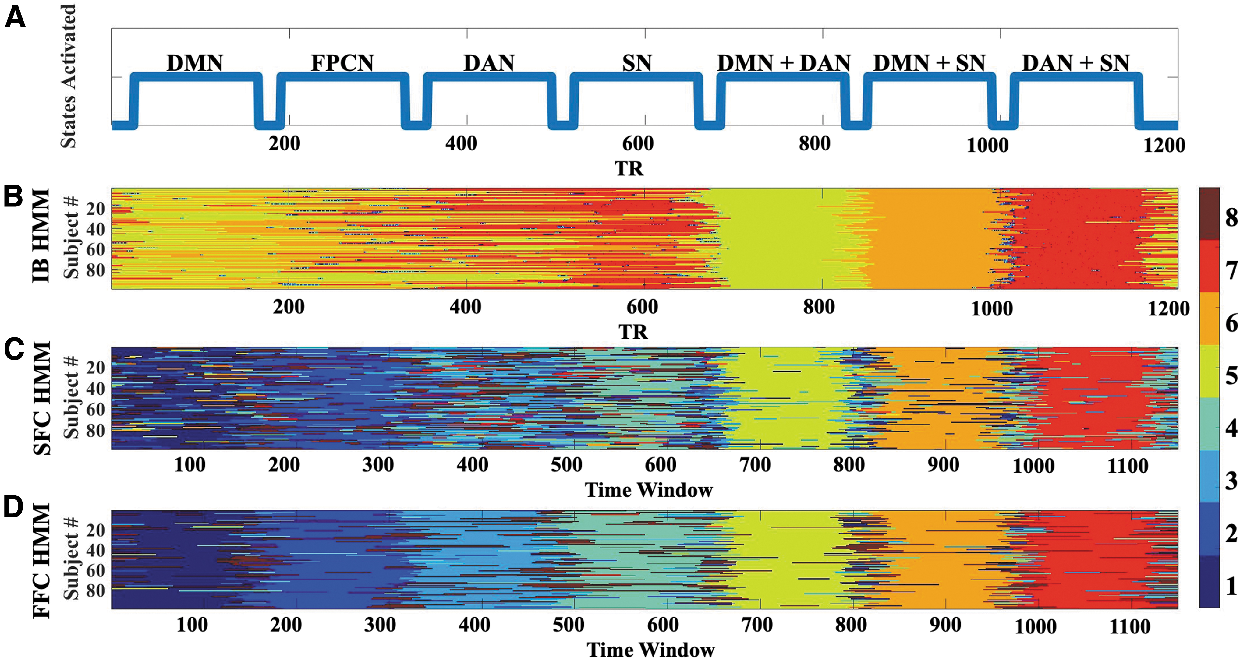
Verification of HMM connectivity-based states.
Unsurprisingly, IB HMM failed to adequately recover simulated pure connectivity states (Fig. 1B; mean R 2 between simulated and recovered Viterbi paths of 0.1741 ± 0.1569), although it appeared to recognize when two networks were “turned on” in conjunction. This may have occurred because there was more connectivity for the model to recognize: both within- and between-network connectivity. However, recall that IB HMM does not natively evaluate or recover connectivity states, so connectivity must be estimated through the process described in the Intensity-Based HMM section.
FFC HMM also showed strong performance in recovering the connectivity states themselves. A paired t-test on the Fisher-z transformed R 2 values between SFC and FFC HMMs indexing how similar each model's recovered connectivity states were to the induced states showed that FFC HMMs were significantly better at recovering induced states than SFC HMM [t(98) = 12.8745, p = 8.6087e-23]. (See Supplementary Appendix B for fuller discussion of the intensity-based states recovered by IB HMMs.)
Analysis of model outputs
We next evaluated the states themselves as well as their Viterbi paths. States from each model are distinguished with subscripts corresponding to the HMM from which they stem, that is, S1FFC corresponds to state 1 from FFC HMM. We present results from IB and SFC HMMs first to provide context for the differences in behavior exhibited by FFC HMM.
Connectivity state pattern analysis
First we examined IB HMM, which we did not expect to recover empirical connectivity states well. Unsurprisingly, the IB HMM differential functional connectivity states did not display strong distinguishing patterns either within or between the states (Fig. 2, top row). However, there were a few slight deviations from mean connectivity overall, especially in S4IB, S7IB, and S8IB. Nevertheless, these results show that a model not trained on connectivity states is, expectedly, not adept at recovering distinctive connectivity states.
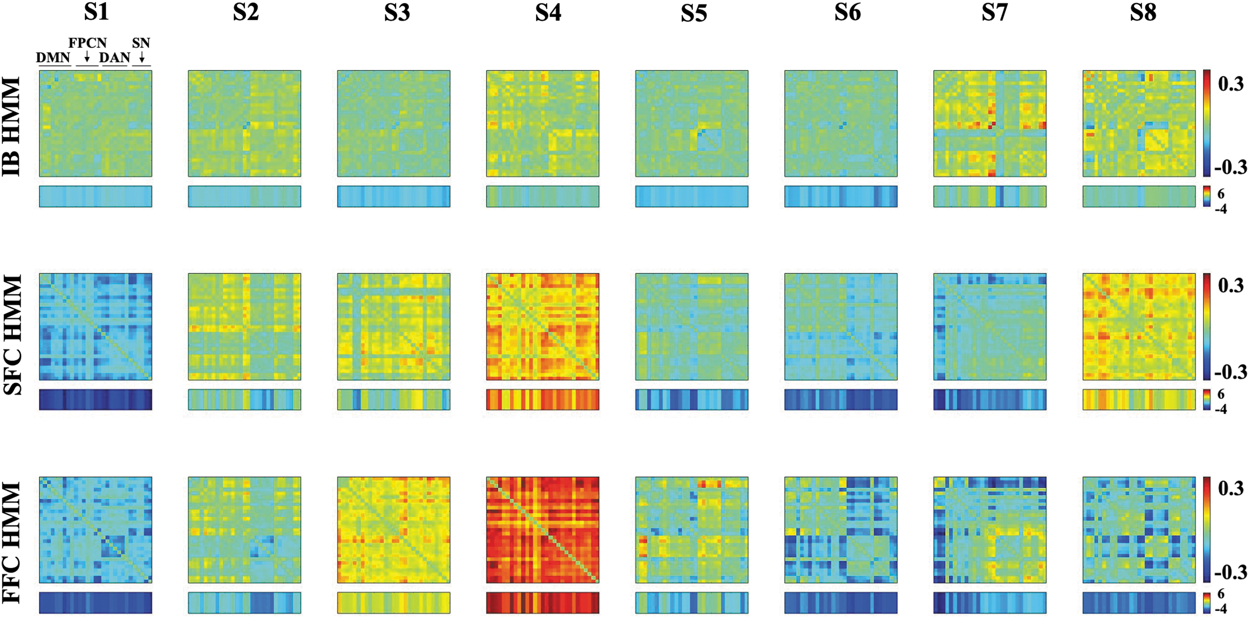
Differential functional connectivity states for SFC HMM (top row), FFC HMM (middle row), and IB HMM (bottom row). The summed connectivity vectors (summed across one dimension) are displayed below each state. The summed values for SFC were directly outputted from the model .while those for IB and FFC were calculated as described in Connectivity State Pattern Analysis section.
The critical benchmark for FFC HMM is therefore SFC HMM behavior. Can a model fitted to summed connectivity vectors nevertheless adequately recover full connectivity profiles? We observed that SFC HMM extracted distinct differential functional connectivity profiles across all eight states (Fig. 2, middle row). From visual examination, S1SFC showed below-baseline correlations among all networks, while elevated correlations compared to baseline were seen overall in S4SFC and S8SFC. Several states also showed distinct within-network changes in connectivity from baseline, with each state seeming to highlight a different network (e.g., S2SFC excludes within-network connectivity in DAN, while S3SFC and S5SFC exclude within-network connectivity in DMN).
Crucially, to what extent are FFC HMMs' connectivity states different from SFC HMM's? Visually, they appear to have poor correspondence (Fig. 2, bottom row). S4FFC showed strong above-average connectivity across all nodes—far stronger than that shown in S4SFC—and it was the only state to have overall above-average connectivity. In contrast, several other states showed a distinct reduction in functional connectivity specific to various networks. For example, S1FFC shows a within-network DAN disconnect, while S5FFC shows that DAN is connected to DMN and itself, but not the other networks. Moreover, S6FFC showed DAN and SN to be largely disconnected from DMN and FPCN, with DMN and FPCN connected to each other, while S7FFC showed strong disconnection between DMN and all other networks. Other patterns can also be found. Importantly, although, no SFC HMM state exhibited any of these patterns.
We next engaged in a quantitative comparison between states recovered by each model in two ways. First, we computed the pairwise Pearson correlations among all pairs of states (Fig. 3A). A one-to-one match in states would be illustrated with one large correlation coefficient (one orange/yellow square) and seven small correlations (seven green/blue squares) in each row. Yet this phenomenon was not observed, as it appears there are several states that might equally “match” across the two models from visual inspection.
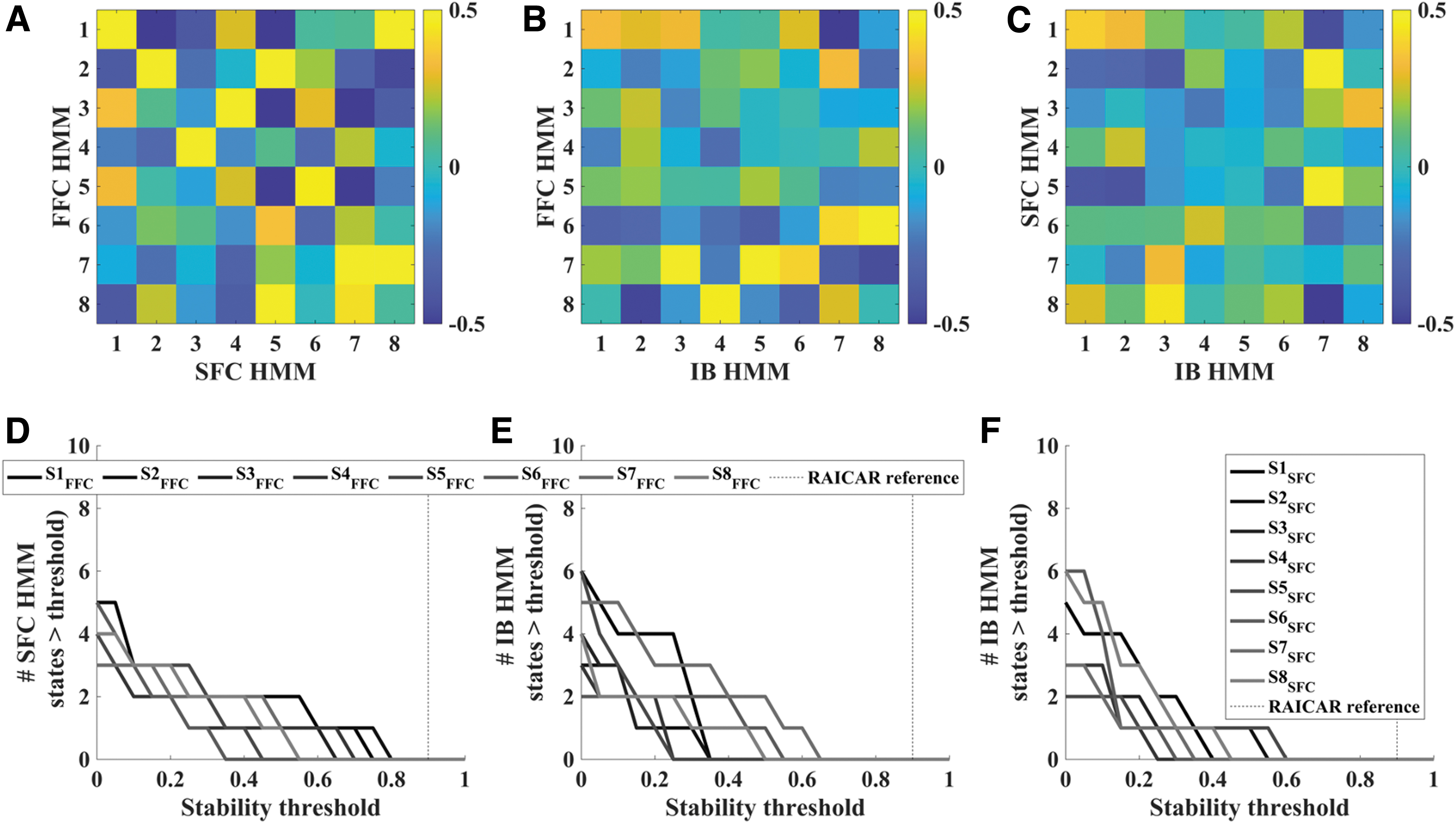
Pairwise comparisons between connectivity states discovered by each HMM show that each model recovered eight unique states. A one-to-one match between two states recovered by two different models would appear as a single orange/yellow square (high Pearson correlation) among seven green/blue squares (low Pearson correlation) in those two states' row or column combination. However,
Second, to quantitatively assess the degree to which there might be one-to-one state matching across states recovered by each pair of models, we took inspiration from the RAICAR analysis described above and sought to identify whether there was a threshold at which there would be a one-to-one state matching across all eight states found by both models. We are looking specifically for cases where a particular correlation threshold leads to exactly one SFC HMM state matching each of the FFC HMM states. We examined whether any possible correlation threshold in the range of 0–1 in steps of 0.05 would lead to exactly one SFC HMM, state matching each FFC HMM state by counting the number of SFC states that exceeded each possible threshold.
Visually, this accounts to counting how many “squares” in each row of Figure 3A surpass a particular value, with the goal being exactly one for all rows. This quantitative analysis confirmed the visual inspection results: There was no threshold for which all—or even most—FFC HMM states could achieve a unique mapping with exactly one SFC HMM state (Fig. 3D). This finding supports the interpretation that our novel FFC HMM recovers functional connectivity states that are distinct from those recovered by SFC HMM.
For completeness, we also repeated this analysis for comparisons between FFC HMM and IB HMM (Fig. 3B, E), as well as comparing SFC HMM and IB HMM (Fig. 3C, F). Results from these pairwise comparisons mirror those from the critical FFC versus SFC comparison: all three models appear to discover unique connectivity states, as there is no visual or quantitative correspondence between the states discovered by each model. Note that the comparisons with IB HMM are particularly informative, as they confirm that both FFC HMM and SFC HMM recovered states that reflected changes in connectivity patterns (in SFC HMM's case, summed connectivity vectors) and were robust to fluctuations in overall BOLD signal magnitude (i.e., the connectivity-based models did not end up simply discovering “connectivity” states based on fluctuations in average intensity). See Supplementary Appendix B for fuller discussion of intensity-based states recovered by IB HMM.
Finally, we also examined the relationship between SFC vectors from FFC HMM and SFC HMM. We found that the mean absolute value of the inner product of the summed connectivity vectors for matched states from each model was very high (0.84), suggesting that FFC HMMs' outputs can be used to reconstruct what SFC HMM would have recovered.
Viterbi path analysis
Viterbi paths can be visualized by assigning each state a color and plotting them for every person as a function of time point (repetition time [TR] in the fMRI time series, IB HMM, Fig. 4A) or time window (anchored on the first TR of the window, SFC HMM [Fig. 4B] and FFC HMM [Fig. 4C]) to show which states are active at each time point. These visualizations show that, compared to IB HMM, both connectivity-based HMMs appear “smoothed” over time, that is, transition among states more slowly; this is especially dramatic for FFC HMM. Autocorrelation and temporal discrepancy in input resolution between the intensity- versus connectivity-based HMMs—that is, IB HMM had a temporal resolution equal to that of the fMRI TR, while SFC and FFC HMMs had an effective sampling frequency on the order of 1 sample per 36 sec—likely contributing to this smoothing.
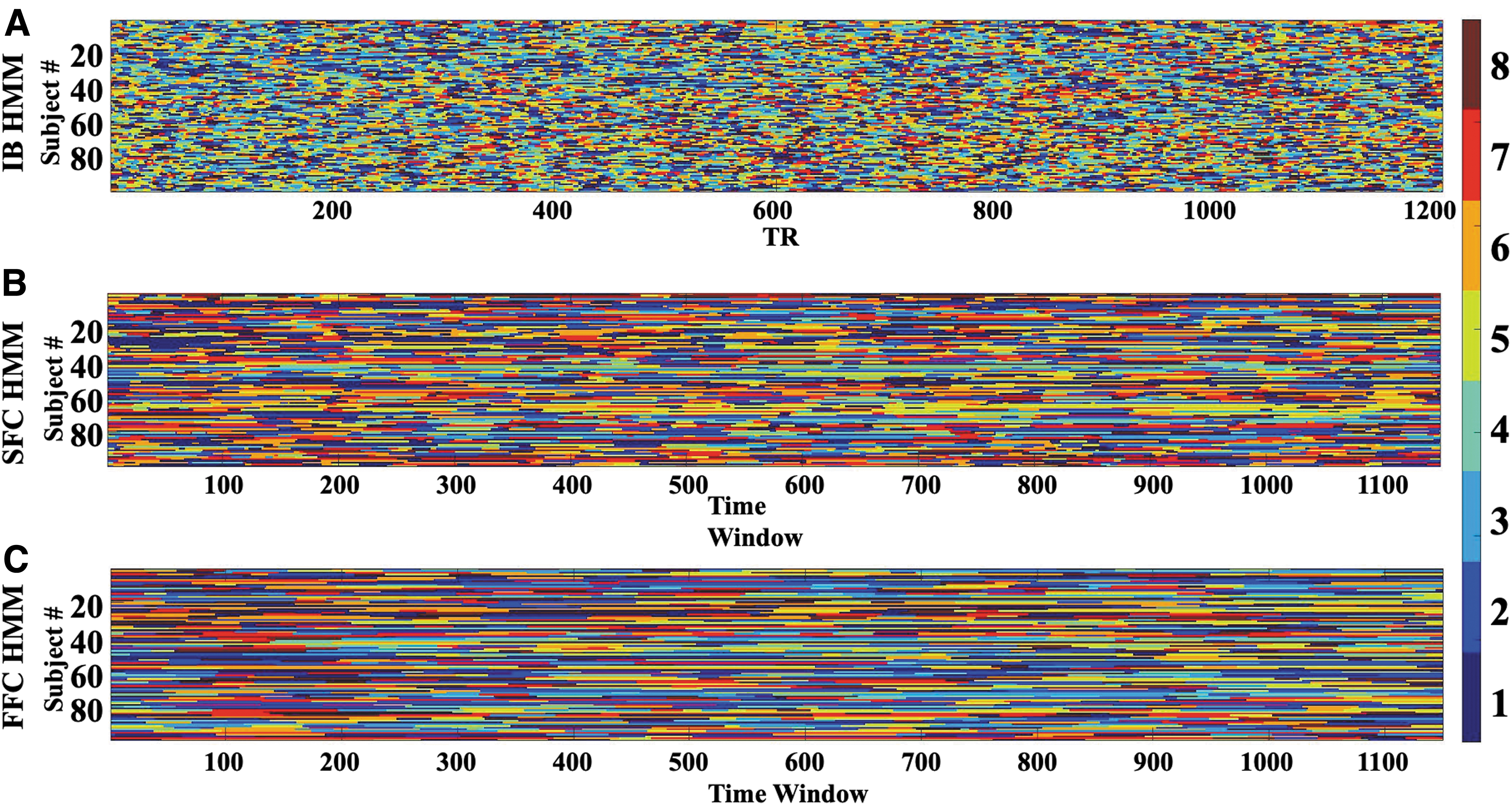
Viterbi Paths for
Interestingly, this temporal “smoothing” appears even more pronounced for FFC HMM than for SFC HMM—despite the fact that both SFC HMM and FFC HMM possess the same degree of “smoothing” in the input, that is, the same degree of autocorrelation induced by the sliding window computation of functional connectivity. We therefore suspect that FFC HMM complexity may have contributed to this behavior; we explore this possibility more in the Discussion section.
As a final check, we also confirmed that the Viterbi paths were robust to different realizations, that is, different initial conditions for model fitting. Recall that, although the RAICAR stability analyses determined eight states were ideal for all three models, state assignment (e.g., labeling a state as “S1” vs. “S8”) was initially arbitrary across all HMMs. Nevertheless, following state labeling alignment across initializations (Preliminary Model Fitting and Analysis section and Supplementary Appendices A.3 and C.1), we observed that the Viterbi path was reproducible across different realizations of the HMMs (R 2 ≥ ∼0.84) for all models tested: for all initializations, all models recognized the same connectivity states at the same time windows, and the same switches between states.
Discussion
In this study, we introduced an FFC HMM and investigated its ability to extract functional connectivity states in resting-state fMRI data. Using the HCP Unrelated 100, we fitted FFC HMM to a sliding window of functional connectivity from 29 ROIs across 4 networks (DMN, FPCN, DAN, and SN) and compared the connectivity states it discovered to those from two other models defined by SFC HMM (Ou et al, 2015) and intensity (IB HMM) (Eavani et al, 2013; Stevner et al, 2019; Vidaurre et al, 2017).
FFC HMMs' full connectivity states were starkly different from those recovered by SFC and IB HMMs, even as FFC HMM recovered simulated connectivity-based states more faithfully than either IB or SFC HMM. Thus, we should not assume that connectivity states derived from IB- or SFC-based HMMs reflect true connectivity states; FFC HMM is a more appropriate choice to examine and interpret pure functional connectivity profiles when the question of interest is based on connectivity and not intensity fluctuations.
Interestingly, our results revealed that FFC HMM changed states more slowly even with the same sliding window size as SFC HMM. The slower switching rate in FFC HMM may be due to the increased number of components fitted in FFC HMM (406 connectivity values per time window) compared to SFC HMM (29 components); this may reduce state switching by requiring broader changes in connectivity across multiple nodes to register a change in functional connectivity state. Interestingly, this behavior may indicate that FFC HMM is less sensitive to noise than SFC HMM.
Another possibility is that true functional connectivity may change quite slowly within a session, since it has been shown to be relatively stable across time with only moderate changes around the average (Vidaurre et al, 2021). Because SFC HMM sums across functional connectivities for a given node, such changes might accumulate and become comparably larger, causing SFC HMM to predict a state change when none is in fact present.
There are a number of key differences between our model and previous approaches that have targeted functional connectivity states using HMMs. In particular, Vidaurre (2021), Vidaurre et al (2021), and Vidaurre et al (2018a) fitted state-specific covariance matrices in a Gaussian HMM using intensity (BOLD or MEG based) as inputs. Notably, their approach assumed that the mean intensity level of the observed data did not change between states, that is, the mean activity was stationary across states (μ = 0 in the Gaussian model fitted by the HMM), thereby purposefully avoiding modeling changes in amplitude explicitly (Vidaurre, 2021). On the other hand, our approach uses covariance as the direct model input, sidestepping the assumption of stationarity in mean activity levels.
Other approaches have combined PCA and HMMs, either where PCA is done first and then the HMM fitted (Vidaurre et al, 2021), or where PCA and HMM fitting are done simultaneously (Vidaurre, 2021). In both cases, PCA is used to recover latent components in brain activity or connectivity data, which complicates the ability to interpret the discovered states with reference to known brain anatomy and functional networks. In the case of the second model (Vidaurre, 2021), this practice also suggests that the principal components discovered by the simultaneous approach can change as a function of connectivity state, such that the covariance matrix of one state may not refer to the same principal components as that of another state.
Finally, it has also been proposed that time delay-embedded HMMs may reveal functional connectivity networks in magnetoencephalography data (Vidaurre et al, 2018b). Although this approach has the advantage of being purely data driven and focused on phase-coupling network activity in the case of MEG data, it has not been applied to fMRI data and may encounter challenges due to its dependence on high temporal resolution and consequently long length of input data; we therefore leave exploration of this interesting possibility in fMRI data to future studies.
Limitations
HMMs assume independent Gaussians in the likelihood functions (Eddy, 2004; Eddy, 1996; Jurafsky and Martin, 2009; Rabiner, 1989; Rabiner and Juang, 1986), but one might note that using sliding window functional correlations as inputs (SFC and FFC HMMs) introduces autocorrelation. While we assumed independence as a simplifying assumption (Ou et al, 2015), we also conducted an exploratory analysis that varied window size to explore potential impact of autocorrelation magnitude. This analysis revealed that even large changes in sliding window length do not meaningfully impact the connectivity states recovered by either SFC HMM or FFC HMM (Supplementary Appendix C.4).
Therefore, we can feel confident that autocorrelation concerns do not unduly influence our findings. In fact, we note that independence may not strictly be assumed even for IB HMM or similar models, as the hemodynamic response function is continuous and therefore autocorrelation from one TR to the next is likely due to the poor temporal resolution of fMRI in general. The lack of dependence on sliding window length may also speak to whether sliding windows in general are an appropriate choice for HMM-based analysis of resting-state data, as this result may suggest that what the SFC and FFC HMMs may be recovering is a set of global, or relatively stable, functional connectivity states that the system slowly switches among as opposed to task-induced or more rapidly changing dynamic states.
Future research should investigate the relationship between global, unchanging dynamic connectivity profiles and the shifting profiles revealed by SFC HMM or FFC HMM, as well as in comparison to other methods proposed in the literature.
Gaussian HMMs also assume that the off-diagonal elements of the correlation matrices either are distributed normally or that violations of this assumption do not unduly affect results (Chen et al, 2016). In the absence of a model that explicitly estimates the covariance of such off-diagonal elements, we evaluated the impact of Fisher-z transforming the Pearson correlations before using them as inputs so that they would occupy a range of [−∞,∞] rather than [−1,1]. Transforming the Pearson correlations did not significantly affect the connectivity states recovered by FFC HMM (Supplementary Appendix C.4). We therefore elected to refrain from Fisher-z transforming to facilitate direct comparison to SFC HMM, which did not previously Fisher-z transform (Chen et al, 2016) and for which Fisher-z transformation is inappropriate because SFC HMM SFC vectors already occupy a range of [−∞,∞].
Finally, our results are also limited by the sliding window approach, as a given brain state may not persist for the entire sliding window, or signals from multiple brain states may overlap in the window. Other approaches may appear to remedy this shortcoming, such as spatial independent component analysis (Beckmann et al, 2005; Smith et al, 2012), structural equation modeling (Schlösser et al, 2003), or coactivation patterns in IB states (Liu and Duyn, 2013; Liu et al, 2013; Petridou et al, 2013). However, while these methods characterize spatial patterns of connectivity states, each time point is treated as independent and shuffling the time series does not affect spatial patterns of recovered brain states; they therefore only identify the states themselves and do not reveal the trajectory through state space. Thus, FFC HMM offers one of the best tools available to study the evolution of connectivity states over time.
Conclusions
We found that FFC HMM discovered connectivity states with more distinguishable patterns than those derived from HMMs with an intensity input (IB HMM) or summed connectivity input (SFC HMM), and which were fundamentally different from the functional connectivity profiles extracted by either of the other two methods. FFC HMM could also more faithfully recover simulated “ground truth” pure connectivity states. Because FFC HMM allows for a direct readout of connectivity-based states and their temporal evolution, it offers a powerful tool for extracting, analyzing, and understanding dynamic connectivities among brain regions.
Footnotes
Data/Code Availability Statement
Data from HCP are available from the HCP database (
Authors' Contributions
S.H.: conceptualization, formal analysis, investigation, methodology, project administration, software, validation, visualization, writing—original draft, and writing—review and editing. J.L.: investigation, methodology, supervision, validation, visualization, and writing—review and editing. A.R.S.: conceptualization, funding acquisition, investigation, methodology, project administration, supervision, validation, visualization, and writing—review and editing. X.P.H.: conceptualization, funding acquisition, investigation, methodology, project administration, resources, supervision, validation, visualization, and writing—review and editing. M.A.K.P.: conceptualization, funding acquisition, investigation, methodology, project administration, resources, supervision, validation, visualization, writing—original draft, and writing—review and editing.
Author Disclosure Statement
No competing financial interests exist.
Funding Information
This work was supported, in part, by the UCR NASA MIRO FIELDS Fellowship (to Sana Hussain). Data collection and sharing for this project were provided by the Human Connectome Project (HCP; Principal Investigators: Bruce Rosen, MD, PhD, Arthur W. Toga, PhD, Van J. Weeden, MD). HCP funding was provided by the National Institute of Dental and Craniofacial Research (NIDCR), the National Institute of Mental Health (NIMH), and the National Institute of Neurological Disorders and Stroke (NINDS). HCP data are disseminated by the Laboratory of Neuro Imaging at the University of Southern California. This work was funded by NIA R01 NS108638-01 (PIs: Xiaoping P. Hu and Aaron R. Seitz) and by the Canadian Institute for Advanced Research Azrieli Global Scholars Program (PI: Megan A.K. Peters). Funding sources had no involvement in the design and methodology of the study.
Supplementary Material
Supplementary Appendix A
Supplementary Appendix B
Supplementary Appendix C
References
Supplementary Material
Please find the following supplemental material available below.
For Open Access articles published under a Creative Commons License, all supplemental material carries the same license as the article it is associated with.
For non-Open Access articles published, all supplemental material carries a non-exclusive license, and permission requests for re-use of supplemental material or any part of supplemental material shall be sent directly to the copyright owner as specified in the copyright notice associated with the article.