Evidence of the Ability of Microsatellite Method to Distinguish Cannabis Strains with High Cannabinoid Content

Abstract

Introduction:

Cannabis is a plant with high potential for use in several sectors of the industry; however, it is also a controversial crop due to its tetrahydrocannabinol (THC) content. Moreover, the plant has a rather unclarified classification. Traditionally, two types of Cannabis have been distinguished, hemp as a source of fiber and low THC content, and marijuana with high THC levels, which is used as a drug. With the increasing use of CBD strains and wide range of commercially used THC strains, it is becoming paramount to be able to develop an easy and reliable method for Cannabis strain differentiation. The use of simple sequence repeat markers, or microsatellites, seems to be an applicable choice.

Materials and Methods:

In this study, 52 strains of Cannabis with variable cannabinoid content were collected from growers from different geographical regions and analyzed using 17 different microsatellite markers. For more precise differentiation, five strains were selected and a higher number of individuals of each were analyzed.

Results:

Fragment analysis and cluster analysis showed that when one to three individual plants per strain were analyzed, the method was able to classify these samples into distinguishable groups with similar gene structure. They also revealed that when a larger sample set was used (10 individual plants per strain), highly specific strain clusters could be fully discriminated.

Conclusion:

Our study involved the highest number of cannabinoid-rich strains up to now and showed that the microsatellite method can be used to reliably differentiate Cannabis strains and show their relationships.

Introduction

Cannabis has been cultivated worldwide and is used as a source of fiber, medicinal substances, and drugs.¹ It is a member of the Cannabaceae family, is diploid, and has nine pairs of autosomes and a pair of gonosomes. It is usually a dioecious plant.² Cannabis can be divided into two main groups: hemp, with low tetrahydrocannabinol (THC) content, used mainly for fiber, and marijuana, with higher THC content, which is often used for drugs.³

Taxonomy of Cannabis has undergone many changes. Historically, the genus Cannabis was divided into two species, Cannabis sativa and Cannabis indica; this was, however, later rejected.^4,5 With the description of Cannabis ruderalis, an attempt for the reestablishment of these two species appeared and C. sativa and C. indica were also recognized as subspecies of C. sativa.^6,7 Recently, Cannabis is mostly seen as a single highly variable species, despite genetic studies suggesting them as distinct species.^8,9 Many varieties of Cannabis have also been named without being registered as cultivars and should be named as Cannabis strains.¹⁰

Numerous variants of Cannabis and its use in multiple fields make methods for its exact differentiation essential. It is important to develop means to analyze Cannabis DNA to identify strains and track sample origin. In the forensic field, marijuana needs to be differentiated from low-THC Cannabis, whereas in hemp used for fiber, identification of variability among its genotypes is essential for the improvement of crops. Many strains of Cannabis are often misidentified and their genome is influenced by their geographic origin. In addition, Cannabis genomic identification is complicated by the fact that the plants are often cultivated by clonal propagation and may show aneuploidy, polyploidy, or multiple gene loci.¹¹ Development of methods to differentiate Cannabis has increased lately, and one type of them uses the analysis of simple sequence repeats (SSRs).^12–16

SSRs, also known as microsatellites, or short tandem repeats, have distinct advantages compared to other methods.^17,18 They are codominant, give reproducible results, have high discriminatory power, and can be multiplexed.¹⁹ Microsatellite analysis in Cannabis helps understand its genome, which could lead to the successful cultivation of plants with accurate cannabinoid profiles and also to bring about progress in Cannabis breeding. However, only small-scale SSR markers have been reported in Cannabis.^1,3,20 Gilmore and Peakall developed the first 15 variable microsatellite loci in 48 samples of C. sativa, which allow discrimination among individuals and accessions and thus help characterize genetic diversity in cultivated and natural Cannabis populations.¹ Another 11 markers were developed by Alghanim and Almirall.³ Microsatellites have since been used to identify hemp cultivars or to distinguish forensic marijuana samples.^14,21–26

However, few studies have aimed to differentiate between individual strains of Cannabis with high cannabinoid content. In this study, we aimed to differentiate samples belonging to a larger group of strains by using a combination of markers previously used in various studies. Fifty-two different strains of Cannabis, mostly with high cannabinoid content, were analyzed using 17 selected markers to determine whether they could be grouped into similar or identical genetic clusters by the microsatellite method. We also evaluated whether there was any relationship between the clusters and the geographical origin of the strains.

Materials and Methods

Ethics statement

This research did not contain any study involving animal or human participants, nor did it take place in any private or protected area. No specific permission was required for corresponding locations.

Cannabis samples and growth conditions

Samples belonging to 52 Cannabis strains with high CBD and THC contents, as well as one hemp variety, were collected from growers from different geographical regions (Table 1). Each strain was represented by one to three plants with the total of 88 individuals. Five selected strains (Ultimate, Orange Hill Special, Snow Bud, CBD Skunk Haze, and Durban Poison) were used in the cultivation experiment and grown under the same conditions, providing 10 individual plants of each strain to test whether there was an increase in strain identification accuracy.

Table 1.

Analyzed Cannabis Strains, Their Source, Cannabinoid Content, and Type

Strain	Abbreviation	Source	CBD content^a	THC content^a	Type^b
No. 49 CBD	C49	Sensi Seeds	High	Low	Hybrid
Black domina CBD No. 743	CBL	Sensi Seeds	Medium	High	Hybrid
Blueberry	BBR	Dutch Passion	Low	Very high	indica
Blue Gelato	BLG	Barneys Farm	Low	High	Hybrid
Bubblegum XL	BXL	RQS	Low	Very high	Hybrid
California Gold	CAG	Paradise Seeds	Low	Very high	indica
CBD E3D	E3D7	CBD Crew	Medium	Low	sativa
CBD Skunk Haze	CSH	Dutch Passion	Medium	Medium	Hybrid
CBD Sweet and sour Widow	ECC	CBD Crew	High	Medium	sativa
CBD Therapy	THE	CBD Crew	Medium	Low	Hybrid
CBD US	EUS	USA^c	High	Low	Hybrid
Charllotes Angel	CAN	Dutch Passion	Very high	Low	sativa
Critical	CCL	Barneys Farm	Low	High	indica
Critical Mass	CCM	Dinafem	Low	Very high	indica
Durban Poison	DP	Dutch Passion	Low	High	sativa
Durga Mata II CBD	DUM	Paradise Seeds	High	Medium	indica
Dutch Kush	DUK	Paradise Seeds	Low	Very high	indica
Euforia	EEA	Dutch Passion	Low	Very high	sativa
Fat Banana	FAB	RQS	Low	Very high	indica
Gelato Olandese	GOL	DutchFem	Low	Very high	sativa
Glookies	GLO	Barneys Farm	Low	Very high	indica
Glueberry OG	GBO	Dutch Passion	Low	Very high	Hybrid
Green Gelato	GGO	RQS	Low	Very high	Hybrid
HiFi 4g	HIF	Dutch Passion	Low	Very high	Hybrid
Hulkberry	HUL	RQS	Low	Very high	Hybrid
Ice Cream	ICC	Paradise Seeds	Low	Very high	Hybrid
Kompolti	KOM	Hempoint	Medium	Low	sativa
Lost Coast OG	LCO	Humboldt	Low	Very high	indica
LSD	LSD	Barneys Farm	Low	Very high	indica
Masterkush	MAK	Dutch Passion	Low	High	indica
Mendocino Skunk	MES	Paradise Seeds	Low	Very high	Hybrid
Moby Dick CBD	MOD	Dinafem	High	Medium	Hybrid
Mokums Tulip	MKT	Dutch Passion	Low	Very high	Hybrid
Momo	MOM	Czech Republic^c	High	Low	Hybrid
Nebula	NEB	Paradise Seeds	Low	Very high	Hybrid
Orange Hill Special	OHS	Dutch Passion	Low	Very high	Hybrid
Original cheese	ORC	Paradise Seeds	Low	Very high	Hybrid
Painkiller XL	PXL	RQS	High	Medium	sativa
Peyote Cookies Critical	PCC	Barneys Farm	Low	High	indica
Power Plant	PPT	Dutch Passion	Low	High	Hybrid
Remo Chemo	RCH	Dinafem	Low	Very high	Hybrid
Royal Gorilla	ROG	RQS	Low	Very high	Hybrid
Royal Highness	RHS	RQS	High	High	Hybrid
Sensi Star	SST	Paradise Seeds	Low	Very high	indica
Snow Bud	SB	Dutch Passion	Low	Medium	Hybrid
Strawberry Cough	STC	Dutch Passion	Low	High	sativa
Strawberry Lemonade	STL	Barneys Farm	Low	Very high	Hybrid
Sweet Zkittles	SZS	RQS	Low	Very high	indica
Ultimate	ULT	Dutch Passion	Low	Very high	Hybrid
Vanilla Kush	VAK	Barneys Farm	Medium	Very high	indica
Wappa	WAP	Paradise Seeds	Low	Very high	Hybrid
White Siberian	WSI	Dinafem	Low	Very high	indica

Cannabinoid content was categorized as follows: low, under 5%; medium, 5–10%; high, 10–15%; and very high, over 15%.

For the uncertain taxonomy of Cannabis, the collected strains were categorized into geographical types, sometimes referred to as species or subspecies, Cannabis sativa and Cannabis indica; when neither type was predominant with at least 70%, the strain was categorized as hybrid.

Momo and CBD US were taken from experiments in Czech Republic and United States (respectively).

CBD, cannabidiol; THC, tetrahydrocannabinol.

All plants were grown from seeds in Cannabis research facilities at Rabbit, Trhový Štěpánov, Czech Republic. Before planting in the growing system, the seeds were left in water for 24 h at 21°C and placed into rockwool seeding rollers for germination. After growing out of the rollers, the plants were moved into AutoPot pots with a volume of 15 L filled with lightly organically fertilized substrate Light-Mix (BioBizz). The organic additives Startrex and Mycotrex (BioTabs), containing PGPR and saprophytic fungi, were added to the substrate. When the seedlings were planted, the main organic fertilizer, with gradual release in the form of tablets, was added. The pots were then filled with a mixture of Orgatrex and Bactrex (BioTabs) dissolved in water, as recommended. Plants were watered automatically, and fertilizers were supplied in quantities and on dates recommended by the fertilizer manufacturer.

SanLight LED modules were used with a total power of 3,150 W to illuminate the plants. Throughout the growth cycle, the plants were exposed to a light regime of 20-h light/4-h dark. The average air temperature reached the level of 26.4°C, the average relative humidity of the air 66.6%, and the CO₂ content an average value of 856 ppm.

Isolation of Cannabis DNA

Two leaves were collected from each individual, and all samples were dried on silica gel. For DNA isolation, 20 mg of the prepared plant tissue from each sample was homogenized using TissueLyser II (Qiagen, Hilden, Germany). DNA was isolated from all samples using DNeasy Plant Mini Kit (Qiagen) according to the manufacturer's instructions and dissolved in distilled water.²⁷ DNA quality and concentration were evaluated using NanoDrop 2000 Spectrophotometer (Thermo Fisher Scientific, Waltham, MA, USA). DNA was diluted to the concentration of 20 ng/μL and subsequently used as a template for PCR reaction.

Selection of microsatellite markers

Primers for amplification of microsatellite markers were selected from previous studies. Only markers with three or more base repetitions were selected because of their high variability among plant varieties. From 22 markers, we further selected 17 markers showing variability among the analyzed plant samples (Table 2).

Table 2.

Primers Selected for the Amplification of Microsatellite Markers (Only Markers Used in Final Reactions Shown)

Marker	Forward sequence^a	Reverse sequence	Final primer concentration in reaction [nM]	Product size^b	Repeat motif
ANUCS 301¹	PET: ATA TGG TTG AAA TCC ATT GC	TAA CAA AGT TTC GTG AGG GT	4^c	130–258	(TTA)₁₅
ANUCS 302¹	NED: AAC ATA AAC ACC AAC AAC TGC	ATG GTT GAT GTT TTG ATG GT	0.15^d	130–167	(CAA)₇-(CAA)₄
ANUCS 304¹	FAM: TCT TCA CTC ACC TCC TCT CT	TCT TTA AGC GGG ACT CGT	2^d	140–206	(CAA)₇TCA(TCT)₇
B01-CANN1¹¹	FAM: TGG AGT CAA ATG AAA GGG AAC	CCA TAG CAT TAT CCC ACT CAA G	1.5^e	314–370	(GAA)₁₃(A)(GAA)₃
B02-CANN2¹¹	VIC: CAA CCA AAT GAG AAT GCA ACC	TGT TTT CTT CAC TGC ACC C	0.15^d	167–175	(AAG)₁₀
B05-CANN1¹¹	VIC: TTG ATG GTG GTG AAA CGG C	CCC CAA TCT CAA TCT CAA CCC	0.15^f	243–249	(TTG)₉
C11-CANN1¹¹	FAM: GTG GTG GTG ATG ATG ATA ATG G	TGA ATT GGT TAC GAT GGC G	0.15^f	152–178	(GAT)₈(GGT)₇
D02-CANN1¹¹	VIC: GGT TGG GAT GTT GTT GTT GTG	AGA AAT CCA AGG TCC TGA TGG	0.15^f	106–118	(GTT)₇
E07-CANN1¹¹	PET: CAA ATG CCA CAC CAC CTT C	GTG GTA GCC AGG TAT AGG TAG	0.15^d	104–116	(CTA)₉
H06-CANN2¹¹	NED: TGG TTT CAG TGG TCC TCT C	ACG TGA GTG ATG ACA CGA G	0.15^d	269–275	(ACG)₇
CAN0010¹⁴	PET: TCC AAA CGT TCT CTC TCT CC	CTA CTA ACC CAA TCA GAC CCA	0.15^e	270–282	(GTG)₆
CAN0051¹⁴	VIC: AAC CCA AAA GAG CTG AGA GA	CTC AGC AAG GTG AGT ACA CG	0.15^g	291–320	(TCA)₆
CAN0126¹⁴	PET: GAG TAA GAG AAG GCG AAC CA	CCT GTG TAA CAG AAA ACC CC	0.15^g	181–192	(AATACC)₃(CAG)₆
CAN0585¹⁴	VIC: TCA TCA TCA TCC CTC CCT AT	GGT CCA TAG TTG GCT GAT CT	0.15^g	205–235	(ACTTCTATT)₂T(CAAAAC)₃
CAN1347¹⁴	PET: TGT TTC TAA GGC TCA GTC CC	GGC AAA GGT AAA GCA AGT GT	0.25^e	216–227	(AAC)₆(ATC)₇
CAN1419¹⁴	NED: TGA GGA TCA TCA TGG TTC AG	TTT TCC TTC TCC GCT ACA TC	2^e	247–276	(CAGAAC)₃CAA(AACCAG)₃
CAN2913¹⁴	FAM: AGG AAC ACT TTG AAA GCG AG	CGG TCA TCT ACC TTG AGC TT	0.15^e	120–140	(AAG)₇

Used fluorescent dye on forward primers after multiplex optimization is included in the sequence: FAM, blue; PET, red; VIC, green; NED, yellow.

Product size of alleles detected in this study.

Multiplex 4b.

Multiplex 3.

Multiplex 2.

Multiplex 4a.

Multiplex 1.

Optimization of the PCR multiplexes

Primers for the 17 selected microsatellite markers were divided into four multiplexes according to Multiplex Manager v 1.2.²⁸ After optimization, which included changes in primer combination in multiplexes, annealing temperature, and time of elongation, one of the primers from Multiplex 4 was excluded and used separately in a singleplex reaction. The multiplexes are listed in Table 2.

PCR reaction

The PCR protocol was performed according to Gilmore and Peakall, with changes due to optimization.¹ Multiplexes consisted of 2.5 μL Multiplex PCR Master Mix (Qiagen) per sample, primers as shown in Table 2, 0.5 μL template DNA, and H₂O to 5 μL total reaction volume per sample. The reaction comprised a pre-denaturation at 94°C for 15 min, then 35 cycles of 94°C for 30 sec, 53°C or 57°C for 40 sec, and 72°C for 30 sec, and a final elongation step at 72°C for 10 min.

Annealing temperature in multiplex 1 and 2 was 57°C, whereas in multiplex 3 and 4a and singleplex 4b, it was 53°C. The PCR products were subsequently diluted as follows: multiplex 1 product was diluted 10 times, and multiplex 2, 4a, and singleplex 4b products were diluted 5 times. PCR products were separated by agarose gel electrophoresis with 2% agarose to confirm the presence and size range of amplified markers. As a ladder, GeneRuler 100 bp DNA Ladder (Thermo Fisher Scientific) was used, and as loading dye, we used 6×DNA Loading Dye (Thermo Fisher Scientific).

Fragment analysis

Each PCR product (1 μL) was mixed with 12.1 μL of a 120:1 solution of formamide:size standard (GeneScan 500 LIZ; Thermo Fisher Scientific). Multiplex 4a and singleplex 4b were both added to the same mixture. The prepared samples were then centrifuged using Centrifuge 5430 (Eppendorf, Hamburg, Germany) and denatured on Veriti Thermal Cycler (Thermo Fisher Scientific). Denatured PCR products were then prepared for fragment analysis.

Fragment lengths were determined by fragment analysis on ABI 3130 Genetic Analyzer and evaluated using GeneMapper 4.0 (Thermo Fisher Scientific), which visualized alleles as color-coded peaks. Genotyping was performed in 17 markers that showed variability between strains. The lengths of amplicons were rounded to the nearest base pair. In case two different amplicons with the difference of 1 bp were detected, the later detected amplicon was changed to the one detected previously.

Clustering of individual plants

The relatedness of individuals and their division into clusters was performed using Structure software, version 2.3.4, which divided individual plants into clusters according to the likelihood and similarity of results during multiple runs.²⁹ Each population was characterized by the frequency of alleles in each locus, and the individuals were assigned to one or more populations. The length of the burnin period, representing the number of Markov chain Monte Carlo steps until the results are in balance, was initially set to 10,000, and the number of steps after the burnin period to 50,000 to infer the number of clusters (K). Subsequently, the length of the burnin period was increased to 500,000 and the number of steps after the burnin period to 750,000. The number of iterations for each K was set to 20.

For the determination of optimal K and data visualization, we used MS Excel and Structure Harvester online tool.³⁰ The distances between individuals were then visualized by principal coordinate analysis (PCA) with Lynch distance using the POLYSAT package in R version 4.2.0.

SPAGeDi1-5d was used to determine the number of alleles, allelic richness, gene diversity, observed heterozygosity, and inbreeding coefficient.³¹

Results

Microsatellite markers used in previous studies were adjusted for the analysis of high-cannabinoid strains included in this project. After optimization, 17 markers were selected to determine the genetic diversity of 52 Cannabis strains. Agarose gel electrophoresis revealed the size range of amplified markers (Supplementary Fig. S1). Size of all amplified markers for each strain is listed in Supplementary Tables S1 and S2.

Samples were analyzed using Structure software for every possible number of populations (K=1–88), and the highest value of K was identified by Structure Harvester as the value for which the individual samples were best divided into clusters (Supplementary Fig. S2). This value was identified as K=4 and was set for the subsequent analysis with a greater length of burnin period and number of steps after the burnin period for more accurate results.

The clustering divided alleles into four large groups, and the individual samples belonging to 52 strains were mostly classified into all four to a greater or lesser extent, with one group being predominant (Fig. 1 and Supplementary Table S3). Similar profiles were observed for multiple individuals within the four groups. This was the case for all the individuals belonging to the same strain. Some strains had a distinct profile different from other strains, but similarities in individuals of different strains were also detected, which implied the relatedness of some Cannabis strains.

FIG. 1.

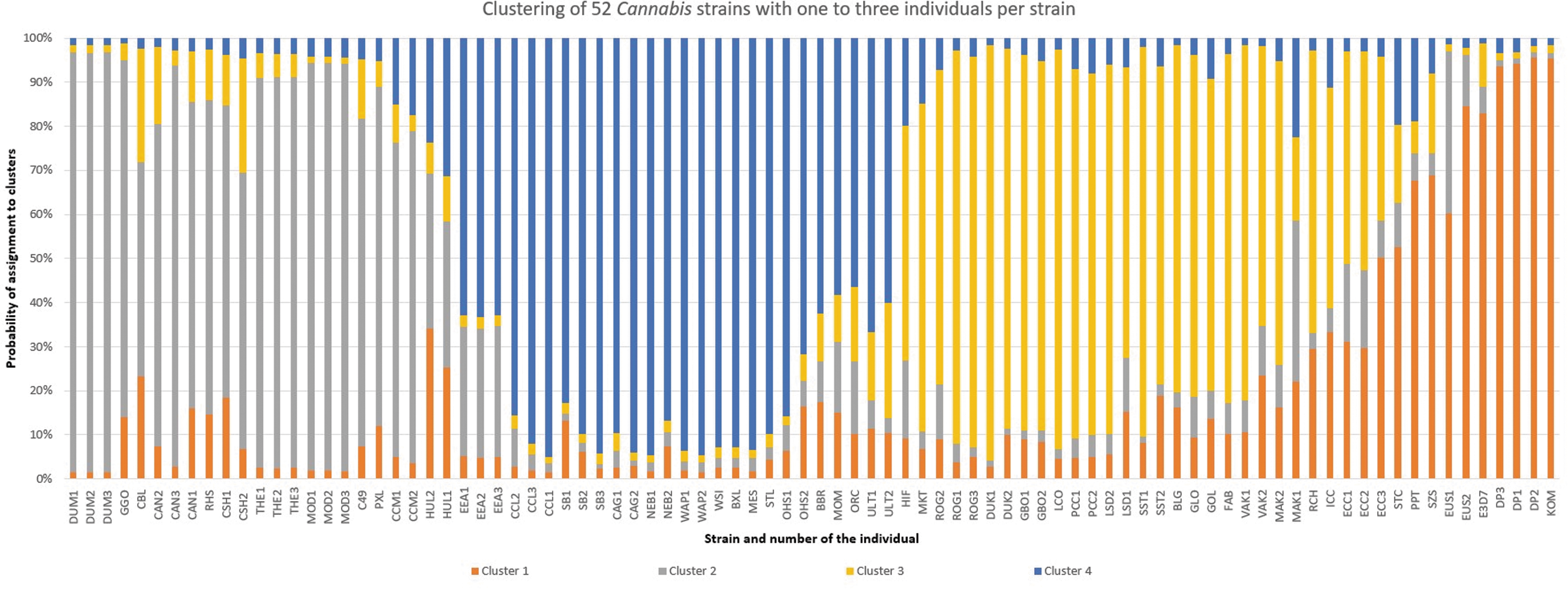
Clustering of 52 Cannabis strains with one to three individuals per strain using MS Excel. See Table 1 for strain abbreviations.

A larger number of individuals per strain were analyzed to further divide individuals into strain-specific groups. Five strains were selected for this experiment, each represented by 10 individuals. Samples were analyzed using the same method, and the individuals formed five distinct clusters, each corresponding to their strain (Fig. 2 and Supplementary Fig. S3). Only minor similarities were detected between the strains.

FIG. 2.

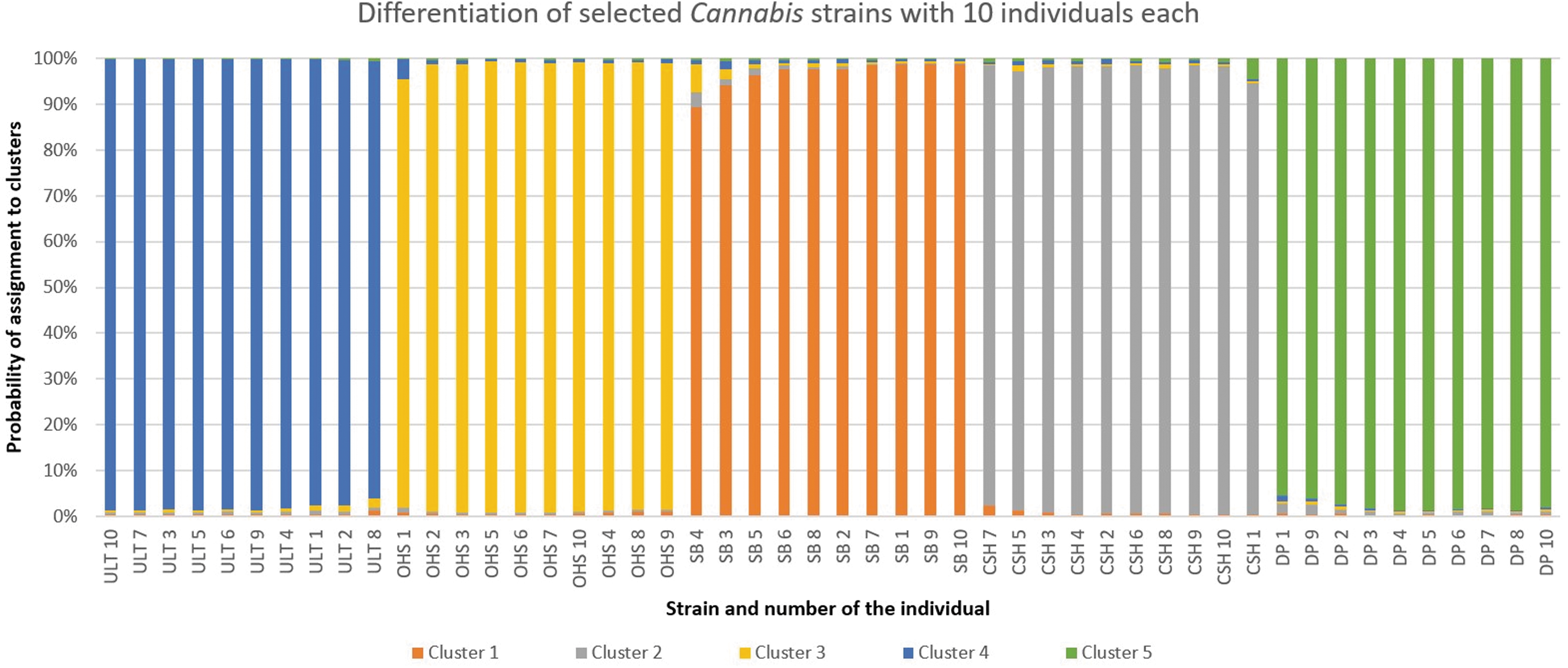
Differentiation of five Cannabis strains with a higher number of individuals per strain using MS Excel. See Table 1 for strain abbreviations.

The distances between five Cannabis strains with 10 individuals each were also visualized using R version 4.2.0, with the POLYSAT package. PCA with Lynch distance was chosen for the visualization for it proved better in distinguishing populations (Fig. 3).

FIG. 3.

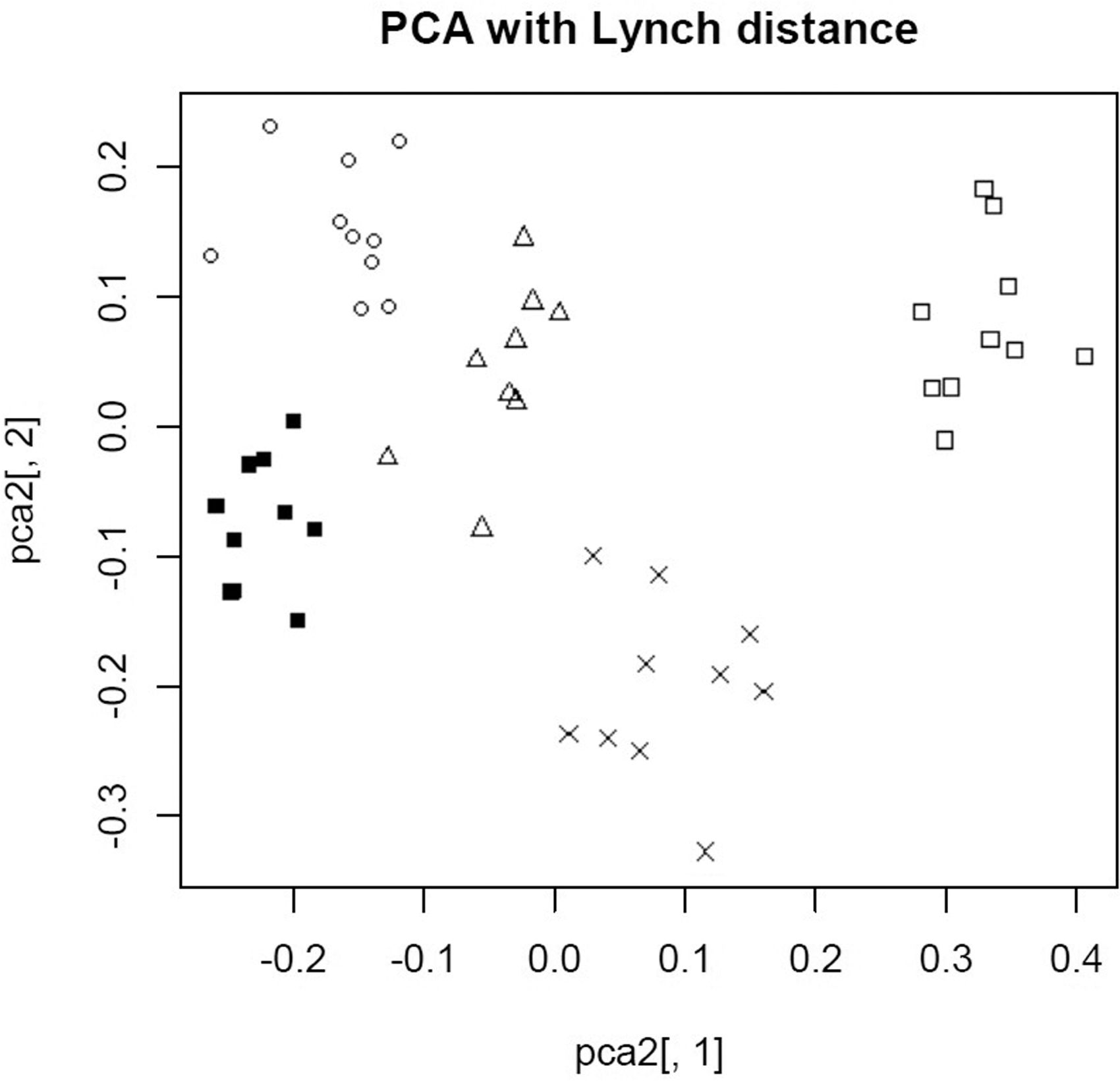
Visualization of genetic distances between individuals by PCA with Lynch distance. Individuals belonging to each strain indicated by symbols: circle, Orange Hill Special; triangle, Snow Bud; square, Durban Poison; fill square, Ultimate; cross, CBD Skunk Haze. PCA, principal coordinate analysis.

The number of alleles and the expected and observed heterozygosity (Table 3) were calculated using SPAGeDi1-5d. The number of alleles ranged from two to eight, the expected heterozygosity ranged from 0.00 to 0.74, and the observed heterozygosity ranged from 0.00 to 1.00. Observed heterozygosity was usually significantly higher than expected. A significant deviation from Hardy–Weinberg equilibrium was found in all populations.

Table 3.

Number of Alleles, Expected and Observed Heterozygosity Determined by SPAGeDi1-5d

	ULT			OHS			SB			CSH			DP
Locus	NA	He	Ho	NA	He	Ho	NA	He	Ho	NA	He	Ho	NA	He	Ho
CAN0126	1	0.00	0.00	2	0.47	0.50	1	0.00	0.00	2	0.52	0.20	3	0.54	0.60
CAN0585	3	0.56	1.00	3	0.69	1.00	3	0.67	1.00	2	0.53	1.00	3	0.59	1.00
CAN0051	2	0.51	0.30	1	0.00	0.00	2	0.50	0.40	1	0.00	0.00	3	0.53	0.70
CAN2913	2	0.53	1.00	4	0.76	1.00	4	0.67	1.00	1	0.00	0.00	3	0.70	1.00
CAN1347	1	0.00	0.00	1	0.00	0.00	1	0.00	0.00	2	0.50	0.60	3	0.62	0.60
CAN0010	2	0.52	0.50	2	0.50	0.60	2	0.53	1.00	1	0.00	0.00	2	0.39	0.50
B01-CANN1	1	0.00	0.00	1	0.00	0.00	1	0.00	0.00	1	0.00	0.00	2	0.44	0.60
CAN1419	2	0.50	0.40	1	0.00	0.00	2	0.39	0.30	2	0.51	0.30	3	0.28	0.30
E07-CANN1	2	0.53	1.00	2	0.53	1.00	3	0.51	0.70	2	0.44	0.60	2	0.44	0.40
ANUCS302	2	0.39	0.30	4	0.72	0.90	3	0.56	0.60	4	0.70	0.80	3	0.28	0.30
B02-CANN2	2	0.52	0.50	2	0.52	0.70	1	0.00	0.00	2	0.19	0.20	1	0.00	0.00
ANUCS304	1	0.00	0.00	1	0.00	0.00	1	0.00	0.00	4	0.68	0.30	4	0.60	0.20
H06-CANN2	2	0.39	0.50	2	0.52	0.40	3	0.64	0.70	2	0.48	0.70	3	0.70	1.00
D02-CANN1	1	0.00	0.00	2	0.52	0.40	2	0.52	0.70	2	0.53	1.00	2	0.53	1.00
C11-CANN1	2	0.52	0.50	1	0.00	0.00	2	0.39	0.50	3	0.54	0.70	3	0.69	1.00
B05-CANN1	2	0.52	0.40	1	0.00	0.00	2	0.19	0.20	1	0.00	0.00	3	0.59	1.00
ANUCS301	3	0.66	0.90	3	0.62	0.80	3	0.67	1.00	6	0.76	1.00	1	0.00	0.00

Number of alleles (NA), expected heterozygosity (He), and observed heterozygosity (Ho) in tested strains with 10 individuals each and all tested markers.

CSH, CBD Skunk Haze; DP, Durban Poison; OHS, Orange Hill Special; SB, Snow Bud; ULT, Ultimate.

Discussion

For the increasing use of Cannabis plants containing cannabinoids for medical purposes, it is necessary to develop effective methods able to identify Cannabis strains with known cannabinoid content and analyze their relatedness. Our work aimed to distinguish 52 mostly high-cannabinoid strains with 17 microsatellite markers and correctly classified individual samples into four clusters of similar strains. When testing a higher number of individuals per strain, all tested strains were clearly distinguished. Previous studies used microsatellite analysis mostly to individualize samples of hemp and marijuana, differentiate hemp cultivars, and identify the origin of Cannabis samples.^{11,14,21–26,32–35} Only few studies have aimed to differentiate between individual strains with high cannabinoid content.^24,36,37

Schwabe and McGlaughlin developed 10 new microsatellite markers to analyze differences in 122 samples belonging to 30 commercially available C. sativa strains, whereas Soler et al used 6 SSR markers for genotyping 154 individual plants of 20 cultivars, and Dufresnes et al analyzed 24 hemp varieties and 15 marijuana varieties with 13 microsatellite markers.^24,36,37 Our work analyzed a higher number of strains using 17 markers. These studies have found similarities in different strains and variability within the same strain, which are likely caused by mislabeling and misidentification, which we did not observe in our study. Dufresnes et al also detected lower diversity within marijuana varieties, and substantially higher genetic distances among them compared to hemp, which is consistent with our results.²⁴

Although some strains of geographical types sativa, indica, and hybrid clustered together, we did not find any genetic distinction between them, similar to previous studies.³⁶

Most markers used had a product size in or close to the range documented in previous studies.^1,11,14 The exception was marker CAN1347, where the previously documented product had a size of 133 bp, whereas in our strains, the size range was 216–227 bp.

We detected 2 to 13 alleles per locus in all tested samples, with the average of 6.06, and heterozygosity ranging from 0.0 to 1.0 (average=0.47). Heterozygosity was determined for five strains with 10 individuals, as some of the 52 strains did not have enough individuals. Our results were similar to those previously observed, with high polymorphism and heterozygosity. Gilmore and Peakall detected an average of 10 alleles per locus, with the range of 2–28, and mean heterozygosity of 0.68, ranging from 0.28 to 0.94.¹ Soler et al observed very high polymorphism with an average of 17 alleles, with heterozygosity average values of 0.753 and 0.429 for C. sativa var. indica and C. sativa var. sativa, respectively.³⁷ Borin et al observed comparable heterozygosity among all varieties, which was on average 0.58±0.09, while Dufresnes et al detected heterozygosity of 0.41±0.15.^24,33

Observed heterozygosity was usually significantly higher than expected and often reached a value of 1.0. A significant deviation from the Hardy–Weinberg equilibrium was found in all populations. This was likely caused by the high number of alleles for each marker, which led to high genetic variability. The populations were not natural, and some of the strains were polyploid.

In Cannabis, in addition to seed propagation, cloning is also used, which leads to new genetically identical plants.^24,38 High clonality leads to greater allele and genotype representation of the largest clones relative to the smaller ones.³⁹ That explains the deviation from Hardy-Weinberg equilibrium as well as small differences between individuals of the same strain.

Conclusions

Fifty-two Cannabis strains with mostly high cannabinoid content were analyzed using microsatellite markers. While a low number of plants (one to three) were used for analysis, the method was able to divide strains into four distinct clusters with groups of individuals showing more similar profiles, which mostly belonged to the same strain, as well as apparent relationships between strains. When a higher number of individuals per strain (10 plants) were used for the analysis, all individuals were correctly assigned to their particular strain. In this research, for the first time, the method was applied to such a large number of Cannabis strains with high cannabinoid content, and individuals of different strains were clearly distinguished. Our results will help differentiate Cannabis strains of unknown or unsure origin, determine their relatedness to other strains, and unambiguously identify the strain of an unknown sample.

Footnotes

Acknowledgments

We thank Zdeněk Jandejsek and Rabbit, a. s., Trhový Štěpánov, Czech Republic, for providing Cannabis samples.

Authors' Contributions

L.F.: conceptualization (lead); writing – original draft (lead); formal analysis (lead); software (lead); methodology (equal); and review and editing (equal). M.Š.: methodology (equal); writing – review and editing (equal); and software (supporting). A.J.: methodology (equal). J.K.: methodology (equal). M.V.: funding acquisition (lead); conceptualization (supporting); and review and editing (equal).

Author Disclosure Statement

No competing financial interests exist.

Funding Information

This research was funded by the MPO project Biotechnology of hemp cultivation for CBD products (No. FV40103) of the Technology Agency of the Czech Republic.

Supplementary Material

Abbreviations Used

References

Gilmore

, Peakall

. Isolation of microsatellite markers in Cannabis sativa L. (marijuana). Mol Ecol Notes, 2003; 3(1):105–107; doi: 10.1046/j.1471-8286.2003.00367.x

Clarke

, Watson

. Botany of Natural Cannabis Medicines. In: Cannabis and Cannabinoids Pharmacology, Toxicology, and Therapeutic Potential. ( Grotenhermen

, Russo

. eds.) Haworth Integrative Healing Press: New York; 2002; pp. 3–13.

Alghanim

, Almirall

. Development of microsatellite markers in Cannabis sativa for DNA typing and genetic relatedness analyses. Anal Bioanal Chem, 2003; 376(8):1225–1233; doi: 10.1007/s00216-003-1984-0

Erkelens

, Hazekamp

. That which we call Indica, by any other name would smell as sweet. Cannbinoids, 2014; 9:9–15.

Lindley

Flora Medica: A Botanical Account of All the More Important Plants Used in Medicine, in Different Parts of the World. Longman, Orme, Brown, Green, & Longmans: London, UK; 1838.

Schultes

, Klein

, Plowman

, et al. Cannabis: An example of taxonomic neglect. Bot Mus Lealf Harv Univ, 1974; 23(9):337–367; doi: 10.1515/9783110812060.21

Small

, Cronquist

. A practical and natural taxonomy for Cannabis. Taxon, 1976; 25(4):405–435; doi: 10.2307/1220524

Siniscalco Gigliano

. Cannabis sativa L.—botanical problems and molecular approaches in forensic investigations. Forensic Sci Rev, 2001; 13(1):1–17.

Hillig

. Genetic evidence for speciation in Cannabis (Cannabaceae). Genet Resour Crop Evol, 2005; 52(2):161–180; doi: 10.1007/s10722-003-4452-y

10.

Pollio

. The name of Cannabis: A short guide for nonbotanists. Cannabis Cannabinoid Res, 2016; 1(1):234–238; doi: 10.1089/can.2016.0027

11.

Köhnemann

, Nedele

, Schwotzer

, et al. The validation of a 15 STR multiplex PCR for Cannabis species. Int J Legal Med, 2012; 126(4):601–606; doi: 10.1007/s00414-012-0706-6

12.

Kohjyouma

, Lee

, Iida

, et al. Intraspecific variation in Cannabis sativa L. based on intergenic spacer region of chloroplast DNA. Biol Pharm Bull, 2000; 23(6):727–730; doi: 10.1248/bpb.23.727

13.

Kojoma

, Iida

, Makino

, et al. DNA fingerprinting of Cannabis sativa using inter-simple sequence repeat (ISSR) amplification. Planta Med, 2002; 68(1):60–63; doi: 10.1055/s-2002-19875

14.

Gao

, Xin

, Cheng

, et al. Diversity analysis in Cannabis sativa based on large-scale development of expressed sequence tag-derived simple sequence repeat markers. PLoS One, 2014; 9(10):e110638; doi: 10.1371/journal.pone.0110638

15.

Valverde

, Lischka

, Erlemann

, et al. Nomenclature proposal and SNPSTR haplotypes for 7 new Cannabis sativa L. STR loci. Forensic Sci Int Genet, 2014; 13:185–186; doi: 10.1016/j.fsigen.2014.08.002

16.

Kitamura

, Aragane

, Nakamura

, et al. Development of loop-mediated isothermal amplification (LAMP) assay for rapid detection of Cannabis sativa. Biol Pharm Bull, 2016; 39(7):1144–1149; doi: 10.1248/bpb.b16-00090

17.

Litt

, Luty

. A hypervariable microsatellite revealed by in vitro amplification of a dinucleotide repeat within the cardiac muscle actin gene. Am J Hum Genet, 1989; 44(3):397–401.

18.

Edwards

, Civitello

, Hammond

, et al. DNA typing and genetic mapping with trimeric and tetrameric tandem repeats. Am J Hum Genet, 1991; 49(4):746–756.

19.

Powell

, Machray

, Provan

. Polymorphism revealed by simple sequence repeats. Trends Plant Sci, 1996; 1(7):215–222; doi: 10.1016/1360-1385(96)86898-1

20.

Chandra

, Lata

, Techen

, et al. Analysis of genetic using SSR markers and cannabinoid contents in different varieties of Cannabis sativa L. Planta Med, 2011; 77:5; doi: 10.1055/s-0031-1273534

21.

Zhang

, Chang

, Zhang

, et al. Analysis of the genetic diversity of Chinese native Cannabis sativa cultivars by using ISSR and chromosome markers. Genet Mol Res, 2014; 13(4):10490–10500; doi: 10.4238/2014.December.12.10

22.

Vyhnánek

, Nevrtalová

, Bjelková

, et al. SSR loci survey of technical hemp cultivars: The optimization of a cost-effective analyses to study genetic variability. Plant Sci, 2020; 298:110551; doi: 10.1016/j.plantsci.2020.110551

23.

Houston

, Birck

, Hughes-Stamm

, et al. Evaluation of a 13-loci STR multiplex system for Cannabis sativa genetic identification. Int J Legal Med, 2015; 130(3):635–647; doi: 10.1007/s00414-015-1296-x

24.

Dufresnes

, Jan

, Bienert

, et al. Broad-scale genetic diversity of Cannabis for forensic applications. PLoS One, 2017; 12(1):e0170522; doi: 10.1371/journal.pone.0170522

25.

Fett

, Mariot

, Avila

, et al. 13-Loci STR multiplex system for Brazilian seized samples of marijuana: Individualization and origin differentiation. Int J Legal Med, 2019; 133(2):373–384; doi: 10.1007/s00414-018-1940-3

26.

De Oliveira Pereira Ribeiro

, Avila

, Mariot

, et al. Evaluation of two 13-loci STR multiplex system regarding identification and origin discrimination of Brazilian Cannabis sativa samples. Int J Legal Med, 2020; 134(5):1603–1612; doi: 10.1007/s00414-020-02338-5

27.

Serna-Domínguez

, Andrade-Michel

, Arredondo-Bernal

, et al. Two efficient methods for isolation of high-quality genomic DNA from entomopathogenic fungi. J Microbiol Methods, 2018; 148:55–63; doi: 10.1016/j.mimet.2018.03.012

28.

Holleley

, Geerts

. Multiplex Manager 1.0: A cross-platform computer program that plans and optimizes multiplex PCR. Biotechniques, 2009; 46(7):511–517; doi: 10.2144/000113156

29.

Pritchard

, Stephens

, Donnelly

. Inference of population structure using multilocus genotype data. Genetics, 2000; 155(2):945–959; doi: 10.1093/genetics/155.2.945

30.

Earl

, Von Holdt

. Structure Harvester: A website and program for visualizing STRUCTURE output and implementing the Evanno method. Conserv Genet Res, 2012; 4(2):359–361; doi: 10.1007/s12686-011-9548-7

31.

Hardy

, Vekemans

. SPAGeDi: A versatile computer program to analyse spatial genetic structure at the individual or population levels. Mol Ecol Notes, 2002; 2:618–620; doi: 10.1046/j.1471-8286.2002.00305.x

32.

Mendoza

, Mills

, Lata

, et al. Genetic individualization of Cannabis sativa by a short tandem repeat multiplex system. Anal Bioanal Chem, 2009; 393(2):719–726; doi: 10.1007/s00216-008-2500-3

33.

Borin

, Palumbo

, Vannozzi

, et al. Developing and testing molecular markers in Cannabis sativa (Hemp) for their use in variety and dioecy assessments. Plants (Basel), 2021; 10(10):2174; doi: 10.3390/plants10102174

34.

Vergara

, Huscher

, Keepers

, et al. Genomic evidence that governmentally produced Cannabis sativa poorly represents genetic variation available in state markets. Front Plant Sci, 2021; 12:668315; doi: 10.3389/fpls.2021.668315

35.

Schwabe

, Hansen

, Hyslop

, et al. Comparative genetic structure of Cannabis sativa including federally produced, wild collected, and cultivated samples. Front Plant Sci, 2021; 12:675770; doi: 10.3389/fpls.2021.675770

36.

Schwabe

, McGlaughlin

. Genetic tools weed out misconceptions of strain reliability in Cannabis sativa: Implications for a budding industry. J Cannabis Res, 2019; 1(1):3; doi: 10.1186/s42238-019-0001-1

37.

Soler

, Gramazio

, Figas

, et al. Genetic structure of Cannabis sativa var. indica cultivars based on genomic SSR (gSSR) markers: Implications for breeding and germplasm management. Ind Crop Prod, 2017; 104:171–178; doi: 10.1016/j.indcrop.2017.04.043

38.

Regas

, Han

, Pauli

, et al. Employing aeroponic systems for the clonal propagation of Cannabis. J Vis Exp, 2021; 178:e63117; doi: 10.3791/63117

39.

Douhovnikoff

, Leventhal

. The use of Hardy–Weinberg Equilibrium in clonal plant systems. Ecol Evol, 2016; 6(4):1173–1180; doi: 10.1002/ece3.1946

Supplementary Material

Please find the following supplemental material available below.

For Open Access articles published under a Creative Commons License, all supplemental material carries the same license as the article it is associated with.

For non-Open Access articles published, all supplemental material carries a non-exclusive license, and permission requests for re-use of supplemental material or any part of supplemental material shall be sent directly to the copyright owner as specified in the copyright notice associated with the article.

0.00 MB

0.10 MB

0.13 MB

0.14 MB

0.28 MB

0.20 MB

0.11 MB