
Abstract
Abstract
We present a random graphs framework to study pedigree history in an ideal (Wright Fisher) population. This framework correlates the underlying mathematical objects in, for example, pedigree graph, mtDNA or NRY Chr tree, ARG (Ancestral Recombinations Graph), and HUD used in literature, into a single unified random graph framework. It also gives a natural definition, based solely on the topology, of an ARG, one of the most interesting as well as useful mathematical objects in this area. The random graphs framework gives an alternative parametrization of the ARG that does not use the recombination rate ρ and instead uses a parameter M based on the (estimate of ) the number of non-mixing segments in the extant units. This seems more natural in a setting that attempts to tease apart the population dynamics from the biology of the units. This framework also gives a purely topological definition of GMRCA, analogous to MRCA on trees (which has a purely topological description i.e., it is a root, graph-theoretically speaking, of a tree). Secondly, with a natural extension of the ideas from random-graphs we present a sampling (simulation) algorithm to construct random instances of ARG/unilinear transmission graph. This is the first (to the best of the author's knowledge) algorithm that guarantees uniform sampling of the space of ARG instances, reflecting the ideal population model. Finally, using a measure of reconstructability of the past historical events given a collection of extant sequences, we conclude for a given set of extant sequences, the joint history of local segments along a chromosome is reconstructible.
1. Introduction
The effect of recombinations on the traditional phylogenetic tree reconstruction (Schierup and Hein, 2000), on combinatorial complexity, in terms of deviations and error bounds (Wiuf and Hein, 1999b), and on the overall effect on ancestral relationships (Wiuf and Hein, 1999a,b; Griffiths, 1999; Davies et al., 2007) has been studied in the literature. The evolution of the statistical properties of an ideal population, with genealogical relationship between sequences in a diploid population, can be understood through simulations. One of the most important mathematical object in this context is the Ancestral Recombinations Graph (ARG) introduced by Griffith and Marjoram (1997). The underlying ideas have been used in simulation algorithms (Gabriel et al., 2002), with migrations, populations subdivision, and other influencing factors layered in, to simulate human population evolution. Algorithmic approaches to estimate the ARG are discussed in Parida et al. (2008, 2009) and the same applied to the study of genetic variations in human populations (Mele et al., 2009).
To address the ARG reconstructability question in its generality, as a point of reference we use the assumption that the maternal (or paternal) pedigree tree is completely reconstructible for all practical purposes (Jobling et al., 2004; Hein et al., 2005). Thus, there is a need for a unified framework to enable the comparisons of the tree structures with ARGs, as well as the location of the common ancestors (Griffiths, 1999). Random graph theory in general proposes to study the properties of graphs defined in a probabilistic setting. For our purposes, we consider random directed acyclic graphs on a countably infinite vertex set. This framework allows the embedding of the pedigree tree of purely maternal lineage via say mitochondrial DNA or purely paternal lineage via say NRY chromosome, into the general pedigree graph, including the ARG model. This allows for a comparison, under some ideal population (Wright-Fisher) setting, of the unilinear tree with the biparental pedigree graph and address the reconstructability question.
The results are as follows. Firstly, the unified framework gives a natural definition, based solely on the topology, of the ARG. It gives an alternative parametrization of the ARG that does not use the recombination rate ρ and instead uses a parameter M, an upper bound on the number of non-mixing segments in the extant units. This is more natural in a setting that attempts to isolate (as far as possible) population dynamics from the biology of the units under study. This framework also gives a purely topological or graph-theoretic definition of the GMRCA. Recall that the MRCA on trees has a purely topological description i.e., it is a root, graph-theoretically speaking, of a tree. Secondly, we identify a natural measurable space for the pedigree graph instances, as well as the ARG and unilinear transmission trees. Thirdly, with a natural extension of the ideas used to define the measurable space, we present a simulation algorithm that uniformly samples the space of ARG (as well as unilinear transmission tree instances). This is the first algorithm that guarantees uniform sampling of the space of ARG instances, reflecting the ideal population model. Finally, using a measure of reconstructability of the ARG, we conclude for a given set of extant sequences, the joint history of local segments along a chromosome is reconstructible.
2. Random Graph Framework: Pedigree Graph GPG(K, N)
Let V be the set of vertices and E the set of edges in a directed graph G(V,E). Each vertex v corresponds to an individual or a unit in the population. The edges denote the flow of genetic material between the units (Fig. 1). The characteristics of these two sets are as follows.
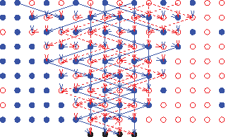
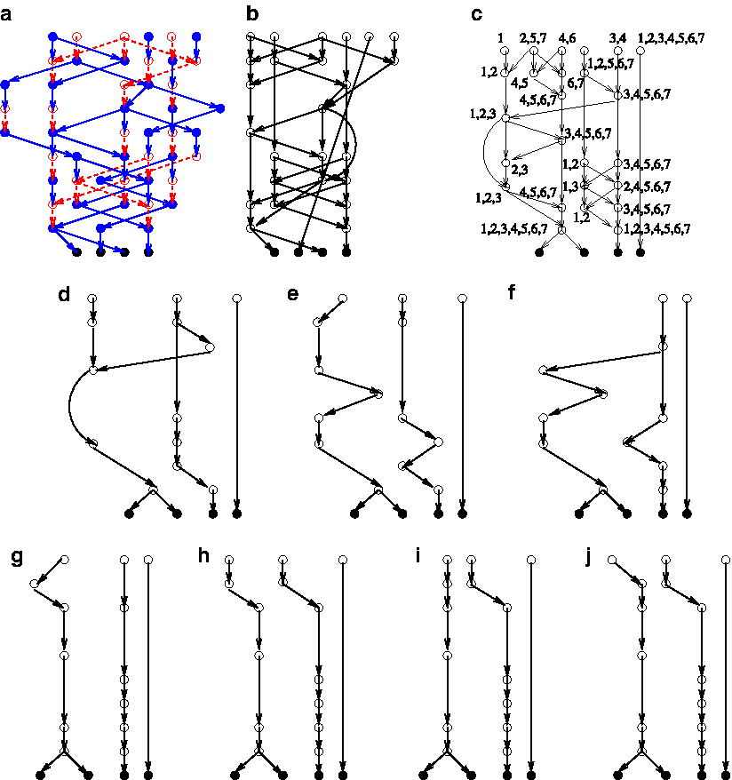
The first 10 generations of an instance of a relevant pedigree graph GPG(K,N) with K = 4 and N = 8. The solid (blue) dots represent one gender, say males and the hollow (red) dots represent the other gender (females). Each row is a generation with the direction on edges indicating the flow of the genetic material and the four extant units are at the bottom row, i.e., row 0. Under the Wright-Fisher Population model, there are equal number of males and females in each row, and the two distinct parents, one male and one female from the immediately preceding generation, are randomly chosen.
Vertices (K,N): The vertex set V is a countably infinite set. We suppose that the vertices are organized in rows, each of fixed size. Each row represents a generation and is numbered as
The vertex set in row 0 has K elements whose color is immaterial: these K nodes are also called the extant vertices.
The N vertices of each color in each row g can be labeled by a pair (g, j) where 1 ≤ j ≤ N. A graph instance is vertex-labeled if this label is associated with every vertex v of the graph instance.
Edges: All the edges in E are directed and are only between vertices of adjacent rows. Also, the direction of the edge is from the vertex at row g + 1 to the vertex at row g. Let
The parent vertex (vertices) is chosen at random reflecting the panmictic nature of the WF population. A parent and child are in adjacent rows due to the non-overlapping generations in the model (see Section 1). However, this can be easily relaxed to have overlapping generations and the essence of each discussion below still holds.
Note that one needs to distinguish between a specific instance or realization (sometimes called replica in the simulation parlance) of the random graph from the entity random graph itself which is a probability measure (to be specified later) on the space of infinite directed graphs with a countably infinite set of vertices. An instance of the random graph is obtained after executing the edge construction procedure as below.
Repeat for each row g: For each vertex u in row i, pick exactly one blue vertex v1 and exactly one red vertex v2 at random from row g + 1. The two directed edges are v1u and v2u.
Then,
Every instance of GPG(K,N ) is a directed acyclic graph (DAG). This follows from the fact that no vertex can be an ancestor of itself. An instance of GPG(K,N) corresponds to the entity termed pedigree graph in literature (Steel and Hein, 2006).
The number of vertices in row g is denoted by kg. Note that when g = 0, kg = K.
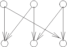
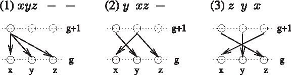
Can the pedigree graph be monochromatic? Forbidden structure in an instance of the pedigree graph. There exists no consistent assignment of red and blue colors (different genders) to the parents of the three vertices in the bottom row.
2.1. Least common ancestor (LCA)
The vertex set of an instance of the pedigree graph can be trimmed by focussing only on the flow of genetic information to the extant vertices. This is termed the relevant pedigree graph. A vertex va is an ancestor of vertex v if there exists a directed path from va to v. In graph-theoretic terms, it means that any vertex on the relevant pedigree must be an ancestor of at least one extant vertex. However, a relevant pedigree graph is also an infinite object. In the rest of the discussion, a pedigree graph is always a relevant pedigree graph.
A common ancestor va of vertices
Note that even though in every instance of the pedigree graph the indegree and outdegree of every vertex is bounded: indegree by 2 and outdegree by 2N and each row is bounded by 2N vertices, the number of possible LCA's might not be finite. Let Z(K,N ) be the random variable denoting the number of LCAs in GPG(K,N). Then
Moreover,
Lemma 1
1. There exist instances where Z(K,N) attains the value 0.
2. There exist instances where Z(K,N) attains the value ∞ .
Proof Sketch: We first prove the following two lemmas.
Lemma 2
Let vl at row g > 1 be an LCA.
(a) For an LCA v at row g′ > g, there exists no path from v to vl in the pedigree graph. (b) At every row g′ < g there exist at least two distinct vertices
Lemma 3
Let an LCA occur at depth gl with at least one LCA at a depth g′ < gl and with at least one LCA at a depth g″ > gl. Then row gl must have at least five vertices.
Corollary 1
For 1 ≤ N ≤ 2, there exists no instance with infinitely many LCAs.
Back to the proof of Lemma 1: Case 1: We construct an instance of the pedigree graph with no LCAs, i.e., Z(K,N) = 0. Let N ≥ 2. This construction is done in the following two steps. Let N = N1 + N2 and K = K1 + K2 with N1,N2 ≥ 1 and K1,K2 ≥ 1. In Step 1, construct an instance G1 of the pedigree graph GPG(K1,N1) and an instance G2 of the pedigree graph GPG(K2,N2). In Step 2, construct the union of the two graphs assuming that the two vertex sets are nonoverlapping (distinct labels in the two instances). It can be easily verified that this union is an instance of the pedigree graph GPG(K,N) and since it has at least two connected components, it has no LCAs.
Case 2: By Corollary 1, N > 2. We create an instance of the random graph GPG(4,3) that has an infinite number of LCAs, i.e., Z(K,N) = ∞ (Fig. 3). The construction is as follows. Row 0 has the four extant vertices. The outgoing edges from vertices in Row 0 and 1 are constructed as shown in the figure. The vertices in row 3 and higher are of three categories: (1) Two vertices of different colors called the blocked-vertices (two left vertices in the figure); (2) one vertex, called the LCA-vertex of any color (the middle vertex in the figure); (3) two vertices of the same color, but different from the color of the LCA-vertex called the path-vertices (two right vertices in the figure). The edge constructions follow a simple pattern as shown in the figure. Under this construction, the following can be verified: (1) the instance of the pedigree graph is valid, i.e., the color of the two parents of a node are of different colors, (2) every LCA-vertex of row 2 and higher is indeed the LCA of all the extant vertices.
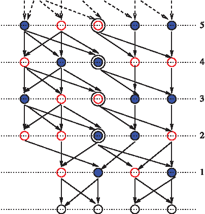
An instance of the pedigree graph GPG(4,3) (i.e., 4 extant vertices and population of size 3 for each gender at every generation) with an infinite number of LCAs. A possible coloring (or gender assignment) is shown for rows 1 and above; the colors of vertices of row 0 are immaterial. Only the first six rows are shown, marked from 1 to 5 (bottom row is 0). The LCAs are shown with an extra concentric ring. Rows 2 or higher: The block-vertices are the two leftmost vertices; the path-vertices are the two vertices in the right; the LCA-vertex is in the center. The same pattern of edges can be followed for all rows to define an infinite number of LCAs.
Corollary 2
For fixed parameters, K > 1 and N > 2,
1. there are infinite number of instances of GPG(K,N) each with no LCAs. 2. there are infinite number of instances of GPG(K,N) each with an infinite number of LCAs.
Next we make the assumption that any ancestor of an LCA is not of consequence and can be excised from the relevant pedigree graph. Is the pedigree graph after excising all the ancestors of all the LCAs finite? To summarize the answer to the question of finiteness of the excised pedigree graph with fixed parameters K(>1) and N(>2):
It is possible that an instance of the (excised) pedigree graph is infinite. Further, there are infinitely many such instances.
3. Pedigree Subgraphs
It is perhaps not very surprising to note that a pedigree graph may have multiple LCAs. However, it is rather surprising to note that even in a finite population model, the number of LCAs could be infinite (Lemma 1). This counter intuitive characteristic of the pedigree graph can be addressed by exploiting the biparental mode and coupling genetic exchange information with the topology of the pedigree graph.
Then, how about the parameter recombination rate ρ in a biparental model? Analogous to mutations (and other duplication-model genetic events), this should not affect the population dynamics but only the sequences of the units. Again, it is (by current biotechnologies) not a direct observable but can be inferred from the sequences in the population. However, just as in the unilinear transmission model, the vertices that have no paths to an extant unit is not relevant for the study, so in the biparental model, vertices that have no genetic material ancestral to any in the extant units are not of relevance. The definition of the relevant pedigree graph is now extended to exclude those vertices that do not carry any genetic material to the extant units (although there may be a path in the graph to an extant vertex). It now seems more natural to annotate the vertices of the biparental graph with the nonmixing segments (i.e., a segment that is inherited completely from the mother or the father but not mixed by the two parents) of genetic materials. Thus, instead of ρ, a more natural parameter seems to be M, the number of nonmixing units in the extant population. We claim that the parameter M models the biparental mode as a natural extension of the (well-accepted) unilinear transmission mode and ρ continues to be “external” to the population.
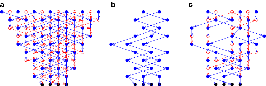
We identify two classes of subgraphs of the pedigree graph GPG(K,N) as our objects of study (Fig 4. shows the different subgraph models of the pedigree graph):
1. Unilinear Transmission: A monochromatic subgraph GPT(K,N) is induced on the vertices of one color (either only blue or only red). Thus each vertex has exactly one parent. The biological interpretation of a monochromatic subgraph is as follows. The genetic material that is transmitted only through the blue vertices (father) is the nonrecombining Y chromosome (NRY). Similarly, the genetic material that is transmitted only through the red vertices (mother) is the mitochondrial DNA. These subgraphs of the pedigree graph actually represent the duplications-only model. Lemma 5 has an interesting consequence: All the genetic material in the extant sequences can be traced back to a unique vertex in the pedigree graph. Topologically, this vertex is the LCA and is called the most recent common ancestor (TMRCA). 2. Genetic Exchange Model: In this model, genetic material is additionally associated with the vertices. M is an upper bound on the number of non-mixing (or genetic exchange) segments in the extant units, which is used as an additional parameter. A mixed subgraph GPGE(K,N,M) is induced on some blue and some red vertices. Thus the vertices have may have either one or two parents. Lemma 7 has an interesting consequence: All the genetic material in the extant sequences can be traced back to a unique vertex in the pedigree graph. Topologically, this vertex is the LCAA (defined in Section 3.2.1). This is called the grand most recent common ancestor (GMRCA).
3.1. Unilinear transmission: monochromatic subgraphs G PT (K,N)
Mutation events or genetic events such as the ones leading to Short Tandem Repeat (STR) polymorphisms are modeled as duplication events or simply non-recombining events (Hein et al., 2005; Jobling et al., 2004). Hence, this is also called the duplications-only model and each vertex has only one parent. Since we do not model any gender-specific characteristics, the duplications-only model is equivalent to the monochromatic (all vertices of the same color) model in our general setting. The following is easily verified.
Lemma 4
The monochromatic subgraph is a forest (tree), i.e., the graph has no closed paths.
Hence the monochromatic subgraph is written as GPT(K,N).
Lemma 5
Given an instance of a monochromatic subgraph GPT(K,N):
1. The number of vertices can neither increase with depth nor be zero at any row, i.e.,
2. The number of LCAs is at most 1.
(kg = 1) ⇔ The vertex at row g is the LCA.
Proof Sketch: 1. This follows from the fact that the graph is a tree. 2. Assume the contrary that an instance has l > 1 LCAs. Let v1 and v2 be two distinct LCAs. Then there must exist vertices u1 and u2 (possibly with u1 = u2) where u2 is an extant vertex and there is a path from v1 to u1, a path from v2 to u1 and a path from u1 to u2. Further let u1 be such that there is no other vertex u′ with a path from v1 to u′, v2 to u′ and u′ to u1 (if such is the case then we call u′ as u1). Observe that each vertex of the monochromatic subgraph has at most one parent. However, u1 must have at least two parents (each on the two distinct paths to the two LCAs v1 and v2) contradicting this fact. Hence the assumption must be wrong and the number of LCAs l ≤ 1. 3. This follows from 2.
Corollary 3
For fixed parameters, K > 1 and N ≥ 1, there are infinitely many monochromatic subgraphs with no LCAs.
3.2. Genetic exchange model: mixed subgraph G PGE (K,N,M)
Given K extant sequences, the most recent common ancestor (MRCA) is a sequence S from some generation such that the genealogy of every segment (nucleotide) of every extant sequence can be traced back to S. Further, amongst all such common ancestors, S is the most recent one. In population genetics, usually the term MRCA is used for the duplications-only model, and the term grand MRCA (GMRCA) is used when the genetic events include rearrangements of the sequence, such as recombinations (Hein et al., 2005). In the following, we use M, an upper bound on the number of mixing segments in the extant units, to parameterize a general genetic exchange model. A Mixed Subgraph GPGE(K,N,M) is defined as follows. For each instance G of the mixed subgraph:
Each vertex in G is annotated with M nonmixing segments and must have genetic material that flows to at least one of the extant vertices. This implies that a vertex may have only one parent (if the other parent has no genetic material flowing to an extant unit). Each genetic mixing event is equally likely to occur. This is only a simplifying assumption and in the same spirit as random mating or panmictic condition of the Wright Fisher population. A deviation from this assumption can be handled quite simply by modifying the set definitions in Section 6.3.2.
The flow of the genetic material gm(e) through an edge e and the genetic material gm(v) of a vertex v are not independent and are related by the two rules.
Rule 1: Let u be a vertex with d ascendant (incoming) edges ei,i = 1.d (the valid values of d are 1 or 2).
(Note that S = S1 ∐ S2 denotes that S is the disjoint union of S1 and S2, i.e., S1 ∩ S2 = ∅.) Rule 2: Let v be a vertex with d descendant (outgoing) edges ei,i = 1.d.
Let m graphs Gi(Vi,Ei) with vertex set V
i
and edge st Ei be defined on (labeled) vertices, 1 ≤ i ≤ m. Then the induced graph on vertices
Lemma 6
Given G, an instance of a mixed subgraph GPGE(K,N,M), the following hold.
1. For each vertex v and each edge e of G,
2. Let (a) Tm is a forest for all 1 ≤ m ≤ M. (b)
3. Let the set of vertices at depth g be Vg. The following holds for each depth g.
(a) |Vg| ≤ KM. (b) For each nonmixing unit 1 ≤ m ≤ M,
Proof Sketch: (1) This follows from the definition of the mixed subgraph (each node must have genetic material that flows to at least one extant vertex). (2a) Assume that the result is not true: For some m, Tm has a closed path. By the nature of the direction of the edges in the pedigree graph, then there exists a vertex v with two distinct paths P1 and P2 to u. Without loss of generality, let the two paths be nonintersecting, except at v and u. Clearly, by Rule 1, the two incoming edges e1 and e2 on u cannot be such that
Thus
Hence, the result. (3a, 3b) In each Tm the number of vertices per row does not exceed K. Also, each vertex in Tm must be annotated with the genetic element m. Thus, by 2(b), the number of vertices in G cannot exceed KM and the number of nodes with nonmixing element m cannot exceed K.
See Equation 1 for all possible gm annotations for some fixed values of M,K,kg. An example is shown in Figure 5 of the embedded trees in an instance of a mixed subgraph. An instance of a graph where each vertex v has genetic material gm(v) defined is said to be gm-annotated. Note that in a monochromatic subgraph, for any two distinct vertices v1 and v2, gm(v1) = gm(v2). Thus, a monochromatic subgraph can be considered to be always gm-annotated. Also we write the gm annotation of vertex vi simply as
(instead of gm(vi)). Also if vertex vi is in row g, the annotation may be also written as
3.2.1 Topological definition of GMRCA: least common ancestor with ancestry (LCAA)
Conceptually the term LCA is equivalent to MRCA. However, LCA is not equivalent to GMRCA, which additionally is also ancestral to the genetic material in the extant vertices. This is due to the following fact: If node va is an ancestor of some node v in GPG(K,N), then it is possible that not all the genetic material of va is ancestral to the genetic material of v. It is also possible that va is ancestral to no genetic material of v. In the latter case a topological ancestor is not a “genetic” ancestor. For example, see Figure 6. A natural question is if there exists a purely topology-based definition that captures the notion of a GMRCA. We call this the LCA with ancestry or LCAA, a graph-theory based term for the GMRCA (it is defined in the lemma below). Given G an instance of a mixed subgraph GPGE(K,N,M), by Lemma 6, let
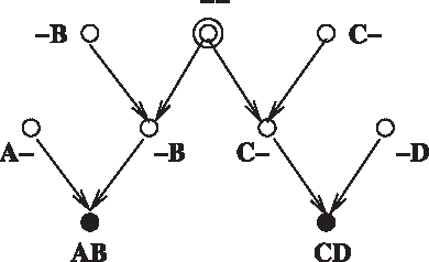
Ancestor without ancestry: Each node is annotated with the genetic material labeled as a combination of
Then,
Lemma 7
1. The following two definitions of LCAA are equivalent:
(a) (population genetics based) the least, or most recent, common ancestor of the K extant units that is also ancestral to all the genetic material in the K units.
(b) (graph-theory based) the LCA of the LCA's of
2. The number of LCAAs is at most 1.
3. (kg = 1) ⇔ The vertex at row g is the LCAA.
Proof Sketch: We prove the second statement first. 2. Let every genetic unit (say a nucleotide) be tagged by a two tuple, its position in the chromosome and the label of extant vertex. Thus, assuming there are c nucleotides and K extant units, there are cK distinct tuples. Next the genetic flow from vertex to vertex through the edges is marked by the tuples. It is easy to see that a path marked with a specific tuple is a chain (that does not branch). Thus, if vertex v is a GMRCA, then by definition, v is on all the cK paths. Thus there cannot exist more than one GMRCA since all the marked paths are chains. 1. Let v″ be the LCAA by definition (a). Note that in tree, Tm, 1 ≤ m ≤ M, the LCA of Tm, say vertex vm, is also the LCAA of the extant units, corresponding to genetic material m. Further let v′ be the LCA of
Lemma 8
The effective value of M for a pedigree graph with N blue or red vertices at some depth is:
4. Probability Space of (Infinite) Pedigree Subgraphs: Uniform Distribution on [0,1]
In this section, we address the problem of mapping the instances of the pedigree graph to a measurable space with the goal of defining a natural probability space. The Wright-Fisher population model suggests a uniform probability space as an appropriate choice. The treatment of the models, monochromatic and mixed subgraphs, are very similar and to avoid repetition of the arguments in the following discussion, all the models are treated simultaneously. Our definition of the probability measure is inspired by (and along similar lines to) the classical construction of finitely additive, invariant measures on infinite groups such as the integers using Følner (1955) sequences.
Note that the set of graph instances is not enumerable (this can be seen by a mapping of the instances to the reals). To enable computations, let the graph have a fixed height h (>1), i.e., a finite number of generations. Now, since the graph is finite, the instances are finite. The limit as h → ∞ gives us a basis for defining a probability space (details in Section 4.2).
4.1. Fixed depth subgraphs
Let
where
For sufficiently large h, Lh = L, where
In order to compute and enumerate all the configurations, we define the following set-valued functions.
Recall that N is the the number of vertex-labeled vertices in every row. Thus for k vertices at any row, define a function, which we call the weight function, as follows (see Example 5 for illustrations):
The numbers (cardinalities) associated with each of the set-valued functions are as follows. For h ≥ 1,
Example 1
(on
Example 2
(on
To avoid clutter, in the following Q2( · , · ) is written simply as Q( · , · ). Thus,
Mixed subgraph model.
Condition (1) ensures that every vertex in row g has at least one parent (in row g + 1); condition 2(a) states a vertex with more than one nonmixing unit associated with it, could have at most two parents; condition 2(b) states that the genetic material is split between the parent(s); condition (3) states the condition where a vertex can have only one parent. Further details are presented in Section 6.3.2.
Monochromatic subgraph model.
Condition (1) ensures that every vertex in row g has a parent (in row g + 1); condition (2) ensures that no vertex has more than one parent. Further details are presented in Section 6.3.1.
Back to
Also,
Lemma 9
For all kg and kg+1,
4.1.1. Equivalence classes
We identify isomorphic graphs, i.e., the graphs that are isomorphic after forgetting the labels, but not the color. Recall that kg is the number of vertices at row g of
See Figure 7 for an example of the forgetful graphs. Let
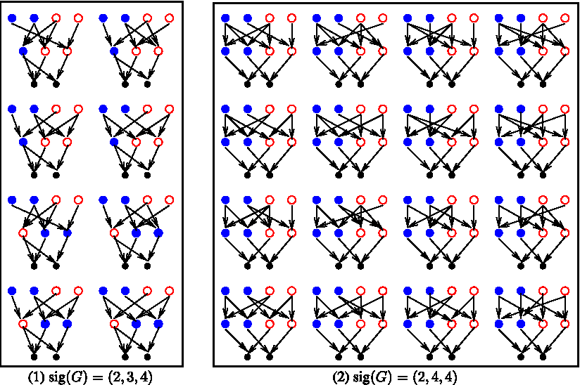
To limit the number of equivalence classes, here we focus only on the ones where no vertex has only one parent. Then with K = 2, N = 2 and depth h = 2, the equivalence classes are shown with the unlabeled, forgetful member graphs.
To aid in computing the expected location of LCAA in the models, we also define
4.2. Measurable space
The Wright-Fisher model implies every instance of the vertex-labeled (and additionally, gm-annotated in the genetic exchange model) graph is equally likely to occur. We make a few remarks about the underlying probability measure on
Each instance of the (infinite) graph is mapped to a real number in the interval [0,1]. More precisely, there exists a bijection
which has the property that
using Eqns 2 and 4. Then the following holds.
Lemma 10
For each h > 0,
Then the uniform probability measure μ on
where for any
For some (event)
Suppose that
Then,
Lemma 11
Using the bijection ϕ,
Thus
Since each
5. Reconstructability of Pedigree History
Usually simplifying assumptions about genetic events (say mutations, recombinations) such as infinite-sites model (Kimura, 1969) or infinite-alleles model (Kimura and Crow, 1964) are made, either from a reconstructability or a modeling perspective. The former model implies that any two events at different points in time (generations) do not occur at the exact same location on the sequence. In a similar spirit, the latter model permits multiple mutations at a location but each produces a unique allele. Thus the models avoid recurrent events at the same location which can be distracting for a framework that is grappling with the inference of reconstructing the history—the identification and time ordering (over generations) of all the genetic events in all the sequences. However, recurrence of genetic events is observed in nature (called back mutations, parallel mutations, recombination hotspots and so on). Nevertheless, these models are reasonable and are widely accepted. Also, note that the HUD (Wiuf and Hein, 1999a) is a more restrictive ARG model, with a view to reconstructability. These restrictions can be translated to topological properties, such as galled trees and related graph theoretic ideas (Gusfield et al., 2007).
However, we take a much less conservative view: here we simply use the size of the pedigree history structure as a measure of reconstructability. A large structure is hard to reconstruct whereas a small structure is more amenable to faithful reconstruction (also a network is harder to reconstruct than a tree). Let the LCAA occur at depth g for an instance of the graph. The size is parameterized by the depth of the LCAA, since the vertices at a deeper depth (or at row > g) are not informative either for ancestry or reconstruction purposes. For this end, we compute the expected depth of the LCAA in both the subgraph models.
5.1. On LCAA probabilities
By Lemmas 5 and 7 if the number of LCAAs < ∞ in an instance of the mixed or monochromatic subgraph model, then it is a singleton vertex in some row of the instance. Consider Eqn. 9: F( · , · ) satisfies the following for 1 ≤ k ≤ L (see Eqn. 2 for L) and g > 1.
5.1.1. Common Ancestor with Ancestry (CAA)
Lemma 12
In a relevant pedigree graph (for both models),
1. if there exists a CAA at depth g, then the same is true for all g′ ≥ g, and, 2. if there exists no CAA at depth g, then the same is true for all g′ ≤ g.
Further, using Lemmas 5 and 7, the probability of a common ancestor with ancestry at depth h of a graph
Monochromatic Subgraph Model. To get a workable form of F(g), it is convenient to expand Eqn. 12 for monochromatic models as:
Then,
Mixed Subgraph Model. Expand Eqn. 12 for mixed subgraph models as:
Back to Computations. Then for both models (see Eqn. 18 in Appendix),
5.1.2. Least Common Ancestor with Ancestry (LCAA)
Next we explore the event of the the common ancestor at depth h being the most recent as well, i.e., additionally there is no common ancestor below the depth of h. Recall that the LCAA for the monochromatic subgraph is just the LCA. We handle both the cases together. Let
By Lemma 12, the event of occurrence of the LCA at depth h is not independent of the occurrence at h′ ≠ h. This dependence is captured in the following. Let F1(h) be the number of instances in
Also note that,
Then for all h ≥ 1,
5.2. Expected depth
\documentclass{aastex}\usepackage{amsbsy}\usepackage{amsfonts}\usepackage{amssymb}\usepackage{bm}\usepackage{mathrsfs}\usepackage{pifont}\usepackage{stmaryrd}\usepackage{textcomp}\usepackage{portland, xspace}\usepackage{amsmath, amsxtra}\pagestyle{empty}\DeclareMathSizes{10}{9}{7}{6}
\begin{document}
$${\mathbb E} \left[D \right]$$
\end{document}
of LCAA
Let D be a random variable that denotes the depth (row or generation) of an LCA. Then
Using Eqn. 14, the sum on the right is:
where
Using the identity, for |x| < 1,
for both models we have,
Assuming that the tree (monochromatic subgraph), of expected depth ≥ Ω(NK), is reconstructible, we conclude that a mixed subgraph can be reconstructed when M is small. In other words, for a given set of extant sequences, the joint history of local segments along a chromosome is reconstructible.
6. Sampling The Space of Pedigree Subgraphs
Here we address the problem of random generation of the combinatorial structure of a pedigree subgraph (monochromatic or mixed). Here we weave the combinatorial arguments, presented earlier in this article, together into a random-instance construction algorithm. While approximate distribution functions can be used for computational efficiency, it is important to note that the only parameters that define the random instance of the mixed subgraph are K, N, and M, and the defining parameters for a monochromatic subgraph are K and N.
6.1. Sampling algorithm
We use two parameters gmax, the maximum number of generations and Kmin, the minimum number of units per generation as a stopping criterion, for a loop that is theoretically infinite (since an instance may not have any LCAAs by Corollary 3). The random instance is constructed by the configurations that are defined at each step. For an example of interpreting a configuration encoding, see Figure 8.
Interpreting the encodings:
In the pseudocode, we use the following conventions: (1) Assignment: “Y ← y” is to be interpreted as variable Y being assigned the value y. (2) Autoincrement: “++ g” is to be interpreted as the variable g being first incremented by 1 before using it. (3) Loop: “REPEAT .code. UNTIL (condition)” is to be interpreted as repeating the code until the condition is satisfied. The rest should be clear from context.
The functions
6.2. Algorithm property
(Monochromatic subgraph model GPT(K,N)
Mixed subgraph model GPGE(K,N,M)
Further, the associated numbers of the sets (cardinalities) used in the algorithm are:
(see Examples 3–8 for illustrations of the combinatorial sets).
6.3. Constructing local configurations between rows g and g + 1
Given a monochromatic model or a mixed model, Q(kg,kg+1) is the number of distinct vertex-labeled and gm-annotated configurations between rows g with kg vertices and g + 1 with kg+1 vertices. The following gives illustrative examples for all the sets and functions involved in their enumeration or computation.
6.3.1. Vertices in row g with 1 parent
Consider two adjacent rows g and g + 1 with kg vertices in row g. When a vertex always has exactly one parent, the vertices in row g + 1 can be considered to be monochromatic (for computational purposes).
Example 3
(on
Example 4
(on
To avoid clutter the set of sets notation is simplified: for example the set
is written simply as
Then the 45 elements of
Example 5
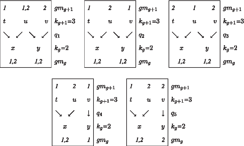
(on wt(k) function). Let kg = 3 and X = {x,y,z}. Let qc = 1 ≤ 2, with qd = ({x},{y,z}), i.e., kg+1 = 2. Let N = 4. Then the number of possible configurations is
The weight 6 corresponds to the 6 configurations shown below with the labels of row g + 1 implicit by their position (first, second, third or fourth):
Note that for qd = ({y, z}, {x}), the 6 possibilities are:
6.3.2. Vertices in row g with 1 or 2 parents.
Example 6
(on
Thus S1 = {y}, S2 = {x,z}. Cardinality of C must satisfy the following:
Thus the three possible C's are: C1 = {x},C2 = {z},C3 = {x,z}.
Case C1 = {x}: Let S3 = (S2 \ C) ∪ S1 = {y,z}. The possibilities are:
Case C2 = {z}: Let
Case C3 = {x, z}: Let S3 = (S2 \ C) ∪ S1 = {y}. The possibilities are:
Thus for the gm defined in this example,
Example 7
(on
Thus, of the three vertices labeled x, y, z in some row g, only vertex y has one parent and the other two have two parents each in row g + 1. In the following we use the simplified notation of the configuration of Example 4. Then
where
Example 8
(on  denote a descendant edge from a blue vertex in row g + 1 to a vertex in row g and
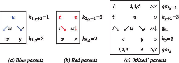
  denote a descendant edge from a red vertex in row g + 1 to a vertex in row g. The genetic segments in gm( · ) is displayed next the vertices (x, y, z in row g) and the edges in the examples below. Consider the following configuration:
The different possibilities of genetic material assignment to the vertices with two parents is shown here.
(1)–(4) model recombination event and (5)–(6) model gene conversion event at node labeled x. Then the (unique) gmg+1 annotation for case (1) above shown in (c) below with labels of vertices in row g + 1 as {t,u,v} (for convenience, incident edges on blue parents is shown in blue in (a) and incident edges on red parents is shown in red in (b)):
Note that handling blue and red parents separately ensures that there are no forbidden structures (Fig. 2) between rows g and g + 1.
7. Discussion
In conclusion, we have presented a unified random graphs framework to study pedigree history with focus on unilinear transmission trees and the biparental transmission ARGs, the two interesting mathematical objects in this context. In the unified framework, the two are modeled as monochromatic and mixed subgraphs respectively of the pedigree graph. In the former, each vertex has no more than one parent with all vertices of the same color (gender). In the latter, each vertex has one or two parents, dictated by genetic exchange and subsequent flow of the genetic material through the nodes to the extant units. One of the interesting consequences of this approach is a pure topological definition of the GMRCA (called LCAA to be analogous with the graph-theoretic LCA). This is the first time that an ARG as well as the GMRCA are given a graph-theoretic description with an alternative parametrization of the ARG. The article also identifies a natural measure space, which then helps estimate the expected depth of an LCAA in a pedigree graph/ARG/unilinear transmission tree.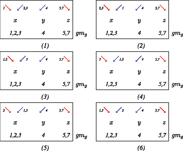
The sampling algorithm presented in this article is a rather straightforward and direct application of the ideas used in defining the measurable space. It will be quite interesting to adapt the ideas to a coalescent (Hudson, 1990; Kingman, 1982) version of the algorithm that continues to guarantee uniform sampling of the ARG space. Yet another direction is the incorporation of selection, random environment variables, or other such (biasing) dynamics into the ideal population. The study of the effect of these on the topology, including LCAA depth, and scattering patterns of the genetic material over the vertices in the subgraph models, as well as design of sampling algorithms under these conditions, are interesting directions of exploration.
8. Appendix: A Mixed Subgraph Model
See Section 4 for the definitions used here. Let
Note that when M = 1 (monochromatic model), for all possible values of
For
Then
Lemma 13
Thus for the mixed model,
Also (see Eqn 13),
Footnotes
Acknowledgments
This work would not have been possible without the indulgence and support of experts from different fields. I am thankful to Jaume Bertranpetit (and colleagues) for sowing the seeds of skepticism that motivated the study. I am indebted to Jotun Hein, Paul Marjoram, and Carsten Wiuf for useful discussions on the population models and help distill my thoughts on their stochasticity and implications. I am very grateful to David Sankoff and Saugata Basu for enlightening discussions on measure theory. Also, many thanks go to Asif Javed and Ajay Royyuru for reading a preliminary version of the manuscript.
Disclosure Statement
No competing financial interests exist.