The current methods for the determination of the statistical significance of peaks and regions in next generation sequencing (NGS) data require an explicit normalization step to compensate for (global or local) imbalances in the sizes of sequenced and mapped libraries. There are no canonical methods for performing such compensations; hence, a number of different procedures serving this goal in different ways can be found in the literature. Unfortunately, the normalization has a significant impact on the final results. Different methods yield very different numbers of detected “significant peaks” even in the simplest scenario of ChIP-Seq experiments that compare the enrichment in a single sample relative to a matching control. This becomes an even more acute issue in the more general case of the comparison of multiple samples, where a number of arbitrary design choices will be required in the data analysis stage, each option resulting in possibly (significantly) different outcomes. In this article, we investigate a principled statistical procedure that eliminates the need for a normalization step. We outline its basic properties, in particular the scaling upon depth of sequencing. For the sake of illustration and comparison, we report the results of re-analyzing a ChIP-Seq experiment for transcription factor binding site detection. In order to quantify the differences between outcomes, we use a novel method based on the accuracy of in silico prediction by support vector machine (SVM) models trained on part of the genome and tested on the remainder. See Kowalczyk et al. (2009) for supplementary material.
1. Introduction
Current short read sequencing technology, routinely referred to as next generation sequencing (NGS), allows for genome wide scans for various phenomena of interest, such as methylation and transcription factor binding sites. In order to derive meaningful results from the mapping of short reads (or tags) to the reference genome, a number of statistical filters based on the binomial distribution, Poisson distribution and their variants have been proposed in the literature (Rozowsky et al., 2009; Nix et al., 2008; Robertson et al., 2007; Kowalczyk, 2009). These methods are also very similar to SAGE data analysis (Baggerly et al., 2003; Robinson and Smyth, 2007), which also deals with short sequence data.
In order to discern a meaningful signal from tags mapped to a reference genome, a number of biases have to be dealt with and corrected for, as the signal “is actually the convolution of a number of effects: the density of mappable bases in a region, the underlying chromatin structure and the actual signal from transcription factor binding” (Rozowsky et al., 2009). The natural way to mitigate these issues is to introduce control samples, so that the detected signal is in the form of local enrichment of tag counts with respect to the control. The closer the preparation and processing of the control to the target sample, the more reliable the mitigation of biases.
However, experimenters cannot ensure that the target and control samples are prepared and processed in a completely equivalent manner and in practice the number of tags derived from two separate sequencing reaction can differ by a significant factor. This situation becomes endemic if one attempts to develop local models (Rozowsky et al., 2009), compensating for local biases along the reference DNA. In the simplest situation such as ChIP-Seq experimental detection of binding sites for a transcription factor (Rozowsky et al., 2009), where one attempts to detect enrichments in the target sample with respect to a carefully prepared control, there is a plausible argument for scaling the control sample counts to the level of the target, especially when considering pre-filtered narrow regions of significant enrichment.
In practice, there are other scenarios where such scaling is less applicable. An example is where one looks for the differential peaks between two different tissue samples, for example, differences in methylation between two cell lineages (Bloushtain-Qimron et al., 2008; Kowalczyk, 2009). Here, even the direction of scaling (local or global) is not obvious. Moreover, as argued in Kowalczyk (2009), the common level to which the sample counts are adjusted has a profound impact on the statistical significance of peaks when either Poisson or binomial models are used (see Section 3.3); thus, the number of detected peaks depends significantly on the choices of scaling strategies.
The situation becomes even more cumbersome for experiments that involve multiple samples, for example, when quantifying the difference between two cell lineages using pairs of samples collected from multiple subjects in order to account for patient specific heterogeneity. One possibility is to adjust all counts to a common size across the whole collection. As we have noted, this common size impacts on the number of “significant peaks” as in practice scaling could be by a factor of 2 or more with the resulting variation in p-values being by a factor of 4 or more. Moreover, the addition of new samples to the analysis could lead logically to readjustment of the updated “common size” distorting the previous results. The ad hoc nature of some of these adjustments undermines the principled statistical analysis, introducing arbitrary design choices and obscure data driven adjustments.
In this article, we propose a different statistical technique that does not require an explicit sample size adjustment and thus functions directly on the original counts. Any adjustments can be used as an additional means for accounting for other biases in the data. An example of this is the known variations in the density of mappable tags (i.e., the effective depth of sequencing) (Rozowsky et al., 2009) along the DNA sequence.
2. Background
We now outline a conceptual model that can be used while reading this article. Using a specific protocol (e.g., sonication, enzymatic reactions cutting the DNA at specific locations, protein immunoprecipitation selecting specific fragments of protein bound to them), a library L of DNA fragments is prepared. From this library, a subset R is randomly sampled, and for each of the sampled fragments a part of it, a short read, is sequenced providing a tag, which is a k-mer of DNA bases. The tag is then mapped to one or many matching locations in an a priori known reference DNA sequence, the human genome in our case, using a specific protocol, for example, only exact matching, or only exact and unique, or only unique with up to one error. We are interested in the reference genome locations where significant over/under-representation of the mapped tags occur, so called peaks or peak ranges, as these can be interpreted as evidence for some specific property of DNA or its epigenetic modifications. In some experiments such as SAGE-Seq or digital karyotyping (Bloushtain-Qimron et al., 2008; Kowalczyk, 2009), there are natural peak regions, as the tags congregate at specific DNA locations determined by the enzymes used to cut the source DNA. In other cases, such as ChIP-Seq experiments using sonication, the peak regions have to be determined from the data using specific algorithms (Rozowsky et al., 2009; Zang et al., 2009), or perhaps just defined by a simple partitioning of the genome into uniform small blocks, say, on the order of a thousand bases.
In this section, we assume that a set of peak regions of interest is given to us. Let us consider a single peak range r. We denote by X = X(R) a random variable of the count of tags mapped to r, and by x its particular realisation. If we denote by λ, 0 < λ < 1, the proportion (fraction) of reads in the library L with tags mappable to r, then X can be modelled as a binomial random variable, Bin(λ, |R|):
\documentclass{aastex}\usepackage{amsbsy}\usepackage{amsfonts}\usepackage{amssymb}\usepackage{bm}\usepackage{mathrsfs}\usepackage{pifont}\usepackage{stmaryrd}\usepackage{textcomp}\usepackage{portland,xspace}\usepackage{amsmath,amsxtra}\pagestyle{empty}\DeclareMathSizes{10}{9}{7}{6}\begin{document}\begin{align*}
{\mathbb P} [x = X (R)] = {{\mid R \mid} \choose {x}} \lambda^x (1
- \lambda)^{\mid R \mid - x} , \tag{1}
\end{align*}\end{document}
for \documentclass{aastex}\usepackage{amsbsy}\usepackage{amsfonts}\usepackage{amssymb}\usepackage{bm}\usepackage{mathrsfs}\usepackage{pifont}\usepackage{stmaryrd}\usepackage{textcomp}\usepackage{portland,xspace}\usepackage{amsmath,amsxtra}\pagestyle{empty}\DeclareMathSizes{10}{9}{7}{6}\begin{document}$$x = 0 , 1 , \ldots , \mid R \mid$$\end{document}. In a typical case of interest λ ≪ 1 and the distribution of X is very well approximated by the Poisson distribution (Keeping, 1995), Poi(μ):
\documentclass{aastex}\usepackage{amsbsy}\usepackage{amsfonts}\usepackage{amssymb}\usepackage{bm}\usepackage{mathrsfs}\usepackage{pifont}\usepackage{stmaryrd}\usepackage{textcomp}\usepackage{portland,xspace}\usepackage{amsmath,amsxtra}\pagestyle{empty}\DeclareMathSizes{10}{9}{7}{6}\begin{document}\begin{align*}
{\mathbb P} [x = X] = \mu^x \frac {e^{- \mu}} {x!} , \tag {2}
\end{align*}\end{document}
where \documentclass{aastex}\usepackage{amsbsy}\usepackage{amsfonts}\usepackage{amssymb}\usepackage{bm}\usepackage{mathrsfs}\usepackage{pifont}\usepackage{stmaryrd}\usepackage{textcomp}\usepackage{portland,xspace}\usepackage{amsmath,amsxtra}\pagestyle{empty}\DeclareMathSizes{10}{9}{7}{6}\begin{document}$$x = 0 , 1 , \ldots , \mid R \mid$$\end{document} and the Poisson rate is defined as μ = λ|R|.
3. The Poisson Margin Test
Now we focus on comparing two libraries, LA and LB, from which random samples of mappable tags RA and RB were drawn, respectively. Suppose we have observed counts xA and xB of tags mapped to the specific peak range r of interest, and λA and λB are the corresponding proportions of tags in the libraries LA and LB mappable to r, respectively. Let \documentclass{aastex}\usepackage{amsbsy}\usepackage{amsfonts}\usepackage{amssymb}\usepackage{bm}\usepackage{mathrsfs}\usepackage{pifont}\usepackage{stmaryrd}\usepackage{textcomp}\usepackage{portland,xspace}\usepackage{amsmath,amsxtra}\pagestyle{empty}\DeclareMathSizes{10}{9}{7}{6}\begin{document}$$(a , b) \in \{(A , B) , (B , A) \} $$\end{document} and the following relation for empirical proportions holds:
\documentclass{aastex}\usepackage{amsbsy}\usepackage{amsfonts}\usepackage{amssymb}\usepackage{bm}\usepackage{mathrsfs}\usepackage{pifont}\usepackage{stmaryrd}\usepackage{textcomp}\usepackage{portland,xspace}\usepackage{amsmath,amsxtra}\pagestyle{empty}\DeclareMathSizes{10}{9}{7}{6}\begin{document}\begin{align*}
\hat {\lambda}_a : \ = \frac {x_a} {\mid R_a \mid} < \hat {
\lambda}_b : \ = \frac {x_b} {\mid R_b \mid} . \tag {3}
\end{align*}\end{document}
How strong is this evidence for λa < λb? We approach this issue in a typical statistical hypothesis testing manner. Namely, we are interested in testing the alternative hypothesis (H1) that λa < λb versus the null hypothesis (H0) that λa ≥ λb, i.e., that the complementary relation holds. As a natural test statistic we can use the maximal probability of observing at least as extreme counts Xa,Xb under the null hypothesis (H0). This probability we shall quantify in two different ways, a test based on the binomial distribution (Binomial Margin, \documentclass{aastex}\usepackage{amsbsy}\usepackage{amsfonts}\usepackage{amssymb}\usepackage{bm}\usepackage{mathrsfs}\usepackage{pifont}\usepackage{stmaryrd}\usepackage{textcomp}\usepackage{portland,xspace}\usepackage{amsmath,amsxtra}\pagestyle{empty}\DeclareMathSizes{10}{9}{7}{6}\begin{document}$${\cal M}_{Bi}$$\end{document}) and its Poisson approximation (Poisson Margin,\documentclass{aastex}\usepackage{amsbsy}\usepackage{amsfonts}\usepackage{amssymb}\usepackage{bm}\usepackage{mathrsfs}\usepackage{pifont}\usepackage{stmaryrd}\usepackage{textcomp}\usepackage{portland,xspace}\usepackage{amsmath,amsxtra}\pagestyle{empty}\DeclareMathSizes{10}{9}{7}{6}\begin{document}$${\cal M}_{Po}$$\end{document}), respectively:
\documentclass{aastex}\usepackage{amsbsy}\usepackage{amsfonts}\usepackage{amssymb}\usepackage{bm}\usepackage{mathrsfs}\usepackage{pifont}\usepackage{stmaryrd}\usepackage{textcomp}\usepackage{portland,xspace}\usepackage{amsmath,amsxtra}\pagestyle{empty}\DeclareMathSizes{10}{9}{7}{6}\begin{document}\begin{align*}
\begin{split}
{\cal M}_{Bi} (x_a , x_b) : \ = \sup_{\lambda_a \geq \lambda_b >
0}{\mathbb P} \left[X_a \leq x_a \ \& \ x_b < X_b \ \big | \ X_i
\sim Bin (\lambda_i , | R_i |) \right] , \\ {\cal M}_{Po} (x_a ,
x_b) : \ = \sup_{\lambda_a \geq \lambda_b > 0}{\mathbb P}
\left[X_a \leq x_a \ \& \ x_b < X_b \ \big | \ X_i \sim Poi (
\lambda_i | R_i |) \right] , \end{split} \tag{4}
\end{align*}\end{document}
In practice, both tests are numerically equivalent, but \documentclass{aastex}\usepackage{amsbsy}\usepackage{amsfonts}\usepackage{amssymb}\usepackage{bm}\usepackage{mathrsfs}\usepackage{pifont}\usepackage{stmaryrd}\usepackage{textcomp}\usepackage{portland,xspace}\usepackage{amsmath,amsxtra}\pagestyle{empty}\DeclareMathSizes{10}{9}{7}{6}\begin{document}$${\cal M}_{Po}$$\end{document} is easier to handle analytically and computationally, and will be the primary focus of the rest of this article.
We observe that the above definitions do not require that the sample sizes |RA| and |RB| be equal. By definition, the Poisson margin \documentclass{aastex}\usepackage{amsbsy}\usepackage{amsfonts}\usepackage{amssymb}\usepackage{bm}\usepackage{mathrsfs}\usepackage{pifont}\usepackage{stmaryrd}\usepackage{textcomp}\usepackage{portland,xspace}\usepackage{amsmath,amsxtra}\pagestyle{empty}\DeclareMathSizes{10}{9}{7}{6}\begin{document}$${\cal M}_{Po}$$\end{document} is the tightest universal upper bound on the following probability
\documentclass{aastex}\usepackage{amsbsy}\usepackage{amsfonts}\usepackage{amssymb}\usepackage{bm}\usepackage{mathrsfs}\usepackage{pifont}\usepackage{stmaryrd}\usepackage{textcomp}\usepackage{portland,xspace}\usepackage{amsmath,amsxtra}\pagestyle{empty}\DeclareMathSizes{10}{9}{7}{6}\begin{document}\begin{align*}
{\mathbb P} \left[X_a \leq x_a \ \& \ x_b < X_b\ \& \ \lambda_a
\geq \lambda_b \ \big| X_i \sim Poi (\lambda_i | R_i |) \right]
\leq {\cal M}_{Po} (x_a , x_b).
\end{align*}\end{document}
In this sense, it is a very conservative p-value, corresponding to the worst case scenario test.
3.1. Computation of Poisson margin
The following result facilitates the efficient numerical evaluation of \documentclass{aastex}\usepackage{amsbsy}\usepackage{amsfonts}\usepackage{amssymb}\usepackage{bm}\usepackage{mathrsfs}\usepackage{pifont}\usepackage{stmaryrd}\usepackage{textcomp}\usepackage{portland,xspace}\usepackage{amsmath,amsxtra}\pagestyle{empty}\DeclareMathSizes{10}{9}{7}{6}\begin{document}$${\cal M}_{Po}$$\end{document}; the proof is presented in the supplementary material in Kowalczyk et al. (2009). Let
\documentclass{aastex}\usepackage{amsbsy}\usepackage{amsfonts}\usepackage{amssymb}\usepackage{bm}\usepackage{mathrsfs}\usepackage{pifont}\usepackage{stmaryrd}\usepackage{textcomp}\usepackage{portland,xspace}\usepackage{amsmath,amsxtra}\pagestyle{empty}\DeclareMathSizes{10}{9}{7}{6}\begin{document}\begin{align*}
\rho : \ = \mid R_a \mid / \mid R_b \mid , \ {\rm and} \ \chi : \
= x_a / x_b.
\end{align*}\end{document}
where the supremum is achieved for μ = μ*, the only solution of the reduced critical equation:\documentclass{aastex}\usepackage{amsbsy}\usepackage{amsfonts}\usepackage{amssymb}\usepackage{bm}\usepackage{mathrsfs}\usepackage{pifont}\usepackage{stmaryrd}\usepackage{textcomp}\usepackage{portland,xspace}\usepackage{amsmath,amsxtra}\pagestyle{empty}\DeclareMathSizes{10}{9}{7}{6}\begin{document}\begin{align*}
0 = E (\mu) : \ = \rho + \rho \sum_{i = 1}^{x_a} \prod_{j =
0}^{i - 1} \frac {(1 + \rho) (x_a - j)} {2 \mu} - \sum_{i = 1}^
{\infty} \prod_{j = 1}^{i} \frac {2 \mu \rho} {(1 + \rho) (x_b +
j)} \tag {7}
\end{align*}\end{document}
with the function E monotonically decreasing for μ > 0, from +∞ to −∞. Moreover, if Eqn. 3 holds, then\documentclass{aastex}\usepackage{amsbsy}\usepackage{amsfonts}\usepackage{amssymb}\usepackage{bm}\usepackage{mathrsfs}\usepackage{pifont}\usepackage{stmaryrd}\usepackage{textcomp}\usepackage{portland,xspace}\usepackage{amsmath,amsxtra}\pagestyle{empty}\DeclareMathSizes{10}{9}{7}{6}\begin{document}\begin{align*}
\frac {\rho - \chi + \sqrt {(\rho - \chi)^2 + 4 \chi \rho (1 +
\rho)}} {4 \rho} \leq \frac {\mu_*} {x_b} \leq \frac {(1 + \chi)
(1 + \rho)} {2 \rho + 1} + O \left(\frac {1} {x_b} \right) , \tag
{8}
\end{align*}\end{document}
where we use the “O”-notation for the negligible rounding term such that\documentclass{aastex}\usepackage{amsbsy}\usepackage{amsfonts}\usepackage{amssymb}\usepackage{bm}\usepackage{mathrsfs}\usepackage{pifont}\usepackage{stmaryrd}\usepackage{textcomp}\usepackage{portland,xspace}\usepackage{amsmath,amsxtra}\pagestyle{empty}\DeclareMathSizes{10}{9}{7}{6}\begin{document}\begin{align*}
\lim_{\varepsilon \to 0} \mid O (\varepsilon) / \varepsilon \mid <
\chi / 4 + 1 / 2.
\end{align*}\end{document}
Equation (7) is easy to solve numerically, using Newton's method for example, even for large counts where xa, xb ∼ 105. The function E(μ) is monotonically decreasing and the bounds (8) can be used for initialization of the solver iterations. The sums in (7) have quickly decaying terms, so in practice they are reduced to a summation of only a few terms. One of the aims of our derivation was to develop such a simplification and to remove some very small nuisance factors that are below the computer precision, say with log10 below −308 ( = the limit of IEEE-754 double precision).
which can be reduced to the one-dimensional optimization
\documentclass{aastex}\usepackage{amsbsy}\usepackage{amsfonts}\usepackage{amssymb}\usepackage{bm}\usepackage{mathrsfs}\usepackage{pifont}\usepackage{stmaryrd}\usepackage{textcomp}\usepackage{portland,xspace}\usepackage{amsmath,amsxtra}\pagestyle{empty}\DeclareMathSizes{10}{9}{7}{6}\begin{document}\begin{align*}
{\cal M}_{Po} (x_a , x_b) = \sup_{0 < \lambda} e^{- \mu_a - \mu_b}
\sum_{i = 0}^{x_b} \frac {\mu_a^i} {i!} \sum_{j > x_b} \frac
{\mu_b^j} {j!} \bigg |_{{\mu_a = \lambda \mid R_a |} \atop {\mu_b
= \lambda | R_b |}} .
\end{align*}\end{document}
The latter task can be solved by finding a solution λ* of the critical equation for the function of λ under “sup” above, which, after some simplifications, introduction of variable \documentclass{aastex}\usepackage{amsbsy}\usepackage{amsfonts}\usepackage{amssymb}\usepackage{bm}\usepackage{mathrsfs}\usepackage{pifont}\usepackage{stmaryrd}\usepackage{textcomp}\usepackage{portland,xspace}\usepackage{amsmath,amsxtra}\pagestyle{empty}\DeclareMathSizes{10}{9}{7}{6}\begin{document}$$\mu : = \lambda \frac {\mid R_a \mid + \mid R_b \mid} {2}$$\end{document}, and removal of small positive factors, reduces to (7). The details are available in Kowalczyk et al. (2009) ▪.
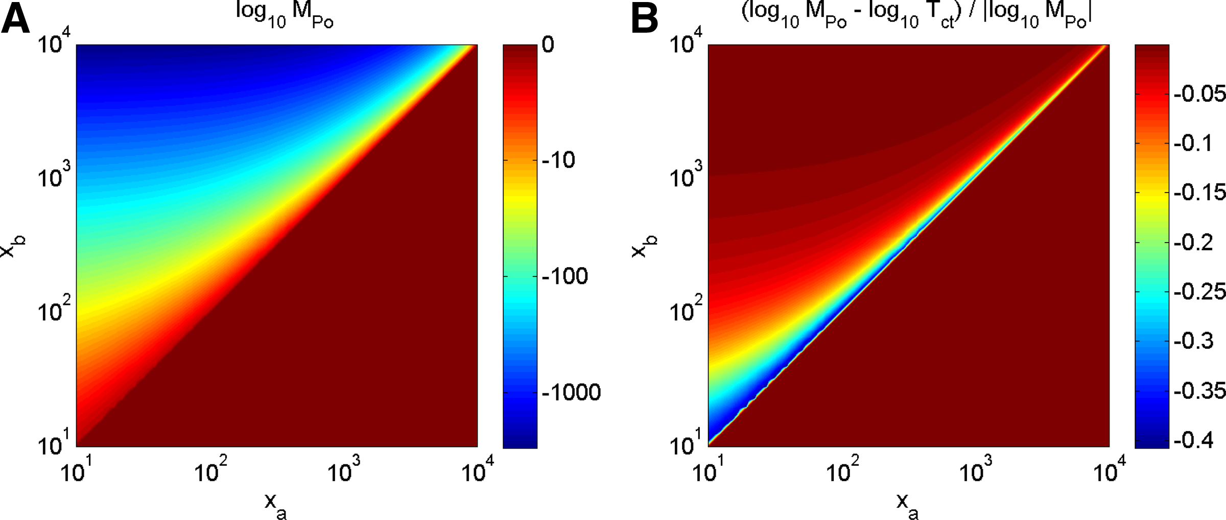
Figure 2A shows the numerical evaluation of \documentclass{aastex}\usepackage{amsbsy}\usepackage{amsfonts}\usepackage{amssymb}\usepackage{bm}\usepackage{mathrsfs}\usepackage{pifont}\usepackage{stmaryrd}\usepackage{textcomp}\usepackage{portland,xspace}\usepackage{amsmath,amsxtra}\pagestyle{empty}\DeclareMathSizes{10}{9}{7}{6}\begin{document}$${\cal M}_{Po}$$\end{document} across a range of counts that occur in practice. This figure clearly shows where the effects of the precision limits of IEEE-754 become apparent: the significant, dark blue shaded part of the plot corresponds to p-values < 10−400. The thousands of peaks in the experimental data discussed in Section 4 fall into this region (Kowalczyk et al., 2009). Note that the truncation of \documentclass{aastex}\usepackage{amsbsy}\usepackage{amsfonts}\usepackage{amssymb}\usepackage{bm}\usepackage{mathrsfs}\usepackage{pifont}\usepackage{stmaryrd}\usepackage{textcomp}\usepackage{portland,xspace}\usepackage{amsmath,amsxtra}\pagestyle{empty}\DeclareMathSizes{10}{9}{7}{6}\begin{document}$$\log_{10} {\cal M}_{Po}$$\end{document} at −500 is used in Figure 2A purely for the purpose of visualization.
3.2. Related statistical tests
The Poisson Margin test is closely related to some other statistical tests. This relationship has been explored elsewhere (Kowalczyk et al., 2009; Kowalczyk, 2009), and here we mention only the Counts test and the Coin Toss test.
For xa < xb, the Counts test is defined as
\documentclass{aastex}\usepackage{amsbsy}\usepackage{amsfonts}\usepackage{amssymb}\usepackage{bm}\usepackage{mathrsfs}\usepackage{pifont}\usepackage{stmaryrd}\usepackage{textcomp}\usepackage{portland,xspace}\usepackage{amsmath,amsxtra}\pagestyle{empty}\DeclareMathSizes{10}{9}{7}{6}\begin{document}\begin{align*}
T_* (x_a , x_b) : \ = \sup_{\mu_a \geq \mu_b > 0} {\mathbb P}
\left[X_a \leq x_a \ \& \ x_b < X_b \ \big| \ X_i \sim Poi (\mu_i)
\right] \tag{10}
\end{align*}\end{document}
and for xa < xb and the Coin Toss test as
\documentclass{aastex}\usepackage{amsbsy}\usepackage{amsfonts}\usepackage{amssymb}\usepackage{bm}\usepackage{mathrsfs}\usepackage{pifont}\usepackage{stmaryrd}\usepackage{textcomp}\usepackage{portland,xspace}\usepackage{amsmath,amsxtra}\pagestyle{empty}\DeclareMathSizes{10}{9}{7}{6}\begin{document}\begin{align*}
{\cal T}_{ct} (x_a , x_b) : \ = {\mathbb P} \left[X \leq x_a \
\Big | \ X \sim Bin \left(\frac {1} {2} , x_a + x_b \right)
\right] . \tag {11}
\end{align*}\end{document}
The Coin Toss test was used in Nix et al. (2008) and Rozowsky et al. (2009). The data from the latter article will be used for our experimental validation; hence, indirectly, we will be comparing against this statistic, and a clarification of its relationship to the Poisson Margin is appropriate here. Both articles have used Coin Toss for computing the statistical significance of the difference between two counts xa and xb in the same fashion as in the case of \documentclass{aastex}\usepackage{amsbsy}\usepackage{amsfonts}\usepackage{amssymb}\usepackage{bm}\usepackage{mathrsfs}\usepackage{pifont}\usepackage{stmaryrd}\usepackage{textcomp}\usepackage{portland,xspace}\usepackage{amsmath,amsxtra}\pagestyle{empty}\DeclareMathSizes{10}{9}{7}{6}\begin{document}$${\cal M}_{Po}$$\end{document}, but for the special case when libraries have equal, or equalized, sizes, namely |Ra| ≈ |Rb|. In this special case, they are “equivalent” to the \documentclass{aastex}\usepackage{amsbsy}\usepackage{amsfonts}\usepackage{amssymb}\usepackage{bm}\usepackage{mathrsfs}\usepackage{pifont}\usepackage{stmaryrd}\usepackage{textcomp}\usepackage{portland,xspace}\usepackage{amsmath,amsxtra}\pagestyle{empty}\DeclareMathSizes{10}{9}{7}{6}\begin{document}$${\cal M}_{Po}$$\end{document} test in the following sense.
Theorem 2
If |Ra| = |Rb| and the empirical proportion relation (3) holds, then\documentclass{aastex}\usepackage{amsbsy}\usepackage{amsfonts}\usepackage{amssymb}\usepackage{bm}\usepackage{mathrsfs}\usepackage{pifont}\usepackage{stmaryrd}\usepackage{textcomp}\usepackage{portland,xspace}\usepackage{amsmath,amsxtra}\pagestyle{empty}\DeclareMathSizes{10}{9}{7}{6}\begin{document}\begin{align*}
{\cal M}_{Po} (x_a , x_b) = T_* (x_a , x_b) \approx {\cal T}_{ct}
(x_a , x_b) .
\end{align*}\end{document}
Proof outline
If |Ra| = |Rb|, then λa < λb is equivalent to μa : = λa|Ra| < μb : = λb|Rb|; hence, the equivalence \documentclass{aastex}\usepackage{amsbsy}\usepackage{amsfonts}\usepackage{amssymb}\usepackage{bm}\usepackage{mathrsfs}\usepackage{pifont}\usepackage{stmaryrd}\usepackage{textcomp}\usepackage{portland,xspace}\usepackage{amsmath,amsxtra}\pagestyle{empty}\DeclareMathSizes{10}{9}{7}{6}\begin{document}$${\cal M}_{Po} (x_a , x_b) = T_* (x_a , x_b)$$\end{document} follows from the definitions (4) and (10). The approximation by \documentclass{aastex}\usepackage{amsbsy}\usepackage{amsfonts}\usepackage{amssymb}\usepackage{bm}\usepackage{mathrsfs}\usepackage{pifont}\usepackage{stmaryrd}\usepackage{textcomp}\usepackage{portland,xspace}\usepackage{amsmath,amsxtra}\pagestyle{empty}\DeclareMathSizes{10}{9}{7}{6}\begin{document}$${\cal T}_{ct}$$\end{document} has been argued in Kowalczyk (2009); here we demonstrate it by numerical evaluation presented in Figure 2.
Figure 2B shows a numerical evaluation of the differences between \documentclass{aastex}\usepackage{amsbsy}\usepackage{amsfonts}\usepackage{amssymb}\usepackage{bm}\usepackage{mathrsfs}\usepackage{pifont}\usepackage{stmaryrd}\usepackage{textcomp}\usepackage{portland,xspace}\usepackage{amsmath,amsxtra}\pagestyle{empty}\DeclareMathSizes{10}{9}{7}{6}\begin{document}$$\log_{10} {\cal M}_{Po} \big|_{\mid R_a \mid = \mid R_b \mid}$$\end{document} and \documentclass{aastex}\usepackage{amsbsy}\usepackage{amsfonts}\usepackage{amssymb}\usepackage{bm}\usepackage{mathrsfs}\usepackage{pifont}\usepackage{stmaryrd}\usepackage{textcomp}\usepackage{portland,xspace}\usepackage{amsmath,amsxtra}\pagestyle{empty}\DeclareMathSizes{10}{9}{7}{6}\begin{document}$$\log_{10} {\cal T}_{ct}$$\end{document} over a grid of values of xa and xb that occur in practice. Note the differences in the shading scales used in the two sub-figures. The difference \documentclass{aastex}\usepackage{amsbsy}\usepackage{amsfonts}\usepackage{amssymb}\usepackage{bm}\usepackage{mathrsfs}\usepackage{pifont}\usepackage{stmaryrd}\usepackage{textcomp}\usepackage{portland,xspace}\usepackage{amsmath,amsxtra}\pagestyle{empty}\DeclareMathSizes{10}{9}{7}{6}\begin{document}$$\mid \log_{10}{\cal M}_{Po} - \log_{10}{\cal T}_{ct} \mid$$\end{document} is < 2; hence, in the areas of significant values of \documentclass{aastex}\usepackage{amsbsy}\usepackage{amsfonts}\usepackage{amssymb}\usepackage{bm}\usepackage{mathrsfs}\usepackage{pifont}\usepackage{stmaryrd}\usepackage{textcomp}\usepackage{portland,xspace}\usepackage{amsmath,amsxtra}\pagestyle{empty}\DeclareMathSizes{10}{9}{7}{6}\begin{document}$$\log_{10} {\cal M}_{Po}$$\end{document}, say < −100, it composes practically negligible correction of ≤1%. This also allows the extension of the scaling properties \documentclass{aastex}\usepackage{amsbsy}\usepackage{amsfonts}\usepackage{amssymb}\usepackage{bm}\usepackage{mathrsfs}\usepackage{pifont}\usepackage{stmaryrd}\usepackage{textcomp}\usepackage{portland,xspace}\usepackage{amsmath,amsxtra}\pagestyle{empty}\DeclareMathSizes{10}{9}{7}{6}\begin{document}$${\cal T}_{ct}$$\end{document} discussed below to the case of \documentclass{aastex}\usepackage{amsbsy}\usepackage{amsfonts}\usepackage{amssymb}\usepackage{bm}\usepackage{mathrsfs}\usepackage{pifont}\usepackage{stmaryrd}\usepackage{textcomp}\usepackage{portland,xspace}\usepackage{amsmath,amsxtra}\pagestyle{empty}\DeclareMathSizes{10}{9}{7}{6}\begin{document}$${\cal M}_{Po} \big|_{\mid R_a \mid = \mid R_b \mid}$$\end{document}.
3.3. Scaling properties
The following result can be shown formally (Kowalczyk, 2009).
Theorem 3
(Scaling Power Law). Let 0 < 2xa < xb be two integers and κ > 1. Then\documentclass{aastex}\usepackage{amsbsy}\usepackage{amsfonts}\usepackage{amssymb}\usepackage{bm}\usepackage{mathrsfs}\usepackage{pifont}\usepackage{stmaryrd}\usepackage{textcomp}\usepackage{portland,xspace}\usepackage{amsmath,amsxtra}\pagestyle{empty}\DeclareMathSizes{10}{9}{7}{6}\begin{document}\begin{align*}
\log {\cal T}_{ct} (\kappa x_a , \kappa x_b) = \kappa \log {\cal
T}_{ct} (x_a , x_b) + \frac {o (x_b)} {x_b} , \tag {12}
\end{align*}\end{document}
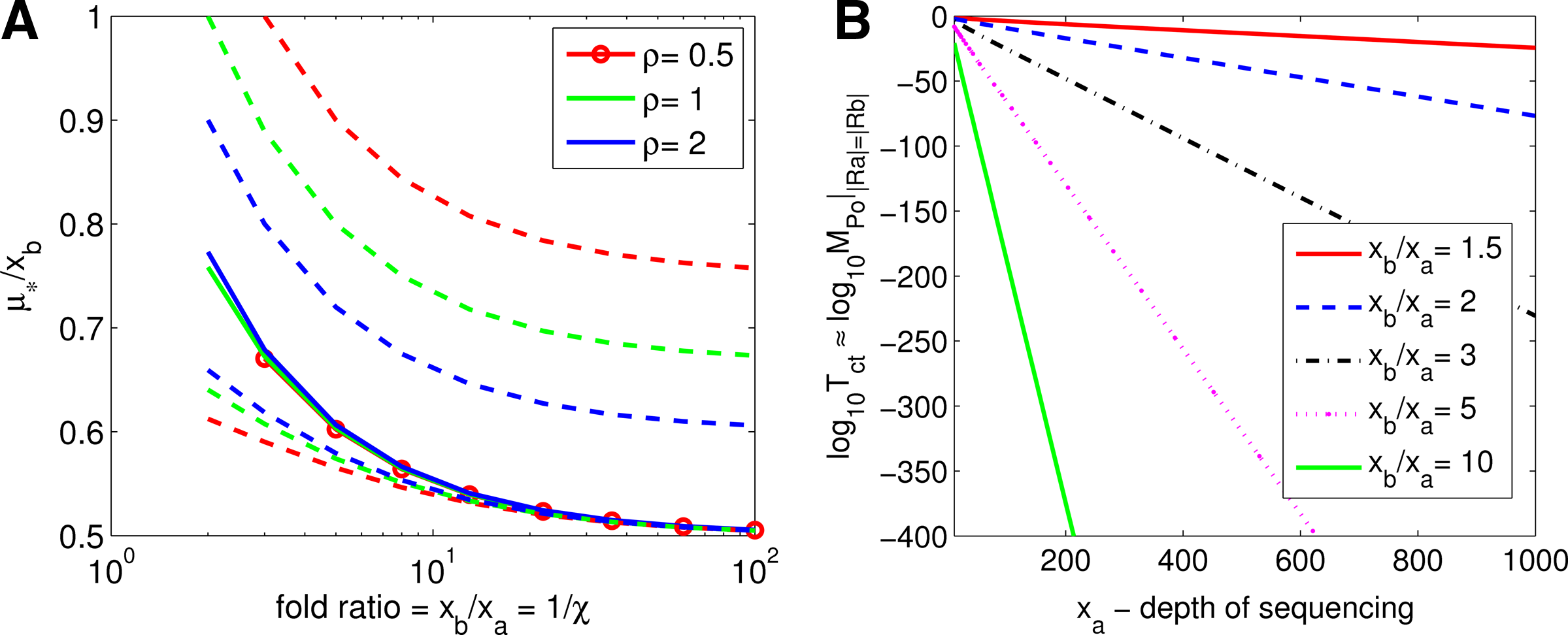
The computational validation of this result and implied practical extension to the whole range of values xb > 0 is presented in Figure 1B, which is sufficient for our discussion below. Plots there show clearly the asymptotical power scaling law (12): \documentclass{aastex}\usepackage{amsbsy}\usepackage{amsfonts}\usepackage{amssymb}\usepackage{bm}\usepackage{mathrsfs}\usepackage{pifont}\usepackage{stmaryrd}\usepackage{textcomp}\usepackage{portland,xspace}\usepackage{amsmath,amsxtra}\pagestyle{empty}\DeclareMathSizes{10}{9}{7}{6}\begin{document}$${\cal T}_{ct} (\kappa x_a , \kappa x_b) \approx {\cal T}_{ct} (x_a , x_b)^{\kappa}$$\end{document} translating to the linear dependence in the plots of the form \documentclass{aastex}\usepackage{amsbsy}\usepackage{amsfonts}\usepackage{amssymb}\usepackage{bm}\usepackage{mathrsfs}\usepackage{pifont}\usepackage{stmaryrd}\usepackage{textcomp}\usepackage{portland,xspace}\usepackage{amsmath,amsxtra}\pagestyle{empty}\DeclareMathSizes{10}{9}{7}{6}\begin{document}$$\log_{10} {\cal T}_{ct} (x_a , x_a / \chi) \approx x_a \times A^{- 1} \log_{10} {\cal T}_{ct} (A , A / \chi)$$\end{document}, where A ≫ 1 is a constant.
(A) Lower and upper bounds on μ* given by Eqn. (8) of Theorem 1 (broken lines) and compared to the exact values μ* given by solution of Eqn. 7; here we show averages for μ* as solid lines, the values for evaluation over xa-grid of 100 values logarithmically spaced between 1 and 1000 and corresponding xb : = xa/χ < 10,000. (B) Computational validation of the Scaling Power Law given by Theorem 3. The plots show clearly the asymptotical power scaling law (12): \documentclass{aastex}\usepackage{amsbsy}\usepackage{amsfonts}\usepackage{amssymb}\usepackage{bm}\usepackage{mathrsfs}\usepackage{pifont}\usepackage{stmaryrd}\usepackage{textcomp}\usepackage{portland,xspace}\usepackage{amsmath,amsxtra}\pagestyle{empty}\DeclareMathSizes{10}{9}{7}{6}\begin{document}$${\cal T}_{ct} (\kappa x_a , \kappa x_b) \approx {\cal T}_{ct} (x_a , x_b)^{\kappa}$$\end{document} translating to the linear dependence in the plots of the form \documentclass{aastex}\usepackage{amsbsy}\usepackage{amsfonts}\usepackage{amssymb}\usepackage{bm}\usepackage{mathrsfs}\usepackage{pifont}\usepackage{stmaryrd}\usepackage{textcomp}\usepackage{portland,xspace}\usepackage{amsmath,amsxtra}\pagestyle{empty}\DeclareMathSizes{10}{9}{7}{6}\begin{document}$$x_a \mapsto \log_{10} {\cal T}_{ct} (x_a , x_a / \chi) \approx x_a \times A^{- 1} \log_{10} {\cal T}_{ct} (A , A / \chi)$$\end{document}, where A ≫ 1 is a constant.
(A) Numerical evaluation of \documentclass{aastex}\usepackage{amsbsy}\usepackage{amsfonts}\usepackage{amssymb}\usepackage{bm}\usepackage{mathrsfs}\usepackage{pifont}\usepackage{stmaryrd}\usepackage{textcomp}\usepackage{portland,xspace}\usepackage{amsmath,amsxtra}\pagestyle{empty}\DeclareMathSizes{10}{9}{7}{6}\begin{document}$$\log_{10} {\cal M}_{Po} (x_a , x_b)$$\end{document} for the case of |Ra| = |Rb|. (B) Numerical evaluation of the relative difference \documentclass{aastex}\usepackage{amsbsy}\usepackage{amsfonts}\usepackage{amssymb}\usepackage{bm}\usepackage{mathrsfs}\usepackage{pifont}\usepackage{stmaryrd}\usepackage{textcomp}\usepackage{portland,xspace}\usepackage{amsmath,amsxtra}\pagestyle{empty}\DeclareMathSizes{10}{9}{7}{6}\begin{document}$$(\log_{10}$$\end{document}\documentclass{aastex}\usepackage{amsbsy}\usepackage{amsfonts}\usepackage{amssymb}\usepackage{bm}\usepackage{mathrsfs}\usepackage{pifont}\usepackage{stmaryrd}\usepackage{textcomp}\usepackage{portland,xspace}\usepackage{amsmath,amsxtra}\pagestyle{empty}\DeclareMathSizes{10}{9}{7}{6}\begin{document}$${\cal M}_{Po} -\log_{10}{\cal T}_{ct}) / \log_{10}{\cal M}_{Po}$$\end{document}. The evaluation has been done for the regular logarithmic grid of count values 1 ≤ xa, xb ≤ 10,000.
The above Theorem and Figure 1B facilitate a discussion of two important issues in the analysis of the NGS data, namely, (i) the impact of the number of lanes use by the sequencing machine to map the library and (ii) scaling of the counts, in the case of typically unequal sizes of the sequenced and then mapped tag sets. First, they tell us that having κ times more reads sequenced, for example, using κ lanes in the sequencing machine rather than one, will provide exponentially stronger (i.e., smaller, exponentiated by κ) p-values, asymptotically for large xb. This can be used, for example, as guidance for selection of more or fewer lanes in an NGS experiment.
However, those results also point to fragility of “count scaling.” More precisely, if the numbers of reads actually sequenced and mapped are significantly different, |Ra| ≠ |Rb|, then either we need statistical tests that are intrinsically immune to such differences, or we need to normalize the counts in a candidate peak region to make them comparable. The \documentclass{aastex}\usepackage{amsbsy}\usepackage{amsfonts}\usepackage{amssymb}\usepackage{bm}\usepackage{mathrsfs}\usepackage{pifont}\usepackage{stmaryrd}\usepackage{textcomp}\usepackage{portland,xspace}\usepackage{amsmath,amsxtra}\pagestyle{empty}\DeclareMathSizes{10}{9}{7}{6}\begin{document}$${\cal M}_{Po}$$\end{document} test (4) falls in the first category, whereas the \documentclass{aastex}\usepackage{amsbsy}\usepackage{amsfonts}\usepackage{amssymb}\usepackage{bm}\usepackage{mathrsfs}\usepackage{pifont}\usepackage{stmaryrd}\usepackage{textcomp}\usepackage{portland,xspace}\usepackage{amsmath,amsxtra}\pagestyle{empty}\DeclareMathSizes{10}{9}{7}{6}\begin{document}$${\cal T}_{ct}$$\end{document} test represents the latter.
4. Experimental Validation
It is far from clear that the postulated statistical test will provide useful results in practice. Simply put, the worst case scenario embraced in definition (4) may be too conservative and the generated p-values too close to 1 to be informative. In order to address this concern, we have decided to focus on the well-studied NGS application of ChIP-Seq peak calling, which involves comparison of only two libraries (the target and the dedicated control). The more complex problem of differential analysis of multiple libraries will be addressed in future work.
In order to validate our method, we have used public domain ChIP-Seq data. In particular, Rozowsky et al. (2009) provides 36,998 putative locations/regions for binding STAT1 and 24,739 locations/regions for Pol II. Note that both databases in Rozowsky et al. (2009) have been used as the basis of the most recent ENCODE data in their correponding domains; hence, we have no alternative “gold standards” to evaluate the results of our analysis. In this article, we deal with this obstacle by using a procedure evaluating the results of analysis by checking their internal consistency. This procedure is outlined below in Section 4.3.
Since Rozowsky et al. (2009) also provides the Eland mappings of the tags for the controls, and STAT1 and Pol II data sets, we have performed an additional independent analysis of this data using Poisson Margin outlined in the following two sections.
4.1. Re-ordering
We have used the list of peak ranges, peak locations, and range boundaries exactly as in Rozowsky et al. (2009). For each range, we have extracted (raw) counts, following the protocol described in the original article, and then we used the \documentclass{aastex}\usepackage{amsbsy}\usepackage{amsfonts}\usepackage{amssymb}\usepackage{bm}\usepackage{mathrsfs}\usepackage{pifont}\usepackage{stmaryrd}\usepackage{textcomp}\usepackage{portland,xspace}\usepackage{amsmath,amsxtra}\pagestyle{empty}\DeclareMathSizes{10}{9}{7}{6}\begin{document}$${\cal M}_{Po}$$\end{document} statistic to allocate the p-value (see Table 1 for STAT1 and Table 2 for Pol II in Supplementary material in Kowalczyk et al. [2009]). Although the order according to the \documentclass{aastex}\usepackage{amsbsy}\usepackage{amsfonts}\usepackage{amssymb}\usepackage{bm}\usepackage{mathrsfs}\usepackage{pifont}\usepackage{stmaryrd}\usepackage{textcomp}\usepackage{portland,xspace}\usepackage{amsmath,amsxtra}\pagestyle{empty}\DeclareMathSizes{10}{9}{7}{6}\begin{document}$${\cal M}_{Po}$$\end{document} method is only slightly different from the original, the overlap is >90% (Table 1); the differences in performance benchmarks especially for STAT1 are significant.
Summary of Ordered Peaks Lists Overlap with the List in Rozowsky et al. (2009) and the Accuracy Prediction of Binding Site on the Whole Genome
In experiments I–IV, we use data on chromosome 22 for training SVM exclusively. All values listed are in %.
Boldface marks the most significant results within each group of experiments, I–II and III–IV, respectively.
4.2. De novo significant range location
In our experiments described below, we have implemented and run a fixed size sliding window method across the genome comparing the number of tags in each window for the control and target samples, for each sample for both DNA strands pooled together. Regions of significance are then defined by thresholding the p-values obtained from the Poisson Margin test. This resembles the approach in Zhang et al. (2008). This effectively separates the tasks of finding regions of the genome where we believe a peak lies and determining the location of the antibody binding site itself—the former task being done efficiently on the whole genome scale and the latter being done intensively on just those regions identified by the genome wide scan as containing a peak. The genome was scanned sequentially with a window of 200 bp, shifted every four bases, which took about 17 minutes on a workstation with 2GHz Opteron CPUs and 32Gb of main memory.
We have identified 35,229 peak ranges for STAT1 using un-adjusted p-values < 1E-4 and 28,890 using un-adjusted p-values < 1E-6 for Pol II, with thresholds chosen to match the numbers of peaks in the original publication. The range was defined as a contiguous region of 200 BP blocks that passed the threshold.
Such a procedure can be followed by refinements of boundaries, more precise location of the range boundaries, and more precise peak location. Example of such secondary adjustments can be found elsewhere (Rozowsky et al., 2009; Zhang et al., 2008; Ji et al., 2008), but we used none here.
4.3. Genome annotation test
We wish to quantify consistency of the putative peak ranges by quantifying ability to predict those locations on the whole genome by a predictor trained on a part of the genome. In our experiments, peak ranges from chromosome 22 were used for training, and those from the remaining chromosomes were used only for testing. For quantifying prediction accuracy, we have adapted protocol 1B in the literature (Sonnenburg et al., 2006; Abeel et al., 2009; Bedo et al., 2009). In brief, the genome is divided into 500bp non-overleaping segments (total of 5,362,342 segments not containing ‘N's), with each segment labeled as positive if it overlaps a peak range and negative otherwise (the positive segments comprise <1% of the total number of segments). These labels were used to build a predictor and verify its performance measured by precision and recall. We recall that “Precision” means ratio of true positive retrieved (for a given decision threshold) to number of retrieved cases, and “Recall” is the number of true positive retrieved divided by the total number of true positive cases.
A linear support vector machine (SVM) was developed to label each 500bp segment independently (Bedo et al., 2009). Each 500bp segment was represented as a feature vector containing frequency counts of 4-mers contained within. Recursive feature elimination was used to reduce the model's number of features, and other meta-parameters were set to maximize the area under precision-recall curve (PRC) in an internal cross-validation on the training data.
This method works very well for some tasks such as the prediction of transcription start sites and the binding of some transcription factors (e.g., c-Myc) (Bedo et al., 2009) and seems to significantly outperform other methods such as standard position weight matrices (PWM). From our experience, STAT1 is one of the harder transcription factors to predict; however, we still observe much higher performance using the SVM predictor than with PWMs (Bedo et al., 2009).
4.4. Results
Table 1 and Figure 3 summarize results for a few variations of genome annotation experiments described above, for STAT1 and Pol II data, respectively. As we recall, the data from chromosome 22 were used for training exclusively, and test results reported are for data from the whole genome. The following four basic variations of the experiment consisted in usage of different sets of peaks:
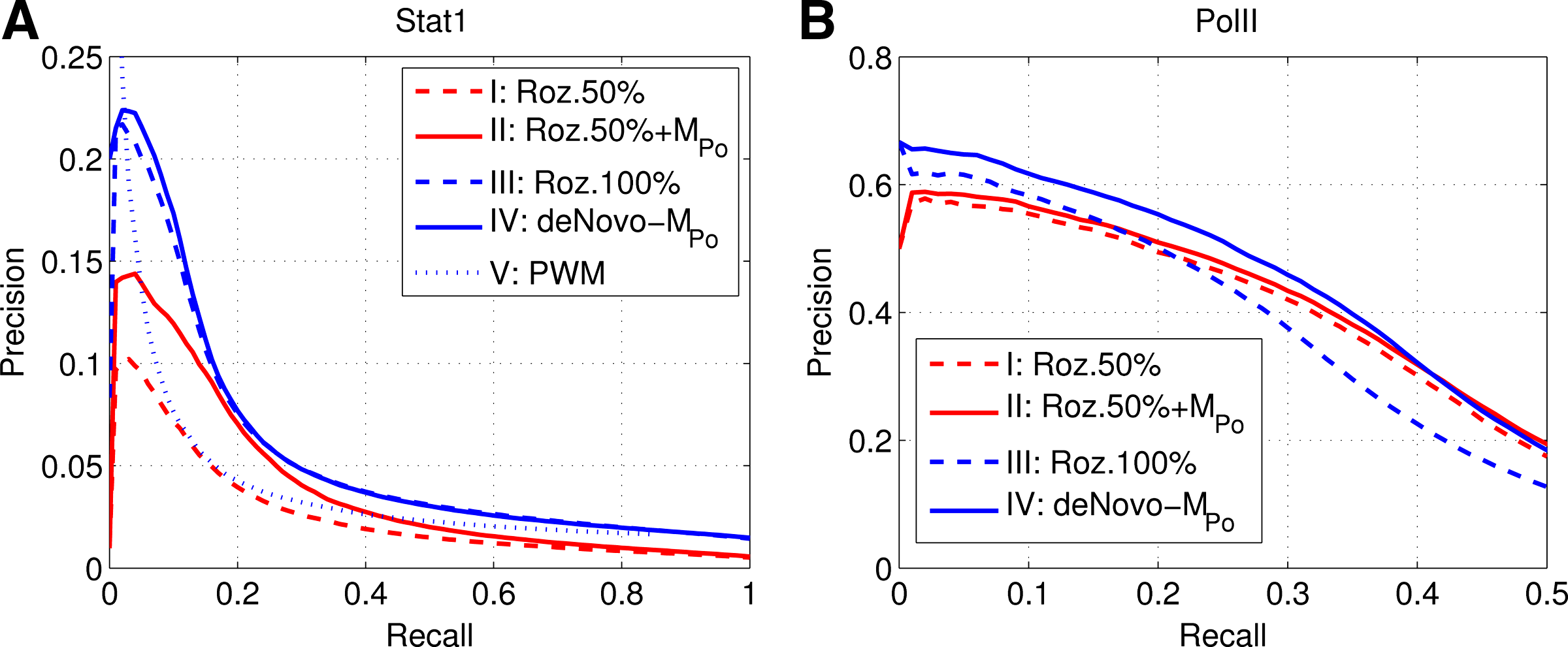
I: The top 50% of the original list in Rozowsky et al. (2009)
II: The top 50% of the list in Rozowsky et al. (2009) after sorting by \documentclass{aastex}\usepackage{amsbsy}\usepackage{amsfonts}\usepackage{amssymb}\usepackage{bm}\usepackage{mathrsfs}\usepackage{pifont}\usepackage{stmaryrd}\usepackage{textcomp}\usepackage{portland,xspace}\usepackage{amsmath,amsxtra}\pagestyle{empty}\DeclareMathSizes{10}{9}{7}{6}\begin{document}$${\cal M}_{Po}$$\end{document} method
III: The whole 100% list in Rozowsky et al. (2009)
IV: A de novo list of peaks derived as outlined in Section 4.2
Precision–recall curves for STAT1 (A) and Pol II (B) corresponding to Table 1. We report test results for the whole genome for the variants I–V of the genome annotation test experiment described in Section 4.4.
Additionally, for STAT1 we have also tested a typical PWM from TRANSFAC® 7.0. This is reported as row “V” in Table 1. In this case, the “score” per range in Rozowsky et al. (2009) is defined as the max of PWM scores for all positions within a 500BP tile. The overlap in Table 1 was calculated using the top 37k tiles as scored by the PWM.
We observe that, for variants I and II for STAT1, the area under the PRC curve (4.0%) is approximately 1.5 times that for the original Rozowsky et al. (2009) ordering (2.6%). For Pol II, the corresponding difference is smaller, due to larger similarity of the ordered lists and much higher accuracy of predictions, but differences between de-novo (blue solid) and 100% list (broken blue) in Rozowsky et al. (2009) in Figure 3B is well pronounced.
5. Discussion
The basic protocol described in this article can be extended in a number of directions. In the experiments, we have used only uniquely mapped reads. The density of such reads varies along the genome, which can affect the relative p-values for peaks at different locations since both \documentclass{aastex}\usepackage{amsbsy}\usepackage{amsfonts}\usepackage{amssymb}\usepackage{bm}\usepackage{mathrsfs}\usepackage{pifont}\usepackage{stmaryrd}\usepackage{textcomp}\usepackage{portland,xspace}\usepackage{amsmath,amsxtra}\pagestyle{empty}\DeclareMathSizes{10}{9}{7}{6}\begin{document}$${\cal M}_{Po}$$\end{document} and the Coin Tossing statistic (\documentclass{aastex}\usepackage{amsbsy}\usepackage{amsfonts}\usepackage{amssymb}\usepackage{bm}\usepackage{mathrsfs}\usepackage{pifont}\usepackage{stmaryrd}\usepackage{textcomp}\usepackage{portland,xspace}\usepackage{amsmath,amsxtra}\pagestyle{empty}\DeclareMathSizes{10}{9}{7}{6}\begin{document}$${\cal T}_{ct}$$\end{document}) (Rozowsky et al., 2009) are sensitive to the sequencing depth (Fig. 1B). A simple way around this obstacle is to scale up the observed counts (per range) inversely to the fraction of mappable tags for the region. Such information for uniquely mapped tags of length 30 is provided in Rozowsky et al. (2009), but information of uniquely mapped up to two mismatches (which we prefer) is not currently available (Rozowsky et al., 2009). We have not used this correction here.
We present an alternative to the methods introduced previously (Rozowsky et al., 2009; Robertson et al., 2007; Zhang et al., 2008) (and see Pepke et al. [2009] for a recent review of these and other ChIP-seq computational methods). We have focused on the first of those references, since it is one of the most recent and allows access to good quality of experimental data, included in ENCODE. We have shown that a principled analysis of such data using our method is feasible with minimal need for (arbitrary) design choices and with a minimal number of data-adjustable parameters. (An illustrating example here is the introduction in Rozowsky et al. [2009] of an ad hoc parameter 0 ≤ Pf ≤ 1 for the fraction of putative highest peaks to be excluded from regression for local normalization of counts.) Our approach is robust, and can be applied to a wide variety of experimental designs involving different numbers of samples, possibly from different cell lineages. It is applicable precisely because it does not require scaling of the individual libraries of reads. The results in Kowalczyk (2009) and Section 3.3 show that such a scaling, if applied, should be done with extreme caution, if the analysis is to be meaningful.
6. Conclusion
We have developed a principled statistical test for the detection of significant read concentrations that is directly applicable to libraries of different (unmatched) sizes without any scaling of read counts and have demonstrated that such a scaling could introduce significant bias in the computed p-values. Although our statistical test targets differential analysis for multiple NGS libraries, the initial validation in this article is restricted to the simplest case of comparison of a target library to a matching reference. Using the recent Encode Chip-Seq data, we have shown that our test delivers non-vacuous results, with peak calling accuracies comparable or even improved with respect to the original dedicated algorithm. The absence of adequate gold standards for benchmarking was circumvented by application of a novel internal consistency check based on the accuracy of generalization of a supervised learning predictor. Demonstration of the utility of that protocol is the second major contribution of this article.
Footnotes
Acknowledgments
NICTA is funded by the Australian Government's Department of Communications, Information Technology and the Arts, the Australian Research Council through Backing Australia's Ability, and the ICT Centre of Excellence programs.
Disclosure Statement
No competing financial interests exist.
References
1.
AbeelT., Van de PeerY., SaeysY.2009. Toward a gold standard for promoter prediction evaluation. Bioinformatics, 25:i313–i320.
2.
BaggerlyK.A., DengL., MorrisJ.S.et al.2003. Differential expression in SAGE: accounting for normal between-library variation. Bioinformatics, 19:1477–1483.
3.
BedoJ., MacIntyreG., HavivI.et al.2009. Simple SVM based whole-genome segmentation. http://dx.doi.org/10.1038/npre.2009.3811.1. 2010 December 1.
4.
Bloushtain-QimronN., YaoJ., SnyderE.2008. Cell type-specific DNA methylation patterns in the human breast. Proc. Natl. Acad. Sci. USA, 105:14076–14081.
5.
JiH., JiangH., MaW.et al.2008. An integrated software system for analyzing ChIP-chip and ChIP-seq data. Nat. Biotechnol., 26:1293–1300.
6.
KeepingE.1995. Introduction to Statistical InfernceReprint of 1962 edition byD. Van Nostrand Co.: Dover, New York.
KowalczykA., BedoJ., ConwayT.et al.2009. Poisson margin test for normalisation free significance analysis of NGS data [Supplementary Materials]http://www.genomics.csse.unimelb.edu.au/peakfiltsup. 2010 December 1.
9.
NixD., CourdyS., BoucherK.2008. Empirical methods for controlling false positives and estimating confidence in ChIP-seq peaks. BMC Bioinformatics, 9:523.
10.
PepkeS., WoldB., MortazaviA.2009. Computation for ChIP-seq and RNA-seq studies. Nat. Methods, 6:S22–S32.
11.
RobertsonG., HirstM., BainbridgeM.et al.2007. Genome-wide profiles of STAT1 DNA association using chromatin immunoprecipitation and massively parallel sequencing. Nat. Methods, 4:651–657.
12.
RobinsonM., SmythG.2007. Moderated statistical tests for assessing differences in tag abundance. Bioinformatics, 23:2881–2887.
13.
RozowskyJ., EuskirchenG., AuerbachR.et al.2009. Peakseq enables systematic scoring of chip-seq experiments relative to controls. Nat. Biotechnol., 27:66–75.
14.
SonnenburgS., ZienA., RatschG.2006. Arts: accurate recognition of transcription starts in human. Bioinformatics, 22:e423–e480.
15.
ZangC., SchonesD.E., ZengC.et al.2009. A clustering approach for identification of enriched domains from histone modification ChIP-Seq data. Bioinformatics, 25:1952–1958.