Computing a Consensus Phylogeny via Leaf Removal

Abstract

Given a set $T = {T_{1}, T_{2}, \dots, T_{m}}$ . of phylogenetic trees with the same leaf-label set X, we wish to remove some leaves from the trees so that there is a tree T with leaf-label set X displaying all the resulting trees. Note that the labels of leaves removed from one input tree may be different from those of leaves removed from another input tree. One objective is to minimize the total number of leaves removed from the trees, whereas the other is to minimize the maximum number of leaves removed from an input tree. Chauve et al. refer to the problem with the first (respectively, second) objective as AST-LR (respectively, AST-LR-d), and they show that both problems are NP-hard, where NP is the class of problems solvable in non-deterministic polynomial time. They further present algorithms for the parameterized versions of both problems. In this article, we point out that their algorithm for the parameterized version of AST-LR is flawed and present a new algorithm. Since neither Chauve et al.'s algorithm for AST-LR-d nor our new algorithm for AST-LR looks practical, we further design integer-linear programming (ILP for short) models for AST-LR and AST-LR-d, and we discuss speedup issues when using popular ILP solvers (say, GUROBI or CPLEX) to solve the models. Our experimental results show that our ILP approach is quite efficient.

1. Introduction

When studying the evolutionary history of a set X of existing species, one can obtain a phylogenetic tree with leaf set X with high confidence by looking at a segment of sequences or a set of genes (Ma et al., 1999; Ma and Zhang, 2011). When looking at different segments of sequences, different phylogenetic trees with leaf set X can be obtained with high confidence, too. To facilitate the comparison of the resulting trees, a number of distance metrics have been proposed in the literature (Buneman, 1971; Robinson and Foulds, 1981; Li et al., 1996; Swofford et al., 1996; Chauve et al., 2017). Among the metrics, the rSPR-distance (Bordewich and Semple, 2005) is an important metric that often helps us discover reticulation events. In particular, it provides a lower bound on the number of reticulation events (Beiko and Hamilton, 2006; Baroni et al., 2015), and it has been regularly used to model reticulate evolution (Maddison, 1997; Nakhleh et al., 2005).

The rSPR distance is usually defined for two phylogenetic trees, T₁ and T₂. It can be defined as the minimum number of edges that should be deleted from each of T₁ and T₂ to transform them into topologically identical rooted forests F₁ and F₂. Roughly speaking, F₁ and F₂ are topologically identical if they become identical forests after repeatedly contracting an edge (p, c) in each of them such that c is the unique child of p (until no such edge exists). The problem of computing the rSPR distance of two trees is NP-hard (Hein et al., 1996; Bordewich and Semple, 2005). This has motivated researchers to design approximation algorithms for the problem (Schalekamp et al., 2016; Chen et al., 2017) as well as fixed-parameter algorithms for the problem (Whidden et al., 2010; Chen et al., 2015, 2017).

Recently, Chauve et al. (2017) defined two new metrics highly related to the rSPR distance. Basically, to compute the rSPR distance of two phylogenetic trees, we are allowed to delete any edges from the input trees so that the resulting forests become topologically identical, as long as the number of deleted edges is minimized. In contrast, the two new metrics defined by Chauve et al. (2017) require that any edge removed from the input trees must be incident to a leaf. Moreover, the new metrics are defined for any number of phylogenetic trees and also allow that the labels of leaves removed from one input tree are different from those of leaves removed from another input tree. More specifically, given a set of phylogenetic trees, the two new metrics ask us to remove leaves from the input trees so that there is a single tree displaying all the resulting trees, where a tree T displays another tree T′ if and only if T′ is topologically identical to a subtree of T. One of the metrics requires that the total number of leaves removed from the input trees is minimized, whereas the other requires that the maximum number of leaves removed from an input trees is minimized. The problem of computing the former metric is denoted by AST-LR, whereas the latter is denoted by AST-LR-d. Here, AST stands for “agreement subtree” and LR stands for “leaf removal.”

A problem related to AST-LR is the maximum agreement supertree problem (MASP) defined in Jansson et al. (2005). Given a set {T₁, …, T_m} of phylogenetic trees not necessarily with the same leaf-label set, MASP asks to compute a maximum set L of leaf-labels in the input trees so that there is a phylogenetic tree with leaf-label set L displaying the trees T₁|_L, …, T_m|_L, where for each i∈{1, …, m}, T_i|_L denotes the phylogenetic tree obtained from T_i by deleting those leaves whose labels are not in L. Jansson et al. (2005) show the NP-hardness of MASP and present polynomial-time algorithms for several special cases.

As easily observed in Chauve et al. (2017), the special cases of AST-LR and AST-LR-d where there are only two input trees are basically the maximum agreement subtree problem and hence can be solved in $O (n log n)$ time (Cole et al., 2000). However, Chauve et al. (2017) show that both AST-LR and AST-LR-d are NP-hard in general. They then present an algorithm for the parameterized version of each of the problem. Their algorithm for the parameterized version of AST-LR (respectively, AST-LR-d) runs in $O (12^{q} m n^{3})$ [respectively, $O (288^{d} d^{3 d} (n^{2} + m n log n))$ ] time, where m is the number of input trees, n is the number of leaves in each input tree, and q (respectively, d) is the parameter.

In this article, we point out that the algorithm in Chauve et al. (2017) for the parameterized version of AST-LR is flawed and we present a new algorithm. The algorithm runs in $O ({(4 q - 2)}^{q} m^{2} n^{2})$ time. The idea behind our algorithm is as follows. First, it uses Aho et al.'s polynomial-time algorithm (Aho et al., 1981) for a related problem to find a set of pendant subtrees in the input trees. It then uses the subtrees to find a set S of at most 4q − 2 leaves in the input trees such that at least one leaf in S has to be deleted to have a required solution. It is worth pointing out that our algorithm actually solves a more general problem (than the parameterized version of AST-LR), where we allow the input trees to have different leaf-label sets.

Unfortunately, neither Chauve et al.'s algorithm for AST-LR-d nor our new algorithm for AST-LR looks practical. So, we further design integer-linear programming (ILP for short) models for AST-LR and AST-LR-d, and we discuss speedup issues when using popular ILP solvers (say, GUROBI or CPLEX) to solve the models. To evaluate the performance of our ILP models, we implement the algorithm in Chauve et al. (2017) for a much simpler parameterized problem (than the parameterized version of AST-LR), where we are only required to decide whether we can delete a total number of at most q leaves from the input trees so that the resulting trees have no conflicting triplets. Our experimental results show that GUROBI can solve our ILP model for AST-LR within a much shorter time than Chauve et al.'s algorithm solves this much simpler parameterized problem.

The remainder of this article is organized as follows. Section 2 gives the basic definitions that will be used thereafter. Section 3 is devoted to the parameterized version of AST-LR. Section 4 presents our ILP models for AST-LR and AST-LR-d and evaluates their efficiency experimentally.

2. Preliminaries

Throughout this article, a phylogenetic tree always means a rooted tree whose leaves are distinctly labeled. Unless stated otherwise, a phylogenetic tree is always binary, that is, each nonleaf vertex has exactly two children in the tree.

Let T be a phylogenetic tree. For each vertex v of T, the subtree rooted at v is called a pendant subtree of T. We use X(T) to denote the leaf-label set of T. For each x∈X(T), we use x^T to denote the leaf of T labeled x. Moreover, for a subset Y of X(T), we use Y^T to denote {x^T | x∈Y}. If T is clear from the context, we simply write x and Y instead of x^T and Y ^T, respectively. Moreover, for a subset Y of X(T), we use T − Y to denote the phylogenetic tree obtained from T by first removing the leaves in Y^T and further repeatedly removing an unlabeled leaf or contracting an edge, leaving a unifurcate vertex (i.e., vertex with only one child) until no such leaf or edge exists. We use T|_Y to denote T − (X(T)\Y). T displays another phylogenetic tree T′ if X(T′) ⊆ X(T) and T′ = T|_X(T′₎.

A leaf-prune-and-regraft (LPR) operation on T is the operation of replacing T by another phylogenetic tree T′ with X(T) = X(T′) such that T and T′ are different but T − {x} and T′ − {x} are identical, In other words, T′ is obtained from T as follows.

Choose a leaf x and an edge e = (u, v) of T such that v is neither the sibling nor the parent of x in T.

Remove the edge entering x and contract the edge leaving p, where p was the parent of x before the removal.

Replace e by three edges (u, w), (w, v), and (w, x), where w is a new vertex.

We say that T′ is obtained from T by pruning x and regrafting it on e. Intuitively speaking, LPR operations are rSPR operations [defined in Bordewich and Semple (2005)] restricted to leaves.

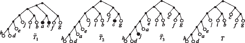
Let (T₁, …, T_m) be a list of phylogenetic trees, where it is unnecessary that X(T₁)…=X(T_m). A leaf-disagreement for (T₁, …, T_m) is a list L=(Y₁, …, Y_m) such that each Y_i (1 ≤i ≤ m) is a set of leaves in T_i and there is a phylogenetic tree T displaying T₁ - Y₁ through T_m − Y_m. The size of L is $\sum_{i = 1}^{m} | Y_{i} |$ , the radius of L is ${max}_{i = 1}^{m} | Y_{i} |$ , and T is called a center tree witnessing L. For example, consider the three trees $\tilde{T}$ ₁, $\tilde{T}$ ₂, and $\tilde{T}$ ₃ in Figure 1; if each Y_i (1 ≤ i ≤ 3) consists of the black leaves in $\tilde{T}$ _i,, then (Y₁, Y₂, Y₃) is a leaf-disagreement of size 4 and radius 2 for ( $\tilde{T}$ ₁, $\tilde{T}$ ₂, $\tilde{T}$ ₃) because the tree T in the figure displays all of $\tilde{T}$ ₁ − Y₁, $\tilde{T}$ ₂ − Y₂, and $\tilde{T}$ ₃ − Y₃. For an integer k, a size-k (respectively, radius-k) center tree for {T₁, …, T_m} is a center tree witnessing a leaf-disagreement of size (respectively, radius) at most k for (T₁, …, T_m). T₁, …, T_m are compatible if (θ, …, θ) is a leaf-disagreement for (T₁, …, T_m).

FIG. 1.

A counterexample to the algorithm for AST-LR in Chauve et al. (2017).

Given a set {T₁, …, T_m} of phylogenetic trees with $X (T_{1}) = \dots = X (T_{m})$ , the AST-LR (respectively, AST-LR-d) problem asks for the computation of a leaf-disagreement for (T₁, …, T_m) whose size (respectively, radius) is minimized over all leaf-disagreements for (T₁, …, T_m).

Let T₁ and T₂ be two phylogenetic trees with X(T₁) = X(T₂). A leaf-disagreement (Y₁, Y₂) for (T₁, T₂) is one-sided if Y₂ =θ. As easily observed in Chauve et al. (2017), the following hold:

For every leaf-disagreement (Y₁, Y₂) for (T₁, T₂), (Y₁ ∪ Y₂, θ) is a one-sided leaf-disagreement for (T₁, T₂).

For every one-sided leaf-disagreement (Y, θ) for (T₁, T₂) and for every Y₁ ⊆ Y, (Y₁, Y\Y₁) is a leaf-disagreement for (T₁, T₂).

For simplicity, we use Y to denote a one-sided leaf-disagreement (Y, θ) for (T₁, T₂). Y is minimal if for every y∈Y, and Y \ {y} is not a one-sided leaf-disagreement for (T₁, T₂). We use d_LR(T₁, T₂) to denote the minimum size of a one-sided leaf-disagreement Y for (T₁, T₂). Given T₁ and T₂, d_LR(T₁, T₂) can be computed in $O (n log n)$ time, where n = |X(T₁)| (Cole et al., 2000). Moreover, by the observation just made, d_LR(T₁, T₂) (respectively, $⌈\frac{1}{2} d_{L R} (T_{1}, T_{2})⌉$ ) is the minimum size (respectively, radius) of a leaf-disagreement for (T₁, T₂). In other words, if we require that there are only two trees in the input, then the AST-LR and the AST-LR-d problems become basically the same problem and can be solved in $O (n log n)$ time.

3. Parameterized Algorithm For AST-LR

A triplet is a phylogenetic tree with exactly three leaves. We use xy|z to denote the triplet t such that X(t) = {x, y, z} and x and y are siblings in t. Two triplets t₁ and t₂ conflict if t₁ = xy|z and t₂∈{xz|y, yz|x}. We say that xy|z is a triplet of a phylogenetic tree T if {x, y, z} ⊆ X(T) and T|_{{x, y, z}} = xy|z. For example, in Figure 1, ac|b is a triplet of $\tilde{T}$ ₁ whereas ab|c is a triplet of $\tilde{T}$ ₂ and $\tilde{T}$ ₃. For a phylogenetic tree T, we use tr(T) to denote the set of triplets in T. Moreover, for a set $T$ of phylogenetic trees, we use $t r (T)$ to denote $⋃_{T \in T} t r (T)$ , and we use $X (T)$ to denote $⋃_{T \in T} X (T)$ . A triple {x, y, z} is inconsistent in $T$ if $t r (T)$ has two conflicting triplets with label set {x, y, z}. For example, if $T$ consists of $\tilde{T}$ ₁, $\tilde{T}$ ₂, and $\tilde{T}$ ₃ in Figure 1, then the triple {a, b, c} is inconsistent in $T$ . A full set of triplets on a set $X$ of labels is a set $S$ of triplets such that $X = X (S)$ and $S$ contains exactly one of xy|z, xz|y, and yz|x for each triple ${x, y, z} \subseteq X$ .

3.1. The flaw in Chauve et al.'s algorithm

We first review Chauve et al.'s algorithm for the parameterized version of AST-LR. An instance of the parameterized version consists of an integer q and a set {T₁, …, T_m} of phylogenetic trees with X(T₁) = ⋯ = X(T_m), and the objective is to decide whether there is a leaf-disagreement L of size at most q for (T₁, …, T_m). Chauve et al.'s algorithm for the problem actually solves a more general problem. More specifically, the condition X(T₁) = ⋯ = X(T_m) on {T₁, …, T_m} is removed. Moreover, in addition to q and {T₁, …, T_m}, the input to their algorithm also includes a set F of non-conflicting triplets and the algorithm is supposed to return “yes” if and only if there is a leaf-disagreement L of size at most q for (T₁, …, T_m) such that some center tree T witnessing L satisfies that every triplet in F is a triplet of T. The triplets in F are called the fixed triplets. A triplet t∈F conflicts with a tree T_i if T_i has a triplet conflicting with t.

Obviously, to solve the parameterized version for (q, {T₁, …, T_m}), it suffices to solve the generalized problem for (q, {T₁, …, T_m}, θ). So, consider the call of Chauve et al.'s algorithm on input $(q, {T_{1}, \dots, T_{m}}, \emptyset)$ with X(T₁) = ⋯ = X(T_m). Since the algorithm is recursive, we need to consider a call originated from the root call [i.e., the call on input (q, {T₁, …, T_m}, θ)] after zero or more subsequent calls. Let ( $\tilde{q}$ , { $\tilde{T}$ ₁, …, $\tilde{T}$ _m}, $\tilde{F}$ ) be the input to the call. In the base case where $\tilde{q}$ < 0 or $\tilde{F}$ contains conflicting triplets, the algorithm returns “no.” Otherwise, it proceeds in two phases. In the first phase, it tries to find either a triplet t ∈ $\tilde{F}$ conflicting with some $\tilde{T}$ _i (1 ≤ i ≤ m) or a triple S inconsistent in { $\tilde{T}$ ₁, …, $\tilde{T}$ _m}. The first phase ends if neither t nor S is found. So, suppose that t or S is found.

Case 1: A triplet t = xy|z∈ $\tilde{F}$ conflicting with some $\tilde{T}$ _i (1 ≤ i ≤ m) is found. In this case, xz|y or yz|x is a triplet in $\tilde{T}$ _i. So, for each u∈{x, y, z}, the algorithm makes a recursive call on input $(\tilde{q} - 1, {{\tilde{T}}_{1}, \dots, {\tilde{T}}_{i - 1}, {\tilde{T}}_{i} - {u}, {\tilde{T}}_{i + 1}, \dots, {\tilde{T}}_{m}}, \tilde{F})$ . The algorithm returns “yes” if and only if at least one of the three recursive calls returns “yes.”

Case 2: A triple S = {x, y, z} inconsistent in { $\tilde{T}$ ₁, …, $\tilde{T}$ _m} is found. In this case, a center tree T witnessing a desired leaf-disagreement L for ( $\tilde{T}$ ₁, …, $\tilde{T}$ _m) contains exactly one of xy|z, xz|y, and yz|x as a triplet. So, for each triplet t′∈{xy|z, xz|y, yz|x}, the algorithm makes a recursive call on input $(\tilde{q}, {{\tilde{T}}_{1}, \dots, {\tilde{T}}_{m}}, \tilde{F} \cup {t'})$ . The algorithm returns “yes” if and only if at least one of the three recursive calls returns “yes.”

Suppose that the first phase has ended and the input to the current call of the algorithm has become $(q', {T'_{1}, \dots, T'_{m}}, F')$ . Let $T' = {T'_{1}, \dots, T'_{m}}$ . Obviously, no triplet in $t r (T')$ conflicts a triplet in F′ and no triple is inconsistent in $T'$ . Chauve et al. (2017) claim that $t r (T')$ is a full set of triplets on $X (T')$ without giving a precise proof. Unfortunately, we have found a counterexample to their claim:

Counterexample: Suppose we run Chauve et al.'s algorithm on input ( $\tilde{q}$ , { $\tilde{T}$ ₁, $\tilde{T}$ ₂, $\tilde{T}$ ₃}, $\tilde{F}$ ), where $\tilde{q}$ = 4, $\tilde{T}$ ₁ through $\tilde{T}$ ₃ are as in Figure 1, and $\tilde{F}$ = θ. The algorithm may proceed as follows:

Since {a, d, e} is inconsistent in { $\tilde{T}$ ₁, $\tilde{T}$ ₂, $\tilde{T}$ ₃}, the algorithm selects and adds ad|e to $\tilde{F}$ (i.e., fixes ad|e as the triplet in the solution center tree).

Since de|a in $\tilde{T}$ ₁ conflicts ad|e, the algorithm selects and deletes a from $\tilde{T}$ ₁.

Since {a, d, j} is inconsistent in { $\tilde{T}$ ₁, $\tilde{T}$ ₂, $\tilde{T}$ ₃}, the algorithm adds ad|j to $\tilde{F}$ .

Since dj|a in $\tilde{T}$ ₃ conflicts ad|j, the algorithm selects and deletes j from $\tilde{T}$ ₃.

Since {c, d, f} is inconsistent in { $\tilde{T}$ ₁, $\tilde{T}$ ₂, $\tilde{T}$ ₃}, the algorithm adds cd|f to $\tilde{F}$ .

Since cf|d in $\tilde{T}$ ₂ conflicts cd|f, the algorithm selects and deletes c from $\tilde{T}$ ₂. Similarly, the algorithm selects and deletes c from $\tilde{T}$ ₃.

After the six steps just cited, $\tilde{q}$ becomes 0, $\tilde{F}$ becomes {ad|e, ad|j, cd|f}, and $\tilde{T}$ _i becomes $T'_{i}$ for each i∈{1, 2, 3}, where $T'_{i}$ is obtained from $\tilde{T}$ _i in Figure 1 by deleting the leaves incident to dashed edges. Obviously, the first stage of the algorithm is now complete because no triple is inconsistent in ${T'_{1}, T'_{2}, T'_{3}}$ and no triplet in $t r ({T'_{1}, T'_{2}, T'_{3}})$ conflicts a triplet in F′. However, {a, c, d} is the leaf set of no triplet in $F' \cup t r ({T'_{1}, T'_{2}, T'_{3}})$ . In addition, both ac|d and ad|c are triplets in the original input trees.

We point out, in passing, that the minimum size of a leaf-disagreement for { $\tilde{T}$ ₁, $\tilde{T}$ ₂, $\tilde{T}$ ₃} is actually 4.

The counterexample just cited shows a concrete instance (q, {T₁, …, T_m}, θ) with X(T₁) = ⋯ = X(T_m) such that after the first stage, $(q, {T_{1}, \dots, T_{m}}, \emptyset)$ has been transformed to a smaller instance $(q', {T'_{1}, \dots, T'_{m}}, F')$ such that q′ ≥ 0 and some triple ${x, y, z} \subseteq X ({T'_{1}, \dots, T'_{m}})$ satisfies that {x, y, z} is the leaf set of no triplet in $t r ({T'_{1}, \dots, T'_{m}}) \cup F'$ and {x, y, z} is inconsistent in {T₁, …, T_m}. Since the second phase of their algorithm is based on this claim, the algorithm and its analysis are incorrect.

3.2. Deciding the existence of a center tree

In this subsection, we sketch how to apply Aho et al.'s polynomial-time algorithm (Aho et al., 1981) to deciding whether there is a phylogenetic tree displaying a given set $\tilde{T} = {{\tilde{T}}_{1}, \dots, {\tilde{T}}_{ℓ}}$ of phylogenetic trees. If |X( $\tilde{T}$ _i)| ≤ 2 for some ${\tilde{T}}_{i} \in \tilde{T}$ , then it is easy to see that there is a phylogenetic tree displaying the trees in $\tilde{T}$ if and only if there is a phylogenetic tree displaying the trees in $\tilde{T} ∖ {{\tilde{T}}_{i}}$ . So, we may assume that $| X ({\tilde{T}}_{i}) | \geq 3$ for every ${\tilde{T}}_{i} \in \tilde{T}$ . For convenience, we use $\tilde{T}$ _i,l (respectively, $\tilde{T}$ _i,r) to denote the pendant subtree of $\tilde{T}$ _i rooted at the left (respectively, right) child of the root of $\tilde{T}$ _i.

Recall the well-known fact that each phylogenetic tree T is the unique phylogenetic tree displaying the triplets in tr(T). So, to decide whether there is a phylogenetic tree displaying the trees in $\tilde{T}$ , it suffices to decide whether there is a phylogenetic tree displaying the triplets in $t r (\tilde{T})$ . Note that a triplet xy|z here has the same meaning as the constraint (x, y) < (x, z) in Aho et al. (1981). So, for our purpose, we can call Aho et al.'s algorithm on input $(X (\tilde{T}), t r (\tilde{T}))$ .

Consider the call of Aho et al.'s algorithm on input $(X (\tilde{T}), t r (\tilde{T}))$ . The algorithm is recursive and actually returns a not-necessarily-binary phylogenetic tree displaying the triplets in $t r (\tilde{T})$ if one exists. We claim that there is a phylogenetic tree displaying the triplets in $t r (\tilde{T})$ if there is a not-necessarily-binary phylogenetic tree displaying the triplets in $t r (\tilde{T})$ . To see this, assume that T is a nonbinary phylogenetic tree displaying the triplets in $t r (\tilde{T})$ . Let v be a vertex with more than two children in T. We modify T by choosing two arbitrary children v₁ and v₂ of v in T, adding a new vertex u, and replacing the edges (v, v₁) and (v, v₂) with the edges (v, u), (u, v₁), and (u, v₂). The modification decreases the degree of v by 1 and one can easily see that the modified T still displays the triplets in $t r (\tilde{T})$ . So, we can repeat the modification until T has no vertex with more than two children, while always ensuring that T displays the triplets in $t r (\tilde{T})$ .

We next detail Aho et al.'s recursive algorithm. In the base case where $t r (\tilde{T}) = \emptyset$ , the algorithm returns “yes” together with an arbitrary phylogenetic tree whose leaf-label set is $X (\tilde{T})$ . On the other hand, in case $t r (\tilde{T}) \neq \emptyset$ , it obtains a partition P of $X (\tilde{T})$ by first initializing $P = {{x} | x \in X (\tilde{T})}$ and then repeatedly replacing two subsets S₁∈P and S₂∈P with S₁ ∪ S₂ if there is a $x y | z \in t r (\tilde{T})$ with x∈S₁ and y∈S₂. For example, P = {{a, b, c}, {d, e, f}} if $\tilde{T}$ consists of the trees $\tilde{T}$ ₁ through $\tilde{T}$ ₄ in Figure 2, whereas P = {{a, b, c}} if $\tilde{T}$ consists of the trees $\tilde{T}$ ₁ through $\tilde{T}$ ₃ in Figure 3. We claim that for every ${\tilde{T}}_{i} \in \tilde{T}$ , X( $\tilde{T}$ _{i, l}) is a subset of some set in P and so is X( $\tilde{T}$ _i,r). This is true because if x and y are two leaves in $\tilde{T}$ _i,l (respectively, $\tilde{T}$ _i,r), then for each leaf z in $\tilde{T}$ _i,r (respectively, $\tilde{T}$ _i,l), xy|z is a triplet in $t r (\tilde{T})$ . Now, if |P| = 1, the algorithm returns “no.” Otherwise, for each set S ∈ P, it computes ${\tilde{T}}_{S} = {{\tilde{T}}_{i} \in \tilde{T} | X ({\tilde{T}}_{i}) \subseteq S} \cup {{\tilde{T}}_{i, l} | {\tilde{T}}_{i} \in \tilde{T}$ , X( $\tilde{T}$ _{i, l}) ⊆ S, and X( $\tilde{T}$ _{i, r}) ⊈ S}∪{ $\tilde{T}$ _i,r | $\tilde{T}$ _i∈ $\tilde{T}$ , X( $\tilde{T}$ _i,r) ⊆ S, and X( $\tilde{T}$ _i,l) ⊈ S}, and makes a recursive call on input $(X ({\tilde{T}}_{S}), t r ({\tilde{T}}_{S}))$ . If at least one of the |P| recursive calls returns “no,” the algorithm returns “no”; otherwise, if the algorithm receives a not-necessarily-binary phylogenetic tree T_S from the recursive call on input $(X ({\tilde{T}}_{S}), t r ({\tilde{T}}_{S}))$ for each S ∈ P, it combines the |P| trees T_S into a single not-necessarily-binary phylogenetic tree T by adding a new root and connecting it to the root of T_S for each S ∈ P, and it further returns “yes” together with T.

FIG. 2.

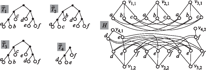
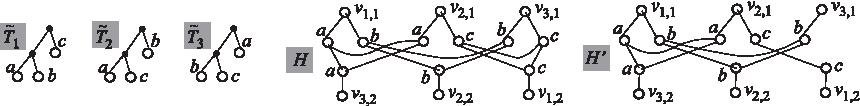
Four trees $\tilde{T}$ ₁, …, $\tilde{T}$ ₄ and the auxiliary graph H constructed from them in Aho et al.'s algorithm.

FIG. 3.

Three trees $\tilde{T}$ ₁, …, $\tilde{T}$ ₃, the auxiliary graph H constructed from them in Aho et al.'s algorithm, and a minimally connected vertex-induced subgraph H′ of H.

For convenience, we refer to P as the label-partition for $\tilde{T}$ . Alternatively, we can obtain P as follows. First, we construct an auxiliary graph H = (V₁ ∪ V₂, E₁ ∪ E₂ ∪ E₃) from $\tilde{T}$ , where

V₁ consists of the leaves (together with their labels) in the trees in $\tilde{T}$ ;

for each ${\tilde{T}}_{i} \in \tilde{T}$ , V₂ contains two vertices v_i_{, 1} and v_i_{, 2};

for each ${\tilde{T}}_{i} \in \tilde{T}$ and for each leaf x of $\tilde{T}$ _i, if x is a descendant of the left (respectively, right) child of the root in $\tilde{T}$ _i, then E₁ (respectively, E₂) contains the edge {x, v_i_{, 1}} (respectively, {x, v_i_{, 2}});

for every two vertices x and y in V₁, if x and y have the same label, then E₃ contains the edge {x, y}.

For example, H is as shown in Figure 2 if $\tilde{T}$ consists of the trees $\tilde{T}$ ₁, …, $\tilde{T}$ ₄ in Figure 2, whereas H is as shown in Figure 3 if $\tilde{T}$ consists of the trees $\tilde{T}$ ₁, …, $\tilde{T}$ ₃ in Figure 3.

Let K₁, …, K_h be the connected components of H. For each i∈{1, …, h}, let X_i be the set of all $x \in X (\tilde{T})$ such that x is the label of some vertex in V (K_i) ∩ V ₁. Then, one can easily see that P = {X₁, …, X_h}. This new computation of P is more efficient because it uses the trees in $\tilde{T}$ directly rather than using the triplets in $t r (\tilde{T})$ . Indeed, there is an even more efficient way of computing P. To see this, first note that for each $x \in X (\tilde{T})$ , the vertices of H with label x form a clique C_x. Suppose that we modify H by contracting C_x to a single vertex (still with label x) for each $x \in X (\tilde{T})$ . The modified H has the same number of connected components as earlier. Moreover, if we compute P from the connected components of the modified H as earlier, then P should be the same as earlier. Further, instead of constructing H and then modifying it, we can construct the modified H from the trees in $\tilde{T}$ directly in linear time. In this way, P can be computed in linear time because the modified graph H has $O (ℓ + | X (\tilde{T}) |)$ vertices and $O (\sum_{i = 1}^{ℓ} | X ({\tilde{T}}_{i}) |)$ edges. The reason that we prefer H to the modified H is that H makes our analysis in Section 3.3 easier.

3.3. A new algorithm

In this subsection, we present a new algorithm for the parameterized version of AST-LR. So, consider an instance (q, {T₁, …, T_m}) of the problem. Note that X(T₁) = ⋯ = X(T_m). For each i∈{1, …, m}, we call Cole et al.'s algorithm (Cole et al., 2000) to compute d_LR(T_i, T_j) for each j∈{1, …, m}, and then check whether $\sum_{j = 1}^{m} d_{L R} (T_{i}, T_{j}) \leq q$ . If $\sum_{j = 1}^{m} d_{L R} (T_{i}, T_{j}) \leq q$ for at least one i∈{1, …, m}; then, we are done by returning “yes.” The total time taken by the calls of Cole et al.'s algorithm is $O (m^{2} n log n)$ , where n is the number of leaves in each of T₁, …, T_m. So, we may assume that there is no i∈{1, …, m} with $\sum_{j = 1}^{m} d_{L R} (T_{i}, T_{j}) \leq q$ . Then, for each phylogenetic tree T with $\sum_{j = 1}^{m} d_{L R} (T, T_{j}) \leq q$ , we have d_LR(T, T_i) ≥ 1 for every i∈{1, …, m}. Consequently, m ≤ q.

Since our algorithm will be recursive, we need to consider a call originated from the root call [i.e., the call on input (q, {T₁, …, T_m}) after zero or more subsequent calls]. Let $(\hat{q}, {{\hat{T}}_{1}, \dots, {\hat{T}}_{k}})$ be the input to the call. We will maintain the invariant that for each i∈{1, …, k}, there is a j∈{1, …, m} with ${\hat{T}}_{i} = T_{j} |_{X ({\hat{T}}_{i})}$ . So, k ≤ m. However, it is not necessarily true that $X ({\hat{T}}_{1}) = \dots = X ({\hat{T}}_{k})$ . If there is an $i \in {1, \dots, k}$ with $| X ({\hat{T}}_{i}) | \leq 2$ , then we can remove ${\hat{T}}_{i}$ from the input because there is a leaf-disagreement of size at most $\hat{q}$ for $({\hat{T}}_{1}, \dots, {\hat{T}}_{k})$ if and only if there is a leaf-disagreement of size at most $\hat{q}$ for $({\hat{T}}_{1}, \dots, {\hat{T}}_{i - 1}, {\hat{T}}_{i + 1}, \dots, {\hat{T}}_{k})$ . So, we may assume that $| X ({\hat{T}}_{i}) | \geq 3$ for every i∈{1, …, k}.

Let $\hat{T} = {{\hat{T}}_{1}, \dots, {\hat{T}}_{k}}$ . We next detail our algorithm on input $(\hat{q}, \hat{T})$ . In the base case where $\hat{q} < 0$ , the algorithm returns “no.” So, assume that $\hat{q} \geq 0$ . Our algorithm first calls Aho et al.'s algorithm to decide whether there is a phylogenetic tree displaying the trees in $\hat{T}$ . If the call returns “yes,” then our algorithm returns “yes.” Otherwise, as sketched in Section 3.2, the call returns “no” because it has found a set $\tilde{T} = {{\tilde{T}}_{1}, \dots, {\tilde{T}}_{ℓ}}$ of two or more phylogenetic trees satisfying the following conditions:

C1. Each ${\tilde{T}}_{i} \in \tilde{T}$ is a pendant subtree of some ${\hat{T}}_{j_{i}} \in \hat{T}$ with |X( $\tilde{T}$ _i)| ≥ 3.

C2. If i and i′ are different integers in {1, …, ℓ}, then j_i ≠ j_i′.

C3. The partition P of $X (\tilde{T})$ constructed from $t r (\tilde{T})$ is $X (\tilde{T})$ .

For example, if $\hat{T}$ consists of the trees $\tilde{T}$ ₁, …, $\tilde{T}$ ₄ in Figure 2, then a call of Aho et al.'s algorithm on input $\hat{T}$ will return “no” together with $\tilde{T} = {{\tilde{T}}_{1} |_{S_{1}}, \dots, {\tilde{T}}_{3} |_{S_{1}}}$ or $\tilde{T} = {{\tilde{T}}_{1} |_{S_{2}}, \dots, {\tilde{T}}_{4} |_{S_{2}}}$ , where S₁ = {a, b, c} and S₂ = {d, e, f}. Note that by Conditions C1 and C2, ℓ ≤ k ≤ m ≤ q.

Consider the auxiliary bipartite graph H = (V₁ ∪ V₂, E₁ ∪ E₂ ∪ E₃) constructed from $\tilde{T}$ as in Section 3.2. Since $P = X (\tilde{T})$ , H is connected. Our algorithm constructs a vertex-induced subgraph H′ of H as follows. Initially, H′ is a copy of H. Then, as long as H′ has a vertex x∈V₁ such that removing x from H′ does not disconnect H′, we keep modifying H′ by removing x. Suppose that we have finished modifying H′ in this way (see Fig. 3 for an example). Let $V'_{1} = {x \in V_{1} | x s t i l l r e m a i n s i n H'}$ .

Lemma 3.1. $| V'_{1} | \leq 2 | V_{2} | - 2 = 4 ℓ - 2$ .

Proof. Let $E'_{1, 2} = {e \in E_{1} \cup E_{2} | e s t i l l r e m a i n s i n H'}$ . By the construction of H, each $x \in V'_{1}$ is incident to exactly one edge in $E'_{1, 2}$ and each edge in $E'_{1, 2}$ has exactly one endpoint in $V'_{1}$ . Thus, $| V'_{1} | = | E'_{1, 2} |$ . So, it suffices to show that $| E'_{1, 2} | \leq 2 | V_{2} | - 2$ .

Let X′ be the set of labels on the vertices in $V'_{1}$ . Note that for each x∈X′, the vertices of H′ with label x induce a clique K_x in H′. Let H′′ be the graph obtained from H′ by contracting K_x into a single vertex k_x for every x∈X′, where we discard the resulting self-loops but keep the resulting parallel edges. Indeed, H′′ cannot have parallel edges because no vertex in V₂ can be adjacent to two vertices of $V'_{1}$ with the same label in H′. This implies that H′′ has exactly $| E'_{1, 2} |$ edges. Moreover, by the construction of H, H′′ is bipartite. We claim that H′′ has no cycle. For a contradiction, assume that H′′ has a cycle C. Then, since H′′ is bipartite, C contains v₁∈V₂ and v₂∈V₂ such that v₁ and v₂ share a neighbor in C. By the construction of H′′, the common neighbor of v₁ and v₂ in C is obtained by contracting a clique K in H′. For each i∈{1, 2}, K contains exactly one vertex $x_{i} \in V'_{1}$ such that {v_i, x_i} is an edge in H′. By the construction of H′, the neighbors of x₁ in H′ are v₁ and the vertices in K other than x₁ itself. Since both x₁ and x₂ belong to K, they have the same label. So, each neighbor of x₁ in H′ other than v₁ is also a neighbor of x₂ in H′. Now, since v₁ can be reached from x₂ without passing x₁ in C, removing x₁ from H′ does not disconnect H′, a contradiction.

By the claim just made, H′′ is a tree and hence has |X′| + |V₂| − 1 edges. Moreover, each vertex of H′′ not in V₂ cannot be a leaf of H′′ because otherwise, we would be able to remove more vertices of $V'_{1}$ from H′ without disconnecting it. So, |X′| + |V₂| − 1 ≥ 2|X′| and, in turn, |X′| ≤ |V₂| − 1. Thus, H′′ has at most 2(|V₂| − 1) edges. Therefore, $| E'_{1, 2} | \leq 2 (| V_{2} | - 1)$ . ▪

For each i ∈{1, …, ℓ}, let $V'_{1, i} = {x \in V'_{1} | x$ is a leaf of $\tilde{T}$ _i} and $\tilde{T}'_{i} = {\tilde{T}}_{i} |_{{V'}_{1, i}}$ .

Lemma 3.2. There is no phylogenetic tree displaying the trees in $\tilde{T}' = {\tilde{T}'_{i} | V'_{1, i} \neq \emptyset}$ .

Proof. If we construct an auxiliary graph from $\tilde{T}'$ in the same way as we construct H from $\tilde{T}$ in Section 3.2, then the graph will be exactly H′ and, in turn, be connected. Moreover, if we call Aho et al.'s algorithm on input $(X (\tilde{T}'), t r (\tilde{T}'))$ , then it will compute a partition P′ of $X (\tilde{T}')$ from $t r (\tilde{T}')$ in the same way as it computes the partition P of $X (\tilde{T})$ from $t r (\tilde{T})$ . Since H′ is connected, $P' = {X (\tilde{T}')}$ and, in turn, the correctness of Aho et al.'s algorithm implies that no phylogenetic tree can display the trees in $\tilde{T}'$ .

By Conditions C1 and C2, $\tilde{T}'_{i} = {\hat{T}}_{j_{i}} |_{{V'}_{1, i}}$ as well for each $\tilde{T}'_{i} \in \tilde{T}'$ . Thus, by Lemma 3.2, we need to delete at least one leaf of $V'_{1}$ from some ${\hat{T}}_{j_{i}}$ with $\tilde{T}'_{i} \in \tilde{T}'$ , to make the trees in ${{\hat{T}}_{j_{i}} | \tilde{T}'_{i} \in \tilde{T}'}$ compatible. For convenience, we refer to $V'_{1}$ as a small witness for the incompatibility of the trees in $\hat{T}$ . Now, for each i∈{1, …, ℓ} and for each leaf x in $\tilde{T}'_{i}$ , our algorithm makes a recursive call on input $(\hat{q} - 1, {{\hat{T}}_{1}, \dots, {\hat{T}}_{j_{i} - 1}, {\hat{T}}_{j_{i}} - {x}, {\hat{T}}_{j_{i} + 1}, \dots, {\hat{T}}_{k}})$ . If at least one of the calls returns “yes,” then the algorithm returns “yes”; otherwise, it returns “no.”

To compute $V'_{1}$ from $\tilde{T}$ efficiently, we can proceed as follows.

Try to find an x such that x is a proper leaf descendant of a child of the root of some $\tilde{T}$ _i with i∈{1, …, ℓ} and the label-partition for ${{\tilde{T}}_{1}, \dots, {\tilde{T}}_{i - 1}, {\tilde{T}}_{i} - {x}, {\tilde{T}}_{i + 1}, \dots, {\tilde{T}}_{ℓ}}$ is the same as that for { $\tilde{T}$ ₁, …, $\tilde{T}$ _ℓ}. (Comment: As noted in Section 3.2, the label-partition can be computed in linear time.)

If x is found in Step 1, then remove it from $\tilde{T}$ _i and go to Step 1. Otherwise, set $V'_{1}$ to be the set of leaves in $\tilde{T}$ ₁, …, $\tilde{T}$ _ℓ.

So, $V'_{1}$ can be computed in quadratic time.

Theorem 3.3. The parameterized version of AST-LR for input (q, {T₁, …, T_m}) can be solved in $O ({(4 q - 2)}^{q} m^{2} n^{2})$ time, where n is the number of leaves in each input tree.

Proof. It takes $O (m^{2} n log n)$ time to check whether some T_i with i∈{1, …, m} is a size-q center tree for {T₁, …, T_m}. If it is, we are done. So, assume that no T_i with i ∈{1, …, m} is a size-q center tree for {T₁, …, T_m}. By Lemma 3.1, the total number of recursive calls made by the algorithm is at most (4q − 2)^q. In each recursive call, if we exclude the time needed by subsequent recursive calls, the most time-consuming processing is to call Aho et al.'s algorithm to decide whether the current trees are compatible, and to further find a small witness whether they are incompatible. This processing can be done in O(m²n²) time as noted earlier.

In Figure 4, we summarize our algorithm for the parameterized version of AST-LR.

FIG. 4.

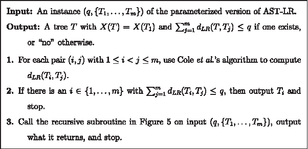
The algorithm for the parameterized version of AST-LR.

FIG. 5.

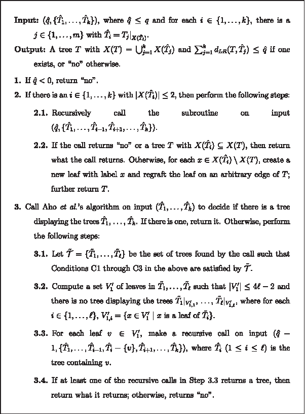
A recursive subroutine called by the algorithm in Figure 4 on input (q, {T₁, …, T_m}).

4. Integer-Linear Programming Approach to AST-LR and AST-LR-d

For convenience, we use the notation (j₁, …, j_k) ⊆ S to denote an ordered subset (j₁, …, j_k) of a set S. Let $T = {T_{1}, \dots, T_{m}}$ be a set of phylogenetic trees not necessarily with X(T₁) = ⋯ = X(T_m). A quadruple $(x_{j}, x_{k}, x_{l}, x_{h}) \subseteq X (T)$ is inconsistent in $T$ if

${x_{j} x_{k} | x_{l}, x_{l} x_{h} | x_{k}, x_{k} x_{h} | x_{j}} \subseteq t r (T)$

${x_{j} x_{k} | x_{l}, x_{l} x_{h} | x_{k}, x_{j} x_{h} | x_{k}} \subseteq t r (T) .$

The following lemma is well known and will be useful for constructing ILP models for AST-LR and AST-LR-d.

Lemma 4.1. A full set $T$ of triplets is compatible if and only if no quadruple $(x_{j}, x_{k}, x_{l}, x_{h}) \subseteq X (T)$ is inconsistent in $T$ .

4.1. Exact integer-linear programming models

We first show an ILP model for AST-LR-d. So, let (d, {T₁, …, T_m}) be an instance of the problem. Let $T = {T_{1}, \dots, T_{m}}$ . Note that X(T₁) = ⋯ = X(T_m). Let x₁, …, x_n be the elements in $X (T)$ . Suppose that we want to remove a set of leaves from each T_i so that there is a center tree T displaying the resulting trees. For this purpose, we introduce a binary variable y_i_,j for each i∈{1, …, m} and each j∈{1, …, n}. The value of y_i_{, j} is supposed to be 1 if and only if we delete the leaf with label x_j from T_i. For each (j, k, l) ⊆ {1, …, n}, we define I_j_,k,l,0 = {i∈{1, …, m} | T_i|_{xj,xk,xl} = x_jx_k|x_l}, I_j_,k,l,1 = {i∈{1, …, m} | T_i|_{xj,xk,xl} = x_jx_l|x_k}, and I_j_{,k,l, 2} = {i∈{1, …, m} | T_i|_{xj,xk,xl} = x_kx_l|x_j}; moreover, we introduce two binary variables a_j_,k,l and b_j_,k,l. The values of a_j_,k,l and b_j_{, k, l} are supposed to be as follows.

a_j_,k,l = 0 and b_j_,k,l = 0 if and only if T|_{xj,xk,xl} = x_jx_k|x_l.

a_j_,k,l = 0 and b_j_,k,l = 1 if and only if T|_{xj,xk,xl} = x_jx_l|x_k.

a_j_,k,l = 1 and b_j_,k,l = 0 if and only if T|_{xj,xk,xl} = x_kx_l|x_j.

We also introduce an integral variable d whose value is supposed to be an upper bound on the radius of a leaf-disagreement for {T₁, …, T_m}. Then, our ILP problem for AST-LR-d is as follows:

Minimize d

Subject to $\begin{matrix} \forall_{1 \leq i \leq m} \sum_{j = 1}^{n} y_{i, j} \leq d \\ \forall_{(j, k, l) \subseteq {1, \dots, n}} a_{j, k, l} + b_{j, k, l} \leq 1 \\ \forall_{(j, k, l) \subseteq {1, \dots, n}} \forall_{i \in I_{j, k, l, 0}} y_{i, j} + y_{i, k} + y_{i, l} \geq a_{j, k, l} + b_{j, k, l} \\ \forall_{(j, k, l) \subseteq {1, \dots, n}} \forall_{i \in I_{j, k, l, 1}} y_{i, j} + y_{i, k} + y_{i, l} \geq 1 - b_{j, k, l} \\ \forall_{(j, k, l) \subseteq {1, \dots, n}} \forall_{i \in I_{j, k, l, 2}} y_{i, j} + y_{i, k} + y_{i, l} \geq 1 - a_{j, k, l} \\ \forall_{(j, k, l, h) \subseteq {1, \dots, n}} a_{j, k, l} + b_{j, k, l} - a_{k, l, h} - a_{j, k, h} \geq - 1 \\ \forall_{(j, k, l, h) \subseteq {1, \dots, n}} a_{j, k, l} + b_{j, k, l} - a_{k, l, h} - b_{j, k, h} \geq - 1 \\ \forall_{1 \leq i \leq m} \forall_{1 \leq j \leq n} y_{i, j} \in {0, 1} \\ \forall_{(j, k, l) \subseteq {1, \dots, n}} a_{j, k, l} \in {0, 1} \\ \forall_{(j, k, l) \subseteq {1, \dots, n}} b_{j, k, l} \in {0, 1} \end{matrix}$ (4.1)

The constraints can be understood as follows:

The first set of constraints requires that the maximum number of leaves removed from each tree T_i in the output leaf-disagreement is at most d.

The second set of constraints requires that for each (j, k, l) ⊆ {1, …, n}, the output center tree T contains exactly one of the triplets x_jx_k|x_l, x_jx_l|x_k, and x_kx_l|x_j.

The third set of constraints requires that for each (j, k, l) ⊆ {1, …, n}, if T_i contains the triplet x_jx_k|x_l but the output center tree T does not, then at least one of x_j, x_k, and x_l should be removed from T_i.

The fourth set of constraints requires that for each (j, k, l) ⊆ {1, …, n}, if T_i contains the triplet x_jx_l|x_k but the output center tree T does not, then at least one of x_j, x_k, and x_l should be removed from T_i.

The fifth set of constraints requires that for each (j, k, l) ⊆ {1, …, n}, if T_i contains the triplet x_kx_l|x_j but the output center tree T does not, then at least one of x_j, x_k, and x_l should be removed from T_i.

The sixth and the seventh sets of constraints are based on Lemma 4.1. Moreover specifically, the sixth set of constraints requires that at least one of the triplets x_jx_k|x_l, x_lx_h|x_k, x_kx_h|x_j should not appear in the output center tree T, whereas the seventh set of constraints requires that at least one of the triplets x_jx_k|x_l, x_lx_h|x_k, x_jx_h|x_k should not appear in the output center tree T.

To obtain an ILP model for AST-LR, we just simply modify the ILP model cited earlier for AST-LR-d by deleting the first set of constraints and replacing the objective function d with $\sum_{i = 1}^{m} \sum_{j = 1}^{n} y_{i, j}$ .

4.2. Relaxed integer-linear programming models

The ILP models in Section 4.1 are exact in the sense that they solve AST-LR-d and AST-LR exactly. Unfortunately, since the models contain too many constraints, they may take long a time to be solved by an ILP solver (such as Gurobi and Cplex). So, we next propose relaxed ILP models instead; the relaxed model for AST-LR-d (respectively, AST-LR) alone does not solve AST-LR-d (respectively, AST-LR) but will be used to speed up solving the exact model for AST-LR-d (respectively, AST-LR).

As stated earlier, we first present a relaxed ILP model for AST-LR-d and then modify it into a relaxed ILP model for AST-LR. The idea behind our relaxed ILP model for AST-LR-d is to avoid computing the triplets T|_{xj,xk,xl} in the output center tree T. Intuitively speaking, the idea is to remove the variables a_j_,k,l and b_j_,k,l from the exact models. Without knowing the triplet T|_{xj,xk,xl}, we have to resort to removing direct conflicts between the input trees. In other words, for every (j,k,l) ⊆ {1, …, n} and for every ${i_{1}, i_{2}} \subseteq {1, \dots, m}$ , if T_i₁|_{xj,xk,xl} and T_i₂|_{xj,xk,xl} are different, we add the constraint $y_{i_{1}, j} + y_{i_{1}, k} + y_{i_{1}, l} + y_{i_{2}, j} + y_{i_{2}, k} + y_{i_{2}, l} \geq 1$ to the model. Similarly, for every $(j, k, l, h) \subseteq {1, \dots, n}$ and for every {i₁,i₂,i₃} ⊆ {1, …, m}, if one of the following holds, then we add the constraint $y_{i_{1}, j} + y_{i_{1}, k} + y_{i_{1}, l} + y_{i_{2}, k} + y_{i_{2}, l} + y_{i_{2}, h} + y_{i_{3}, j} + y_{i_{3}, k} + y_{i_{3}, h} \geq 1$ to the model:

T_i₁|_{xj,xk,xl} = x_jx_k|x_l, T_i₂|_{xk,xl,xh} = x_lx_h|x_k, and T_i₃|_{xj,xk,xh} = x_kx_h|x_j.

T_i₁|_{xj,xk,xl} = x_jx_k|x_l, T_i₂|_{xk,xl,xh} = x_lx_h|x_k, and T_i₃|_{xj,xk,xh} = x_jx_h|x_k

In summary, we have obtained the following relaxed ILP model for AST-LR-d:

Minimize d

Subject to $\begin{matrix} \forall_{1 \leq i \leq m} \sum_{j = 1}^{n} y_{i, j} \leq d \\ \forall_{(j, k, l) \subseteq {1, \dots, n}} \forall_{{t_{1}, t_{2}} \subseteq {0, 1, 2}} \forall_{i_{1} \in I_{j, k, l, t_{1}}} \forall_{i_{2} \in I_{j, k, l, t_{2}}} \\ y_{i_{1}, j} + y_{i_{1}, k} + y_{i_{1}, l} + y_{i_{2}, j} + y_{i_{2}, k} + y_{i_{2}, l} \geq 1 \\ \forall_{(j, k, l, h) \subseteq {1, \dots, n}} \forall_{i_{1} \in I_{j, k, l, 0}} \forall_{i_{2} \in I_{k, l, h, 2}} \forall_{i_{3} \in I_{j, k, h, 1} \cup I_{j, k, h, 2}} \\ y_{i_{1}, j} + y_{i_{1}, k} + y_{i_{1}, l} + y_{i_{2}, k} + y_{i_{2}, l} + y_{i_{2}, h} + y_{i_{3}, j} + y_{i_{3}, k} + y_{i_{3}, h} \geq 1 \\ \forall_{1 \leq i \leq m} \forall_{1 \leq j \leq n} y_{i, j} \in {0, 1} \end{matrix}$ (4.2)

To obtain a relaxed ILP model for AST-LR, it suffices to modify the relaxed ILP model cited earlier for AST-LR-d by deleting the first set of constraints and replacing the objective function d with $\sum_{i = 1}^{m} \sum_{j = 1}^{n} y_{i, j}$ .

4.3. Using the relaxed models to speed up the exact models

Here, we only explain how to use the relaxed model of AST-LR-d to speed up solving its exact counterpart. Similar discussions apply to the models of AST-LR as well.

By experiments, we have found that the relaxed model for AST-LR-d can be solved much faster than its exact counterpart by Gurobi or Cplex. Of course, an optimal solution s* of the relaxed model may not lead to a correct leaf-disagreement. In more details, even though s* tells us which leaves should be removed from each input tree T_i, there may not exist a center tree displaying all the resulting trees after the removals. Nevertheless, instead of solving the exact model directly, we can first solve the relaxed model to obtain s* and then proceed to solving the exact model with the help of s*. The crucial points are as follows:

The value of d in s* is a lower bound on the optimal objective value of the exact ILP model. We can incorporate this bound into the exact model when solving it with an ILP solver. The bound can help the solver prune a lot of unnecessary branches of the search tree.

The values of y_i_{, j'}s in s* can be used as a starting partial-solution when solving the exact model by an ILP solver. By experiments, we have found that the partial start can often be extended to a feasible (and hence optimal) solution of the corresponding exact model by the solver. As the result, the solver can often solve the exact model within almost the same time as the relaxed model.

As will be seen in Section 4.4, using the relaxed model as cited earlier leads to significant speedup of solving the exact model.

4.4. Experimental results

To evaluate our ILP models empirically, we run our program on a Ubuntu (x64) desktop PC with i7-4790K CPU and 31.4 GiB RAM and another CentOS (x64) desktop PC with E5-2687W(v4) CPU and 252.2 GiB RAM. We used two machines instead of a single machine in our experiments just for the sake of finishing the experiments sooner. To solve our ILP models, we use Gurobi as the solver.

Our (exact or relaxed) models have many constraints and, hence, it often takes time for Gurobi to get started. Note that most of the constraints are for excluding inconsistent quadruples. In our experiments, we use these constraints as lazy constraints when using Gurobi to solve the models. In greater detail, Gurobi will remove these constraints at the beginning, but will add an initially removed constraint back later if the constraint is found to be violated by the incumbent integral solution. In this way, Gurobi can start up much faster. Moreover, by experiments, we have found that a set of trees without inconsistent triples often have no inconsistent quadruples. Thus, we can often expect that very few initially removed constraints are added back and, in turn, Gurobi can finish within a much shorter time.

To test the performance of our models, we generate simulated datasets as follows. First, for each n∈{15, 25}, we use a program due to Beiko and Hamilton (2006) to generate a set $S_{n}$ of 100 random phylogenetic trees with n leaves. Then, for each n∈{15, 25}, each $T \in S_{n}$ , and each k∈{1, 3, 5, 7}, we generate five trees T_n_,k,1, …, T_n_,k,5 from T by performing k random nearest-neighbor interchange moves on T; the trees T_n_,k,1, …, T_n_,k,5 together form an instance of AST-LR and AST-LR-d. So, in total, there are 800 instances in our experiment for each of AST-LR and AST-LR-d. Since there are many instances and some of them may take a long time to solve, we use the Ubuntu (respectively, CentOS) machine for those instances with n = 15 (respectively, n = 25).

Our experimental results for AST-LR-d and AST-LR are summarized in Tables 1 and 2, respectively. From the tables, one can see that compared with solving the exact model directly, it is much faster to first solve the relaxed model and then use its output to solve the exact model. Moreover, in case both of the methods fail to find optimal solutions within the time limit, the latter method finds better approximate solutions.

Table 1.

Experimental Results for AST-LR-d

#leaf	#nni	Exact-only		Rlx+Exact		Both-fail
		Time	#fail	Time	#fail	#inst	Radius
		Time	#fail	Time	#fail	#inst	Exact-only	Rlx+Exact
15	1	0.409	0	0.156	0	0	0	0
	3	204.006	3	1.515	0	0	0	0
	5	1651.191	37	93.553	4	0	0	0
	7	2281.812	57	367.732	18	14	7.857	6.929
25	1	81.650	0	1.952	0	0	0	0
	3	277.068	4	27.409	2	0	0	0
	5	1744.218	41	235.581	6	4	20.0	8.75
	7	3268.389	87	950.412	24	23	21.870	9.087

Column #leaf indicates the number of leaves in a single input tree, #nni indicates the number of nearest-neighbor interchange moves used to obtain a single input tree from a simulated center tree, Time indicates the average time in seconds, #fail indicates the number of instances for which Gurobi fails to find an optimal solution within the time limit (1 hour), #inst indicates the number of instances, Exact-only indicates solving the exact model only with a 1-hour time limit, Rlx+Exact indicates solving the relaxed model first with a 40-minute time limit and then using its output to solve the exact model with a 20-minute time limit, and Both-fail indicates both Exact-only and Rlx+Exact fail to find an optimal solution within the time limit.

Table 2.

Experimental Results for AST-LR

#leaf	#nni	Exact-only		Rlx+Exact		Both-fail
		Time	#fail	Time	#fail	#inst	Size
		Time	#fail	Time	#fail	#inst	Exact-only	Rlx+Exact
15	1	0.137	0	0.123	0	0	0	0
	3	17.260	0	24.787	2	0	0	0
	5	1394.308	35	147.161	8	3	23.0	23.333
	7	2525.293	64	773.672	23	20	34.95	26.7
25	1	0.548	0	1.381	0	0	0	0
	3	19.270	0	2.280	0	0	0	0
	5	710.779	15	143.081	3	2	117.5	38.5
	7	3024.02	79	1293.147	34	31	105.903	38.613

The columns mean the same as in Table 1.

To evaluate the performance of our ILP models, we have also implemented Chauve et al.'s algorithm (Chauve et al., 2017) for a much simpler parameterized problem (than the parameterized version of AST-LR), where we are only required to decide whether we can delete a total number of at most q leaves from the input trees so that the resulting trees have no conflicting triplets. By experiments, we have found out that the implemented algorithm always takes much longer time than Gurobi solves our ILP models for AST-LR. Because of this clear superiority of our ILP models, we omit our experimental results on the implemented algorithm.

Footnotes

Author Disclosure Statement

The authors declare they have no competing financial interests.

Funding Information

Z.-Z.C. was supported in part by the Grant-in-Aid for Scientific Research of the Ministry of Education, Science, Sports and Culture of Japan, under Grant No. 18K11183. L.W. was supported by a GRF grant from Hong Kong SAR government Project No. [CityU 11256116] and a grant from the National Foundation of China Project No. [61373048].

References

Aho

A.V.

, Sagiv

, Szymanski

T.G.

, et al. 1981. Inferring a tree from lowest common ancestors with application to the optimization of relational expressions. SIAM J. Comput. 10, 405–421.

Baroni

, Grunewald

, Moulton

, et al. 2015. Bounding the number of hybridisation events for a consistent evolutionary history. J. Math. Biol. 51, 171–182.

Beiko

R.G.

, and Hamilton

2006. Phylogenetic identification of lateral genetic transfer events. BMC Evolut. Biol. 6, 15.

Bordewich

, and Semple

2005. On the computational complexity of the rooted subtree prune and regraft distance. Ann. Comb. 8, 409–423.

Buneman

1971. The recovery of trees from measures of dissimilarity, 387–395. In Kendall

., and Tauta

, eds. Mathematics in the Archaeological and Historical Sciences. Edinburgh University Press, Edinburgh.

Chauve

, Jones

, Lafond

, et al. 2017. Constructing a consensus phylogeny from a leaf-removal distance (extended abstract), 129–143. In Proceedings of the 24th International Symposium on String Processing and Information Retrieval, Lecture Notes in Computer Science, vol. 10508. Full version can be found at CoRR abs/1705.05295.

Chen

Z.-Z.

, Fan

, and Wang

2015. Faster exact computation of rSPR distance. J. Comb. Optim. 29, 605–635.

Chen

Z.-Z.

, Harada

, Nakamura

, et al. 2017. Faster exact computation of rSPR distance via better approximation. IEEE/ACM Trans Comput Biol Bioinform, to appear. DOI: 10.1109/TCBB.2018.2878731

Cole

, Farach-Colton

, Hariharan

, et al. 2000. An

O (n log n)

algorithm for the maximum agreement subtree problem for binary trees. SIAM J. Comput. 30, 1385–1404.

10.

Hein

, Jiang

, Wang

, et al. 1996. On the complexity of comparing evolutionary trees. Discrete Appl. Math. 71, 153–169.

11.

Jansson

, Ng

, Sadakane

, et al. 2005. Rooted maximum agreement supertrees. Algorithmica, 43, 293–307.

12.

, Tromp

, and Zhang

1996. On the nearest neighbour interchange distance between evolutionary trees. J. Theor. Biol. 182, 463–467.

13.

, Wang

, and Zhang

1999. Fitting distances by tree metrics with increment error. J. Comb. Optim. 3, 213–225.

14.

, and Zhang

2011. Efficient estimation of the accuracy of the maximum likelihood method for ancestral state reconstruction. J. Comb. Optim. 21, 409–422.

15.

Maddison

W.P.

1997. Gene trees in species trees. Syst. Biol. 46, 523–536.

16.

Nakhleh

, Warnow

, Lindner

C.R.

, et al. 2005. Reconstructing reticulate evolution in species—Theory and practice. J. Comput. Biol. 12, 796–811.

17.

Robinson

, and Foulds

1981. Comparison of phylogenetic trees. Math. Biosci. 53, 131–147.

18.

Schalekamp

, van Zuylen

, and van der Ster

2016. A duality based 2-approximation algorithm for maximum agreement forest, 70:1–70:14. In Proceedings of the 43rd International Colloquium on Automata, Languages, and Programming, Rome Italy. LIPIcs 55, Schloss Dagstuhl-Leibniz-Zentrum fuer Informatik.

19.

Swofford

, Olsen

, Waddell

, et al. 1996. Phylogenetic inference, 407–514. In Hillis

, Moritz

, and Mable

, eds. Molecular Systematics, 2nd ed. Sinauer Associates, Sunderiand.

20.

Whidden

, Beiko

R.G.

, and Zeh

2010. Fast FPT algorithms for computing rooted agreement forest: Theory and experiments. In Proceedings of the 9th International Symposium on Experimental Algorithms. Ischia Island. Naples, Italy. Lecture Notes in Computer Science 6049, 141–153. Springer.