Efficient Estimation and Applications of Cross-Validated Genetic Predictions to Polygenic Risk Scores and Linear Mixed Models

Abstract

Large-scale cohorts with combined genetic and phenotypic data, coupled with methodological advances, have produced increasingly accurate genetic predictors of complex human phenotypes called polygenic risk scores (PRSs). In addition to the potential translational impacts of identifying at-risk individuals, PRS are being utilized for a growing list of scientific applications, including causal inference, identifying pleiotropy and genetic correlation, and powerful gene-based and mixed-model association tests. Existing PRS approaches rely on external large-scale genetic cohorts that have also measured the phenotype of interest. They further require matching on ancestry and genotyping platform or imputation quality. In this work, we present a novel reference-free method to produce a PRS that does not rely on an external cohort. We show that naive implementations of reference-free PRS either result in substantial overfitting or prohibitive increases in computational time. We show that our algorithm avoids both of these issues and can produce informative in-sample PRSs over a single cohort without overfitting. We then demonstrate several novel applications of reference-free PRSs, including detection of pleiotropy across 246 metabolic traits and efficient mixed-model association testing.

1. Introduction

Individual genetic polymorphisms typically explain only a small proportion of the heritability, even for traits that are highly heritable (Nolte et al., 2017). Polygenic risk scores (PRSs) aggregate the contributions of multiple genetic variants to a phenotype (Torkamani et al., 2018). These scores can be calculated using routinely recorded genotypes (Nolte et al., 2017; Torkamani et al., 2018), are strongly associated with heritable traits (Nolte et al., 2017), and are independent of environmental exposures or other factors that are uncorrelated with germ line genetic variants. These properties have motivated a rapidly expanding list of applications from basic science (e.g., causal inference and Mendelian randomization (Burgess and Thompson 2013), hierarchical disease models (Cortes et al., 2017), and identification of pleiotropy (Krapohl et al., 2016) to translation (e.g., estimating disease risk (Maas et al., 2016; Khera et al., 2018), identifying patients who are likely to respond well to a particular therapy (Natarajan et al., 2017), or flagging subjects for modified screening (Seibert et al., 2018).

PRSs are calculated as a weighted sum of genotypes. In some applications, all genotyped single-nucleotide polymorphisms (SNPs) may be used, but often only a small set is given nonzero weight. A subset of SNPs selected to contribute to a PRS may be a genome-spanning-but-uncorrelated LD (Linkage Disequilibrium)-pruned set or a set of SNPs with independent evidence of association with the phenotype of interest. Gene-specific PRSs are also generated using selected sets of SNPs within a region of the genome, such as a window around the coding region of a particular gene (Gamazon et al., 2015; Gusev et al., 2016). The weights on the SNPs included in a polygenic score are often derived from the marginal regression coefficients of an external genome-wide association study (GWAS) (Wray et al., 2007; Dudbridge, 2016), but they may instead be based on predictive models using all SNPs. Joint predictive models include linear mixed models (LMMs) and their sparse extensions (Yang et al., 2011; Zhou et al., 2013; Vilhjálmsson et al., 2015) and other regularized regression models such as the lasso or elastic net (Rakitsch et al., 2012; Warren et al., 2014; Gamazon et al., 2015; Gusev et al., 2016). The predictions from these joint analyses using genome-wide variation are also approximated by postprocessing of GWAS summary statistics (Vilhjálmsson et al., 2015; Gusev et al., 2016).

For these SNP weights to accurately reflect the SNPs' joint association with the phenotype and to generate informative and interpretable PRSs, the reference data set must match the target data set in many ways: the populations must have similar ancestry; the trait of interest must be measured and in a similar way; and identical genotypes must be assayed or imputed. Furthermore, the reference data must be large enough to accurately learn the PRS weights.

An alternative approach is to use the particular data set under consideration to build a reference-free PRS. This eliminates the need for an external reference data set with matched genotypes, phenotypes, and populations. However, as we show below, naive approaches can easily overfit genetic effects. This overfitting results in PRSs correlated with nongenetic components of phenotype, which will induce bias or other errors in downstream applications. Cross-validation is one established approach to mitigate overfitting, which in this context involves holding out and computing a polygenic score for each sample in turn. The main hurdle to this approach is computation time, as standard leave-one-out (LOO) cross-validation requires fitting the PRS model N times in a sample with N individuals.

Here we report an efficient method to generate PRSs using the out-of-sample predictions from a cross-validated LMM. Our approach generates LOO PRSs, which we call cvBLUPs (cross-validated Best Linear Unbiased Predictors), with computational complexity linear in sample size after a single LMM fit. In addition to eliminating the reliance on external data and guaranteeing the PRSs are generated from a relevant population and phenotype, we describe several applications that are only feasible with cvBLUPs. We first demonstrate several desirable statistical properties of cvBLUPs and then consider applications, including evidence of polygenicity across metabolic phenotypes, a novel formulation of mixed model association studies, and selection of relevant principal components for control of confounding by population structure. To facilitate their use, we have incorporated the calculation of cvBLUPs in the genetic analysis program genome-wide complex trait analysis (GCTA) (Yang et al., 2011).

2. Methods

We consider the continuous phenotype y measured on N individuals, which depends on an N-by-M matrix of additively coded genotypes G, other covariates X, and random noise $ε$ : $\begin{matrix} y = X β + G β_{G} + ε \\ ε \sim N (0, σ_{ε}^{2} I_{N}) \end{matrix}$ (1)

For each subject i, the polygenic score PS $_{i}$ is calculated as in Equation 2:

where S is the set of SNPs in the polygenic model, $g_{i j}$ is the number of alleles corresponding to the SNP weights at SNP_j carried by subject i, and ${\hat{β}}_{g, j}$ is the SNP weight. ${\hat{β}}_{g, j}$ is often chosen to be the estimated effect size of SNP j in an external GWAS.

Our objective is to produce an LOO cross-validated polygenic score (PRS) for each subject. We generate our PRS as a genetic prediction from an LMM. LMMs are widely used for genetic prediction (Robinson, 1991), heritability estimation (Kang et al., 2008, 2010; Yang et al., 2010; Lippert et al., 2011; Zhou and Stephens, 2012), and other polygenic analyses (Kang et al., 2008; Lippert et al., 2011; Lee et al., 2012; Zhou and Stephens, 2012). The LMM (Equation 3) jointly models the contributions of all SNPs Z and other covariates X to the phenotype y. Following others (Yang et al., 2011), we define Z by centering and scaling columns of G to have mean 0 and variance 1. $\begin{matrix} y = X β + Z b + ε \\ b \sim N (0, \frac{σ_{g}^{2}}{M} I_{M}) \\ ε \sim N (0, σ_{ε}^{2}) \end{matrix}$ (3)

The key LMM parameters are the genetic variance $σ_{g}^{2}$ and the noise variance $v a r (ε) = σ_{ε}^{2}$ . We estimate these by REML (Patterson and Thompson, 1971; Kang et al., 2008; Yang et al., 2011) or by Haseman–Elston regression (Chen, 2014). These methods can give unbiased estimates of the variance components or heritability even if the genotype matrix Z does not contain the causal SNPs or contains extra, noncausal SNPs as long as the included SNPs adequately “tag” or are correlated with the causal SNPs (Yang et al., 2010). The estimated genetic variance component could be underestimated if the included SNPs do not adequately tag the casual SNPs, and the standard errors of the estimates will increase as more noncausal SNPs are included in the analysis. In some analyses, such as the cvBLUP-adjusted GWAS examples below, additional noncausal SNPs allow better tagging of population or family structure, allowing cvBLUPs to control for confounding in association tests.

These variance estimates are then used to estimate b, the genetic effect sizes (i.e., weights), or Zb, the genetic predictions (i.e., BLUPs):

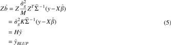
where K is the genetic relatedness matrix computed from the centered and scaled genotypes Z by $K = \frac{1}{M} Z Z^{T}$ . The estimated phenotypic covariance, $\hat{Σ} = {\hat{σ}}_{g}^{2} K + {\hat{σ}}_{ε}^{2} I_{N}$ , where I_N is the N-by-N identity matrix, decomposes the covariance to components due to shared genetics (Zb) and to noise ( $ε$ ).

While the BLUPs in $Z \hat{b}$ could be used as a polygenic score, we show below that this in general overfits the noise ( $ε$ ) and is therefore inappropriate for most PRS applications. To address this problem, we propose to use LOO cross-validated BLUPs instead of ordinary BLUPs, which guarantees independence between genetic predictions and ɛ. Unfortunately, standard LOO approaches will multiply computational time by a factor of N.

We avoid this penalty by leveraging the fact that for linear models, where fitted values are a linear transformation of phenotypes, $ŷ = H ỹ$ , the LOO prediction errors can be calculated from a single model fit (Hastie et al., 2009). BLUPs from LMMs fall into this category of linear predictors by applying $H : = {\hat{σ}}_{g}^{2} K {\hat{Σ}}^{- 1}$ to $ỹ : = (y - X \hat{β})$ , that is, the phenotype after removing estimated fixed effects.

In more detail, the LOO prediction errors are the differences between the LOO genetic predictions and the observed residual phenotypes after subtracting fixed effects, $e_{i, l o o} = y_{i, l o o} - ỹ_{i}$ . The residuals r are the difference between the BLUPs and the residual phenotypes $r_{i} = Z_{i} \hat{b} - ỹ_{i}$ . For a linear model, these are related by a simple equation (Hastie et al., 2009): $e_{i, l o o} = \frac{r_{i}}{1 - H_{i, i}}$ (6)

where $H_{i, i}$ is the i'th diagonal element of the matrix H. Intuitively, this says that due to overfitting, the in-sample residuals r_i are deflated by $(1 - H_{i, i})$ relatively to their unbiased LOO counterparts.

We can rearrange these expressions to calculate the LOO predictions, or cvBLUPs, given the standard BLUPs, the phenotype residuals $ỹ = y - X \hat{β}$ , and the diagonal elements of the H matrix: $ŷ_{i, c v B L U P} = \frac{ŷ_{i, B L U P} - H_{i, i} ỹ_{i}}{1 - H_{i, i}}$ (7)

Because all of these elements are computed when fitting an LMM, cvBLUPs can be produced with no additional computational complexity.

These cvBLUPs are cross-validated genetic predictions or PRSs calculated without using an external reference data set to identify relevant SNPs or to set their weights in the PRS model. Additional or external observations may be assigned PRSs using the data set where the cvBLUPs are calculated as a reference, using the standard BLUP effect size estimates in Equation 4 as SNP weights.

3. Results

3.1. Empirical confirmation of cross-validated predictions

To examine the properties of the proposed cvBLUP formulation, we conducted a set of simulations. We generated 1000 data sets with $N = 1000$ subjects under the model $y = X β + g β_{g} + Z b + ε$ . X consists of five normally distributed covariates and $X β$ jointly explain 20% of the phenotypic variance. g represents an additively coded SNP with allele frequency 0.5, and $g β_{g}$ contributes 2% of the phenotypic variance. Z represents $M = 1000$ independent SNPs with minor allele frequencies drawn i.i.d. and uniformly from [0.05, 0.5]. Effect sizes b_j are drawn i.i.d. from $N (0, \frac{σ_{g}^{2}}{M})$ with the genetic variance $σ_{g}^{2}$ accounting for 39% of the phenotypic variance. The residual noise $ε \sim N (0, σ_{ε}^{2})$ also accounts for 39% of the phenotypic variance, giving a heritability $h^{2} \approx 50 %$ . For each simulated data set, we first estimate variance components and then compute BLUPs and cvBLUPs as described above.

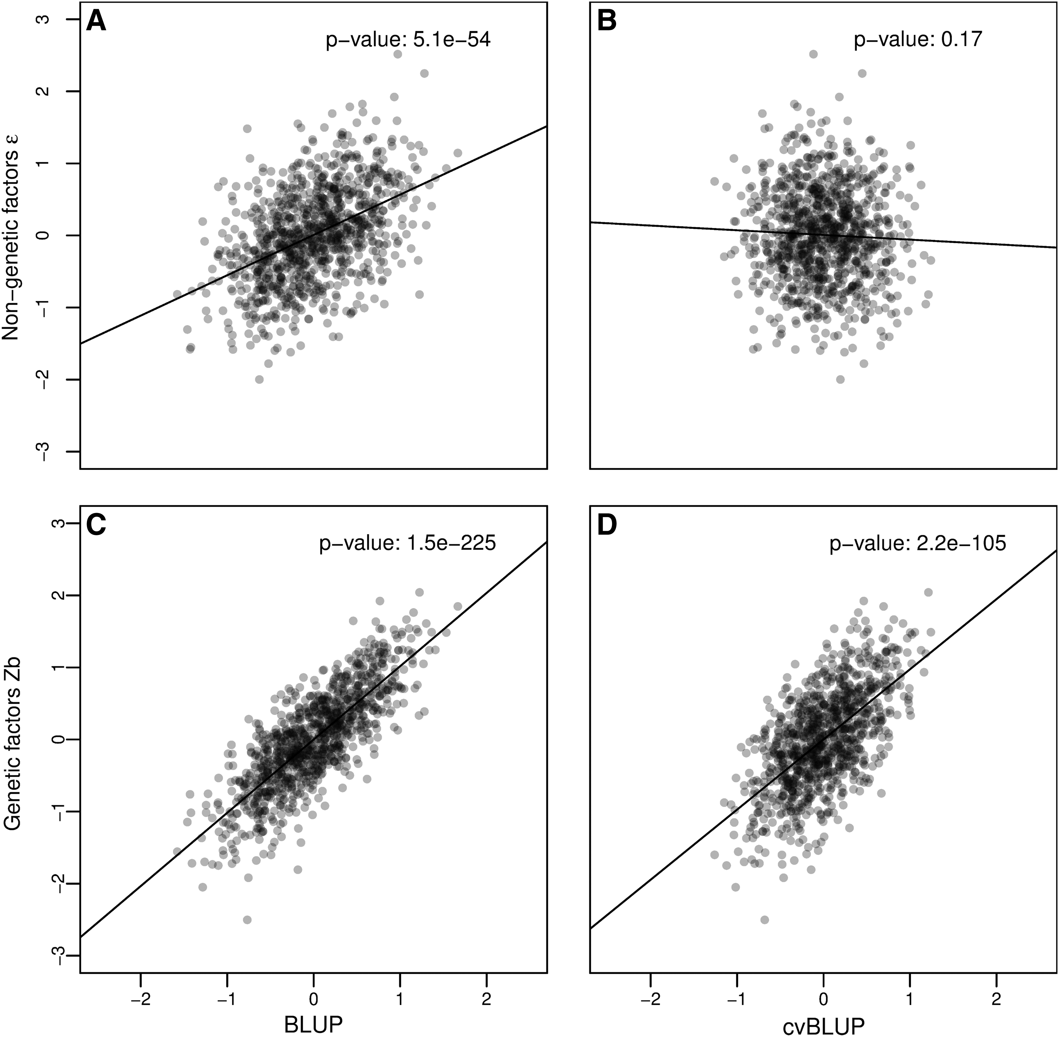
Figure 1 shows scatter plots for one simulation of nongenetic ( $ε$ ) and genetic factors (Zb) plotted against in-sample BLUPs (Left) and cvBLUPs (Right). As expected, the standard BLUPs are highly correlated with $ε$ , but the cvBLUPs are not, a central required property of genetic predictors for most applications. In contrast, both BLUPs and cvBLUPs are highly correlated with the true Zb, emphasizing the subtlety in constructing valid PRSs. See Supplementary Fig S1 for additional details and comparison with k-fold cross-validation.

FIG. 1.

Independence of cvBLUPs and nongenetic factors. Correlations of genetic predictions, BLUPs and cvBLUPs, true genetic factors Zb, and independent environmental factors $ε$ in a simulation of a continuous phenotype with $h^{2} \approx 50 %$ , 1000 subjects, and 1000 independent SNPs having random effect sizes. BLUPs are correlated with $ε$ , while cvBLUPs are not. Lines and p-values are from linear regression fits. R² values: A:0.21, B:0.0019, C:0.64, D:0.38. BLUPs, Best Linear Unbiased Predictors; cvBLUPs, cross-validated Best Linear Unbiased Predictors; SNP, single-nucleotide polymorphism.

Table 1 shows the mean correlations of true simulated values with standard BLUPs and cvBLUPs. Again, standard BLUPs are clearly correlated with the noise term ɛ due to overfitting, but cvBLUPs are appropriately uncorrelated with $ε$ . Standard BLUPs, but not cvBLUPs, are also correlated with the unmodeled causal SNP.

Table 1.

Mean Correlations (and Standard Errors) of BLUPs and cvBLUPs with Each Component of the Additive Simulation Model, $y = X β + g β_{g} + Z b + ε$

	BLUP	cvBLUP
y	0.8241 (0.0013)	0.4058 (0.0013)
$X β$	0.0004 (0.0007)	0.0005 (0.0009)
Zb	0.7884 (0.0005)	0.6212 (0.0008)
$ε$	0.4749 (0.0008)	0.0009 (0.0012)
Unmodeled causal SNP	0.0840 (0.0010)	0.0009 (0.0010)
Unmodeled null SNP	0.0006 (0.0010)	0.0012 (0.0010)

Statistically significant correlations ( $α = 0.05$ ) in bold face.

BLUPs, Best Linear Unbiased Predictors; cvBLUPs, cross-validated Best Linear Unbiased Predictors; SNP, single-nucleotide polymorphism.

This type of correlation causes downstream problems for residual analyses, predictions, and causal inference. Importantly, the cvBLUPs are independent of all unmodeled effects as desired.

3.2. Genetic predictions and cross-trait predictions using cvBLUPs

We next applied cvBLUP in an analysis of Finnish men from the metabolic syndrome in men (METSIM) cohort (Laakso et al., 2017). This cohort comprised 10,197 men aged 45 to 73 at recruitment between 2005 and 2010 in Kuopio, Finland. Blood serum samples were collected from each participant, and 228 metabolites in the samples were quantified by nuclear magnetic resonance spectroscopy (NMR). In addition to the metabolites, biometric traits, including height and weight, and epidemiological traits such as diagnoses or family history of diabetes and coronary heart disease (CHD) were recorded for a total of 248 phenotypes. Continuous phenotypes were quantile normalized. All samples were genotyped at 665,478 SNPs on the Illumina OmniExpress chip. After removing subjects with missing rates above 5% and SNPs with missing rates above 5%, 10,070 subjects and 609,131 SNPs remain.

We initially consider genetic predictions of the metabolic, biometric, and epidemiological traits in an unrelated subset of subjects (with genetic relatedness less than 0.05). Since the metabolic traits are expected to be affected by statins and by pharmaceutical interventions for diabetes, we exclude subjects with diabetes or who use statins from the initial analysis and calculation of cvBLUPs. There are no comparable data sets with the set of metabolic measurements available in the METSIM cohort, but cvBLUPs allow computationally efficient genetic predictions of all 246 phenotypes (excluding diabetes status and statin use). With the genetic prediction models learned in the restricted set of subjects, we extended predictions to the excluded subjects with standard BLUP effect-size estimates (Equation 4). Thus, cvBLUPs allow analyses of reference-free genetic predictions in a subset of subjects that is restricted to avoid confounding by known environmental exposures (statins and responses to diagnoses of diabetes) or by family structure; and these genetic predictions may then be extended to subjects who are initially excluded to avoid confounding.

We first estimated $σ_{g}^{2}$ and $σ_{ε}^{2}$ for each phenotype using LMMs (Yang et al., 2011). Overall, 198 of 246 phenotypes have statistically significant heritability at the 0.05 significance level by Wald tests. The significant heritabilities range from 14.6% to 46.1% with a mean and standard deviation of 27.5% and 8.0%, respectively. The 48 nonsignificant heritabilities range from 0% to 14.4% with a mean and standard deviation of 8.3% and 4.3%, respectively. We next used the method described above to compute LOO PRSs (i.e., cvBLUPs). Figure 2 shows the correlation of the phenotypes (rows) with cvBLUPs (columns) for all 246 phenotypes grouped by hierarchical clustering (Kolde, 2018) of rows and applying the same permutation to columns. The blue diagonal shows the expected positive correlation between a cvBLUP and its own phenotype with mean of 0.065 and standard deviation of 0.037. In the METSIM example all but 7 (of 246) cvBLUP-phenotype pairs are positively correlated, and these exceptional cases are not statistically significantly different than 0.

FIG. 2.

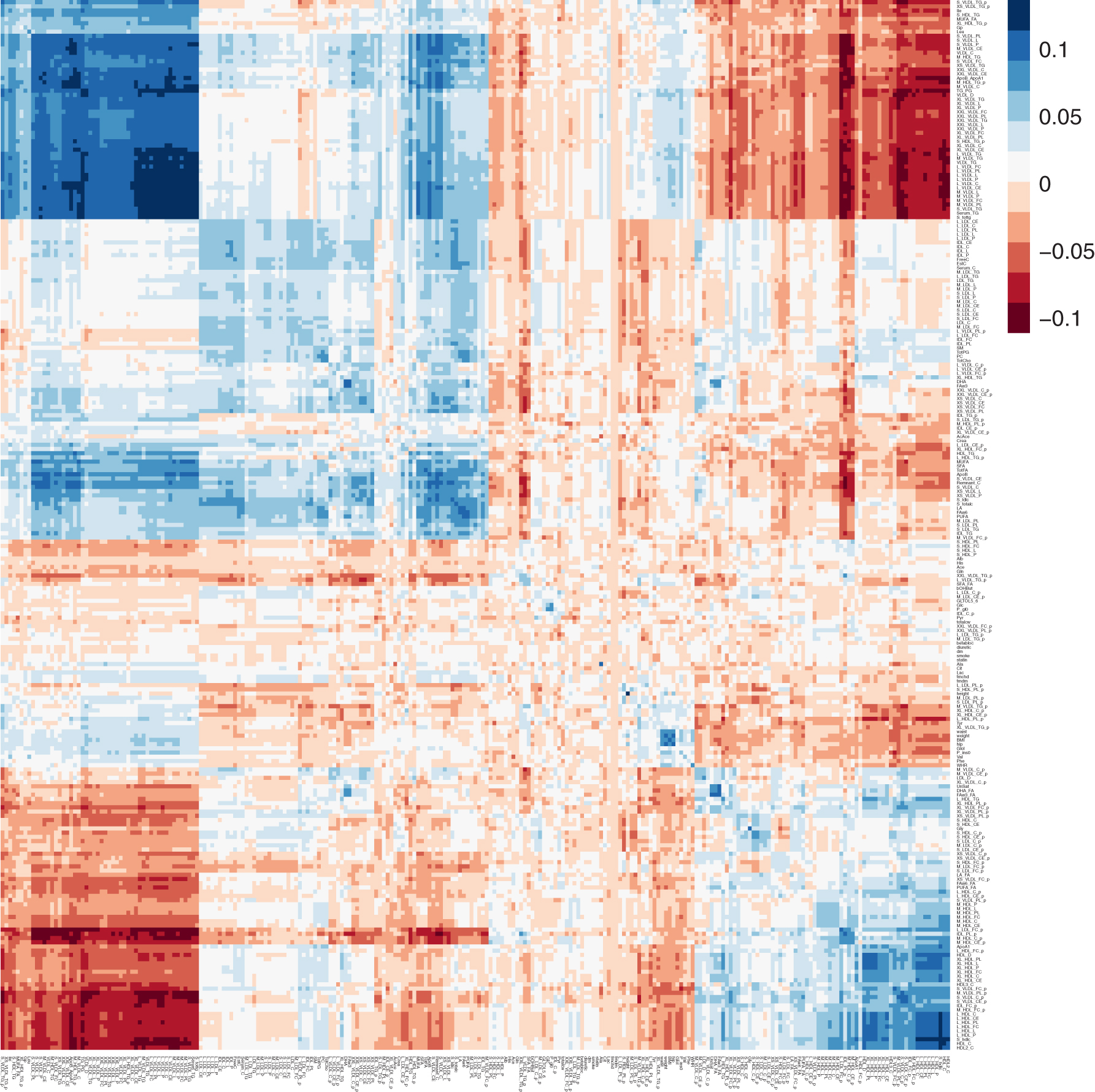
Cross-trait correlations with cvBLUPs. Correlations of phenotypes (rows) and genetic predictions (cvBLUPs, columns) across 246 phenotypes. Many cvBLUPs are strongly correlated with additional phenotypes.

Note that the cvBLUPs are calculated from LMMs that include fixed effects (age, age-squared, and 10 genetic principal components [PCs]). The cvBLUPs are actually genetic predictions for the residual phenotype after projecting out the fixed-effect contributions, and so, there may be cases where the true genetic effect is negatively correlated with the phenotype because of fixed-effect contributions that are negatively correlated with the genetic contributions to the trait. Focusing on the 198 traits with significant heritabilities, the correlations between cvBLUP and phenotype have mean of 0.078 and standard deviation of 0.027. Of the 246 phenotypes, 136 have p-values for significance tests or correlation between cvBLUPs and phenotypes below the Bonferroni-corrected value of 0.05/246 = 0.000203, and 172 correlations are significant at false discovery rate (FDR) = 0.05 (Benjamini and Yekutieli, 2001).

The off-diagonal blue patches in the figure represent cvBLUPs that are positively correlated and predictive of different phenotypes, while red patches represent cvBLUPs that are predictive but negatively correlated with different phenotypes. The off-diagonal correlations show the widespread pleiotropy of genetic effects on metabolism with over 16,203 off-diagonal cvBLUP-phenotype associations at FDR = 0.05 (Benjamini and Yekutieli, 2001). Many cvBLUP-trait correlations are sign-consistent with the respective trait/trait correlations. For example, high-density lipoprotein (HDL) and low-density lipoprotein (LDL) cholesterol are well known be negatively correlated (Terry et al., 1989), and our results demonstrate this is partially due to negative genetic pleiotropy. That is, we observe that SNPs associated with increased LDL are also associated with decreased HDL in aggregate (and vice versa).

3.3. cvBLUPs in association testing

In addition to use in detection of pleiotropy, polygenic modeling is a widely used tool in association testing (Kang et al., 2008; Lippert et al., 2011; Zhou and Stephens, 2012; Yang et al., 2014; Loh et al., 2015), and we therefore consider cvBLUPs in this context. We compare the relative performance of five groups of methods. First, unadjusted regression; second, principal component-adjusted regression; third, standard LMM association tests; fourth, LMM residual-based methods; and fifth, cvBLUP-adjusted regression. Standard LMM-based methods use association tests where the covariance of the observations based on the genetic relatedness of the subjects is estimated and used to calculate effect estimates and test statistics by generalized least squares (Kang et al., 2008; Lippert et al., 2011; Zhou and Stephens, 2012; Yang et al., 2014). The LMM residual-based methods perform association tests on the BLUP residualized phenotypes and possibly genotypes. Then, to try and account for the bias inherent in using the overfit BLUPs, they perform an adjustment step on the resulting test statistics and effect sizes. These methods were pioneered by GRAMMAR/GRAMMAR-γ and include the recent BOLT and BOLT-INF methods (Aulchenko et al., 2007; Svishcheva et al., 2012; Loh et al., 2015).

The typical sources of confounding for associations with germ line genetic markers are population structure, family structure, and batch effects in the data collection (Listgarten et al., 2010). Genetic principal components as adjustment covariates may suffice to control for confounding by population structure or batch effects, but LMMs are often more effective at controlling these sources of confounding (Kang et al., 2010), while also helping to control confounding by family structure and boosting power to detect true associations over standard fixed-effect regression models (Yang et al., 2014). These benefits of LMMs come at the expense of an increased computational burden over standard linear regression.

In GWAS, the statistical significance of each variant g_j is tested individually. Here, the SNP is jointly analyzed with covariates X and the contributions of unmodeled variants contribute to a larger error term $η = Z^{(- j)} b^{(- j)} + ε$ . $\begin{matrix} y = X β + g_{j} β_{g, j} + η \end{matrix}$ (8)

Often a better estimate of the effect size for a particular SNP g_j may be made by accounting for the contributions of the other variants to the phenotype y, and by blocking the effects of confounders of the associations of genotypes and the phenotype—by adjustment with an appropriate set of fixed-effect covariates or other means (Zaitlen et al., 2012a, 2012b; Yang et al., 2014).

Here we demonstrate the use of cvBLUPs as adjustment covariates in a linear regression model that efficiently captures some of the benefits of a standard mixed model association study. To compare the performance of cvBLUP-adjusted analyses to existing methods for association testing under a range of study scenarios, simulations were used. Methods compared were unadjusted linear regression, PC-adjusted linear regression, a standard LMM association test (GCTA), and BOLT association tests. BOLT results were collected both for the infinitesimal genetic model (BOLT-INF) and the sparse causal genetic model (BOLT-LMM). Association tests conducted with cvBLUP adjustment, GCTA, and BOLT were done with leave-one-chromosome-out schemes, in which the variance components, cvBLUPs, and phenotypic predictions and residuals (BOLT) were calculated using only SNPs that are on different chromosomes than the test-SNPs.

In each simulation, data sets were generated with $N = 2000$ subjects under the model $y = X β + g β_{g} + Z b + ε$ . Here X consists of normally distributed covariates drawn to contribute i.i.d. noise to the phenotypes in the independent-subject simulation, but to be correlated with the subjects' ancestral populations in the simulations with population structure and with family in the simulations with confounding by family structure. $X β$ was scaled to contribute 10% of the phenotypic variance. g represents a set of five additively coded causal SNPs with effect sizes $β_{g}$ set to a common fixed value of 0.25. A set of five null SNPs were also drawn but did not contribute to the phenotype y. Z represents $M = 2000$ independent SNPs modeled with random-effect sizes. For simulations run under the infinitesimal genetic model, the random effects b_j were drawn from $N (0, \frac{σ_{g}^{2}}{M} I_{M})$ with the genetic variance $σ_{g}^{2}$ accounting for 40% of the phenotypic variance. For the sparse noninfinitesimal model, a fraction $m_{c} = 2$ % of the SNPs in Z were selected to be causal with effect sizes drawn from $N (0, \frac{σ_{g}^{2}}{M m_{c}} I_{M})$ . The residual noise $ε \sim N (0, σ_{ε}^{2})$ accounts for 40% of the phenotypic variance, giving a heritability $h^{2} \approx 50 %$ . Effect estimates and test statistics produced by the various analysis methods are summarized for 1000 null SNPs and 1000 causal SNPs.

In Table 2, the results of analyzing data sets with independent subjects and an infinitesimal genetic architecture are shown. All methods produced unbiased effect estimates and well-calibrated tests under the null ( $χ_{N u l l}^{2} \approx 1$ ), but the cvBLUP and mixed-model-based methods were more powerful—with greater average test statistics for the causal SNPs. The BOLT effect estimates were biased, with effect sizes deflated toward zero. This deflation of BOLT effect estimates is seen across the simulation scenarios; however, we do not detect deflation of the BOLT effect estimates in the real-data analyses of the METSIM cohort data below, where there are many ratios of counts of SNPs to number of subjects. Bias in BOLT may be due to the empirical estimation of a deflation-correction factor for the residual-based test based on the GRAMMAR- $γ$ adjusted residual analysis method (Svishcheva et al., 2012; Loh et al., 2015). When the true genetic contribution to the phenotype, Zb (not including the test-SNPs), is included as a covariate in a linear regression association test of causal SNPs g, the power is greatly increased.

Table 2.

Simulations with Infinitesimal Genetic Model, Without Population or Family Structure

Model	mean( $β_{g 0}$ )	se( $β_{g 0}$ )	mean( $χ_{N u l l}^{2}$ )	se( $χ_{N u l l}^{2}$ )	mean( $β_{g}$ )	se( $β_{g}$ )	mean( $χ^{2}$ )	se( $χ^{2}$ )
LR	−4.00E-04	1.30E-03	0.99	0.05	0.250	1.30E-03	47.11	0.66
LR + 4 PCs	−5.00E-04	1.30E-03	0.99	0.05	0.250	1.30E-03	46.97	0.66
LR + cvBLUP	−1.30E-03	1.10E-03	1.00	0.05	0.249	1.20E-03	58.53	0.81
LR + BLUP	−1.00E-03	6.00E-04	1.05	0.05	0.096	6.00E-04	36.63	0.56
LMM	−1.30E-03	1.10E-03	1.00	0.05	0.249	1.20E-03	56.62	0.76
BOLT-INF	−1.30E-03	1.00E-03	1.01	0.05	0.219	1.00E-03	56.13	0.76
BOLT-LMM	−1.30E-03	1.00E-03	1.00	0.05	0.219	1.00E-03	56.04	0.75
LR + true genetic effect	−1.00E-03	9.00E-04	1.04	0.05	0.250	9.00E-04	96.28	1.26

Mean and standard error for effect estimates and test statistics of association tests at 1000 null SNPs with true $β_{g 0} : \hat{β_{g 0}}$ and $χ_{N u l l}^{2}$ ; and at 1000 causal SNPs with an alternative hypothesis of true $β_{g} = 0.25$ : ${\hat{β}}_{g}$ and $χ^{2}$ .

LMM, linear mixed model; PC, genetic principal component; BLUP, Best Linear Unbiased Predictor; cvBLUP, cross-validated Best Linear Unbiased Predictor.

In Table 3, the results of analyzing data sets with confounding by population structure are shown. Subjects were drawn from five distinct populations with pairwise Fst set to 0.03. Population-specific allele frequencies were generated by the Balding–Nickels model (Balding and Nichols, 1995). The component $X β$ in the generating model was drawn to be correlated with population, but X was not used in the analyses. In this scenario, unadjusted linear regression and linear regression with fewer than four principal components as adjustment covariates give inflated test statistics and excessive false positives under the null, $χ_{N u l l}^{2} > 1$ . Correcting for population structure by inclusion of four principal components, cvBLUP adjustment, or use of the mixed-model-based methods gives well-calibrated test statistics under the null, $χ_{N u l l}^{2} \approx 1$ . For causal test SNPs, cvBLUP and mixed-model-based methods give greater test statistics than PC-adjusted linear regression with four PCs, indicating greater power. Linear regression with adjustment with the true genetic effect Zb gives high power for detecting causal SNPs, but does not control for inflation of test statistics at null SNPs due to population structure $- χ_{N u l l}^{2} = 3.55 ≫ 1$ . Covariate adjustment with cvBLUPs controls the confounding by population structure and improves the power as do the LMM-based methods. These methods use all SNPs and detect the shifts in allele frequencies across populations when there is confounding by population structure.

Table 3.

Simulations with Infinitesimal Genetic Model and Population Structure

Model	mean( $β_{g 0}$ )	se( $β_{g 0}$ )	mean( $χ_{N u l l}^{2}$ )	se( $χ_{N u l l}^{2}$ )	mean( $β_{g}$ )	se( $β_{g}$ )	mean( $χ^{2}$ )	se( $χ^{2}$ )
LR	−1.2E-03	2.30E-03	2.94	0.14	0.250	2.20E-03	47.28	0.92
LR + 1 PC	−8.00E-04	2.10E-03	2.44	0.12	0.250	1.90E-03	48.20	0.85
LR + 2 PCs	−1.00E-04	1.80E-03	1.94	0.09	0.253	1.70E-03	49.00	0.80
LR + 3 PCs	−3.00E-04	1.60E-03	1.49	0.07	0.252	1.50E-03	48.90	0.76
LR + 4 PCs	1.00E-03	1.30E-03	1.02	0.05	0.250	1.30E-03	47.86	0.70
LR + cvBLUP	4.00E-04	1.20E-03	1.00	0.04	0.240	1.20E-03	56.8	0.81
LMM	−2.00E-04	1.20E-03	0.99	0.05	0.252	1.20E-03	56.97	0.79
BOLT-INF	−1.00E-04	1.00E-03	0.97	0.04	0.214	1.00E-03	54.34	0.76
BOLT-LMM	−1.00E-04	1.00E-03	0.97	0.04	0.214	1.00E-03	54.37	0.76
LR + true genetic effect	2.20E-03	1.80E-03	3.55	0.16	0.250	1.80E-03	89.28	1.56

Mean and standard error for effect estimates and test statistics of association tests at 1000 null SNPs with true $β = g 0 : \hat{β_{g 0}}$ and $χ_{N u l l}^{2}$ ; and at 1000 causal SNPs with an alternative hypothesis of true $β_{g} = 0.25 : {\hat{β}}_{g}$ and $χ^{2}$ .

cvBLUPs correct for population structure because they are weighted combinations of ALL principal components, where weights are based on the singular value corresponding to the principal component and on the strength of the association of the principal component with the outcome (see Supplementary Data). Conceptually, cvBLUPs control for population structure as if all PCs were considered and the most relevant ones for the analysis were kept.

In Table 4, the results of analyzing data sets with confounding by family structure are shown. Here the 2000 subjects in each simulation represented 200 families with 10 subjects each. Families were generated in pedigrees with four founders and six of their descendants, with descendants' genotypes selected independently by drop-down from their parents. In the data-generating model, there were covariate effects correlated with family membership, $X β$ , but these covariates were not included in the analyses, creating confounding by family structure. In this scenario, unadjusted linear regression and PC-adjusted linear regression have inflated test statistics ( $χ_{N u l l}^{2} > 1$ ) and correspondingly high FDRs. Standard LMMs (GCTA) control for the confounding by family structure, with accurate effect estimates ${\hat{β}}_{g}$ under the null and alternate, and barely inflated test statistics under the null $- χ_{N u l l}^{2}$ having mean and standard deviation of 1.10 and 0.05, respectively. In this scenario, cvBLUP-adjusted analyses and the results from BOLT have biased effect estimates under the alternative, and deflated (conservative) test statistics under the null. This suggests overadjustment for family structure in both cvBLUP-adjusted analyses and BOLT.

Table 4.

Simulations with Infinitesimal Model and Family Structure

Model	mean( $β_{g 0}$ )	se( $β_{g 0}$ )	mean( $χ_{N u l l}^{2}$ )	se( $χ_{N u l l}^{2}$ )	mean( $β_{g}$ )	se( $β_{g}$ )	mean( $χ^{2}$ )	se( $χ^{2}$ )
LR	−1.30E-03	1.60E-03	1.52	0.07	0.252	1.60E-03	48.81	0.77
LR + 4 PCs	−5.00E-04	1.50E-03	1.49	0.06	0.253	1.60E-03	48.93	0.75
LR + cvBLUP	4.00E-04	1.00E-03	0.81	0.03	0.183	9.00E-04	36.20	0.52
LMM	5.00E-04	1.40E-03	1.10	0.05	0.251	1.30E-03	48.57	0.68
BOLT-INF	5.00E-04	9.00E-04	0.77	0.03	0.166	9.00E-04	33.65	0.46
BOLT-LMM	5.00E-04	9.00E-04	0.84	0.04	0.166	9.00E-04	36.24	0.51
LR + true genetic effect	5.00E-04	1.00E-03	1.21	0.05	0.252	1.00E-03	98.24	1.31

Mean and standard error for effect estimates and test statistics of association tests at 1000 null SNPs with true $β_{g 0} = 0 : {\hat{β}}_{0}$ and $χ_{N u l l}^{2}$ ; and at 1000 causal SNPs with an alternative hypothesis of true $β_{g} = 0.25 : {\hat{β}}_{g}$ and $χ^{2}$ .

Tables 5, 6, and 7 are analogous to Tables 2, 3, and 4, showing the results of analyses on simulated groups of independent subjects, data sets with population structure, and data with family structure respectively, but the traits analyzed in Tables 5–7 were generated with sparse genetic architectures while those in Tables 2–4 were generated from the infinitesimal model. In Table 5 we see that linear regression with cvBLUP adjustment in a sparse model gives the same effect size estimates and power as the standard linear mixed model (LMM) GTCA.

Table 5.

Simulations with Sparse Genetic Model and Independent Subjects

Model	mean( $β_{0}$ )	se( $β_{0}$ )	mean( $χ_{N u l l}^{2}$ )	se( $χ_{N u l l}^{2}$ )	mean( $β$ )	se( $β$ )	mean( $χ^{2}$ )	se( $χ^{2}$ )
LR	−1.10E-03	1.40E-03	1.14	0.05	0.249	1.30E-03	47.48	0.70
LR + 4 PCs	−9.00E-04	1.40E-03	1.13	0.05	0.249	1.30E-03	47.38	0.68
LR + cvBLUP	−1.10E-03	1.30E-03	1.14	0.05	0.248	1.20E-03	58.15	0.83
LMM	−1.10E-03	1.30E-03	1.14	0.05	0.248	1.20E-03	56.22	0.78
BOLT-inf	−9.00E-04	1.10E-03	1.14	0.05	0.219	1.00E-03	55.81	0.77
BOLT-LMM	−9.00E-04	1.10E-03	1.09	0.05	0.219	1.00E-03	80.99	1.05
LR + true genetic effect	−6.00E-04	1.00E-03	1.13	0.05	0.249	9.00E-04	94.32	1.26

Mean and standard error for effect estimates and test statistics of association tests at 1000 null SNPs with true $β = 0 : {\hat{β}}_{0}$ and $χ_{N u l l}^{2}$ ; and at 1000 causal SNPs with an alternative hypothesis of true $β = 0.25 : \hat{β}$ and $χ^{2}$ .

Table 6.

Simulations with Sparse Genetic Architecture and Population Structure

Model	mean( $β_{0}$ )	se( $β_{0}$ )	mean( $χ_{N u l l}^{2}$ )	se( $χ_{N u l l}^{2}$ )	mean( $β$ )	se( $β$ )	mean( $χ^{2}$ )	se( $χ^{2}$ )
LR	−1.50E-03	2.30E-03	2.88	0.14	0.245	2.20E-03	46.30	0.90
LR + 4 PCs	−6.00E-04	1.30E-03	1.01	0.05	0.248	1.20E-03	46.57	0.66
LR + cvBLUP	−6.00E-04	1.10E-03	0.97	0.05	0.238	1.10E-03	54.76	0.78
LMM	−7.00E-04	1.20E-03	1.00	0.05	0.247	1.20E-03	55.22	0.76
BOLT-inf	−8.00E-04	1.00E-03	0.97	0.05	0.211	1.00E-03	52.78	0.73
BOLT-LMM	−8.00E-04	1.00E-03	1.02	0.05	0.211	1.00E-03	77.75	1.05
LR + true genetic effect	−2.30E-03	1.90E-03	3.65	0.17	0.247	1.90E-03	87.22	1.56

Table 7.

Simulations with Sparse Genetic Architecture and Family Structure

Model	mean( $β_{0}$ )	se( $β_{0}$ )	mean( $χ_{N u l l}^{2}$ )	se( $χ_{N u l l}^{2}$ )	mean( $β$ )	se( $β$ )	mean( $χ^{2}$ )	se( $χ^{2}$ )
LR	1.30E-03	1.60E-03	1.57	0.07	0.248	1.60E-03	47.46	0.73
LR + 4 PCs	1.20E-03	1.60E-03	1.53	0.07	0.248	1.60E-03	47.33	0.73
LR + cvBLUP	1.50E-03	9.00E-04	0.72	0.03	0.184	9.00E-04	35.81	0.49
LMM	2.00E-03	1.30E-03	0.98	0.05	0.249	1.30E-03	47.34	0.64
BOLT-inf	1.30E-03	9.00E-04	0.69	0.03	0.168	8.00E-04	33.39	0.44
BOLT-LMM	1.30E-03	9.00E-04	0.86	0.04	0.168	8.00E-04	64.13	0.79
LR + true genetic effect	1.70E-03	1.00E-03	1.14	0.05	0.250	1.00E-03	93.55	1.21

Finally, we applied these methods to the METSIM data described above. Tables 8 and 9 show results of GWASs for low density lipoprotein cholesterol (LDLc) and high density lipoprotein cholesterol (HDLc) in the METSIM cohort using cvBLUP-adjusted linear regression and comparison methods as in the simulations above. All p-values were GC adjusted for comparison purposes. All mixed-model-based methods, including LR+cvBLUP, were more powerful than standard linear regression. As expected, BOLT-LMM had the highest power due to modeling of noninfinitesimal structure. In this data analysis, unlike in the simulations above, there is no observed evidence of deflation or bias in effect size estimates by BOLT relative to estimates made by standard linear regression or standard LMM effect size estimates (Tables 8 and 9), suggesting that there is not a problem with deflation of effect size estimates in practice.

Table 8.

Genome-Wide Association Study Results for Baseline Low-Density Lipoprotein Cholesterol Using an Unrelated Subset of Subjects from the Metabolic Syndrome in Men Cohort

	LR	LMM	BOLT-INF	BOLT-LMM	cvBLUP
lambdaGC	1.02	1.02	1.02	1.02	1.02
p-values below 1e-06	31	32	32	35	33
Mean ratio of effect size estimates, 1e-06	0.991	1	0.999	0.999	0.998
Standard error in ratio of effect sizes, 1e-06	0.00243	0	0.000561	0.000561	0.00088
p-values below 5e-08	15	15	15	16	16
Mean ratio of effect size estimates, 5e-08	0.996	1	0.998	0.998	0.999
Standard error in ratio of effect sizes, 5e-08	0.00232	0	0.000977	0.000977	0.00122

LMM with GLS analysis of SNP effects implemented in GCTA; cvBLUP, cross-validated prediction-adjusted linear regression; BOLT-INF; BOLT assuming infinitesimal genetic model; BOLT-LMM, BOLT using mixture of normal distributions as prior for SNP effect sizes, that is, sparse genetic architecture. cvBLUP-adjusted analyses, LMM, and BOLT were used in a leave-one-chromosome-out scheme with variance components, cvBLUPs, covariance models (LMM, GCTA), and genetic predictions and residuals (BOLT) generated using SNPs on chromosomes other than that of the test-SNPs.

GCTA, genome-wide complex trait analysis; GWAS, genome-wide association studies; LR, linear regression; METSIM, metabolic syndrome in men.

Table 9.

Genome-Wide Association Study Results for Baseline High-Density Lipoprotein Cholesterol Using an Unrelated Subset of Subjects from the Metabolic Syndrome in Men Cohort

	LR	LMM	BOLT-INF	BOLT-LMM	cvBLUP
lambdaGC	1.04	1.04	1.04	1.04	1.04
p-values below 1e-06	15	15	14	14	16
Mean ratio of effect size estimates, 1e-06	1.02	1	0.992	0.992	0.999
Standard error in ratio of effect sizes, 1e-06	0.00294	0	0.00134	0.00134	0.000866
p-values below 5e-08	13	11	11	13	12
Mean ratio of effect size estimates, 5e-08	1.01	1	0.997	0.997	1
Standard error in ratio of effect sizes, 5e-08	0.00288	0	0.000681	0.000681	0.000897

LMM with GLS analysis of SNP effects implemented in GCTA, cvBLUP: cross-validated prediction-adjusted LR, BOLT-INF; BOLT assuming infinitesimal genetic model, BOLT-LMM, BOLT using sparse genetic architecture. cvBLUP-adjusted analyses, LMM, and BOLT were used in a leave-one-chromosome-out scheme with variance components, cvBLUPs, covariance models (LMM, GCTA), and genetic predictions and residuals (BOLT) generated using SNPs on chromosomes other than that of the test-SNPs.

In the Supplementary Material we further characterize the cvBLUPS, showing the “polygenic shrink” relationship between the variance of the cvBLUPs and the trait heritability (Supplementary Tables S1 and S2), and the correlations between cvBLUPs and polygenic risk scores (PRSs) based on external reference data sets (Supplementary Tables S3 and S4).

4. Discussion

Here we describe a new and computationally efficient approach for generating PRSs directly from an LMM. We show that the LMM framework allows direct calculation of out-of-sample genetic predictions. Our approach will have immediate utility for the growing list of applications that rely on PRS, and we provide examples of several additional application areas, including detection of pleiotropy, powerful association testing, and estimation of polygenic shrink.

The elimination of overfitting by cvBLUPs relative to BLUPs suggests a solution to the bias problem in residual-based methods. Rather than post hoc correction of residual test statistics as in GRAMMAR- $γ$ and BOLT, the LMM residuals may be replaced by out-of-sample prediction errors with cross-validated predictors: use $(y - c v B L U P)$ instead of standard residuals $(y - B L U P)$ .

There are several limitations to this approach. First, cvBLUPs are calculated from the standard LMM framework, which corresponds to the infinitesimal genetic model. As we see in Tables 5–7, in simulations with sparse genetic architectures, sparse models have considerably higher power. In future work, we intend to use sparse analogs of cvBLUPs generated as cross-validated predictions. Unfortunately, sparse models, including the BOLT-LMM model and LASSO, are not amenable to the fast LOO cross-validation as in Equation (7).

Another limitation is that when used as adjustment covariates, cvBLUPs do not control confounding by family structure or cryptic relatedness as well as standard mixed-model association tests. Rather than using all subjects for computation of cvBLUPs, an alternative protocol is to calculate cvBLUPs for an unrelated subset, and also to calculate BLUP effect size estimates $\hat{b}$ (Equation 4) using these unrelated subjects. This procedure will tend to block confounding by genetic structure remaining in the nominally unrelated subset and will improve power by accounting for the polygenicity of the trait, but it could underadjust for confounding by family structure, because by construction, the training set for learning the polygenic model does not contain closely related subjects. Methods involving cross-validated predictions from multiple models or cvBLUPs from mixed models with multiple variance components may prove useful, by analogy with other multiple variance component methods that include sparse relatedness matrices to indicate family membership (Zaitlen et al., 2013; Tucker et al., 2015).

In our cross-trait analysis of the METSIM data set, we show the cross-correlations of PRSs for one trait and actual (normalized) phenotypic measures for other traits. We are working to extend these cross-trait analyses—in particular by using correlations of cvBLUPs for pairs of traits as estimates of the genetic correlation. However, even naive correlations of cvBLUPs give an effective picture of the genetic correlations between traits. Since cvBLUPs are efficiently calculated one at a time, and genetic correlations are then estimated in trivial pairwise analyses of traits, the pairwise correlations of hundreds or thousands of traits may be efficiently calculated this way. Furthermore, in the pairwise analyses of the METSIM phenotypes, and in our pairwise analyses of RNA expression that underlie our trans-eQTL analysis (Liu et al., 2018), we actually generate asymmetric cross-correlation matrices because the correlation of cvBLUP for trait A with measured trait B is not the same as the correlation of measured trait A with cvBLUP for trait B. We are exploring applications of these asymmetric matrices for network analysis and causal inference.

Efficient generation of out-of-sample genetic predictions using LOO cross-validation of the predictions from an LMM is an effective way to generate PRSs, and opens the application of analyses based on PRS to scenarios where there is no available reference data to generate a typical scoring model. It is now well known that PRSs and genetic predictions transfer poorly to populations that are distinct from the reference data set used to learn the genetic model (Scutari et al., 2016; Martin et al., 2017). We look forward to using reference-free PRS methods based on cvBLUPs for applications with data from underrepresented populations.

The principle of using cross-validated predictions from polygenic models as PRSs may be extended to predictions from sparse or complex models, but the cross-validated predictions from a standard LMM, which we call cvBLUPs, are particularly simple to calculate and have novel and interpretable applications. To make the results of this work accessible to the community, we have implemented them in the GCTA software package (Yang et al., 2011).

Footnotes

Acknowledgments

We thank the individuals who participated in the METSIM study.

Author Disclosure Statement

The authors declare they have no competing financial interests.

Funding Information

N.Z., J.M., and D.P. were funded by NIH grants (K25HL121295, U01HG009080, and R01HG006399). This study was funded by the National Institutes of Health (NIH) grants HL-095056, HL-28481, and U01 DK105561. The funders had no role in study design, data collection, and analysis, decision to publish, or preparation of the article. MAK works in a unit that is supported by the University of Bristol and U.K. Medical Research Council ( $M C - U U - 12013 ∕ 1$ ). The Baker Institute is supported, in part, by the Victorian Government's Operational Infrastructure Support Program.

Supplementary Material

References

Aulchenko

Y.S.

, De Koning

D.-J.

, and Haley

2007. Grammar: A fast and simple method for genome-wide pedigree-based quantitative trait loci association analysis. Genetics, 177, 577.

Balding

D.J.

, and Nichols

R.A.

1995. A method for quantifying differentiation between populations at multi-allelic loci and its implications for investigating identity and paternity. Genetica, 96, 3–12.

Benjamini

, and Yekutieli

2001. The control of the false discovery rate in multiple testing under dependency. Ann. Stat. 29, 1165–1188.

Burgess

, and Thompson

S.G.

2013. Use of allele scores as instrumental variables for mendelian randomization. Int. J. Epidemiol. 42, 1134–1144.

Chen

G.-B.

2014. Estimating heritability of complex traits from genome-wide association studies using ibs-based haseman–elston regression. Front. Genet. 5, 107.

Cortes

, Dendrou

C.A.

, Motyer

, et al. 2017. Bayesian analysis of genetic association across tree-structured routine healthcare data in the UK Biobank. Nat. Genet. 49, 1311.

Dudbridge

2016. Polygenic epidemiology. Genet. Epidemiol. 40, 268–272.

Gamazon

E.R.

, Wheeler

H.E.

, Shah

, et al. 2015. Predixcan: Trait mapping using human transcriptome regulation. Nat. Genet. 47, 1091–1098.

Gusev

, Ko

, Shi

, et al. 2016. Integrative approaches for large-scale transcriptome-wide association studies. Nat. Genet. 48, 245.

10.

Hastie

, Tibshirani

, and Friedman

2009. The Elements of Statistical Learning: Data Mining, Inference and Prediction, page 244. Springer, Series in Statistics, 2^nd Edition. Springer, New York.

11.

Kang

H.M.

, Sul

J.H.

, Service

S.K.

, et al. 2010. Variance component model to account for sample structure in genome-wide association studies. Nat. Genet. 42, 348.

12.

Kang

H.M.

, Zaitlen

N.A.

, Wade

C.M.

, et al. 2008. Efficient control of population structure in model organism association mapping. Genetics, 178, 1709–1723.

13.

Khera

A.V.

, Chaffin

, Aragam

K.G.

, et al. 2018. Genome-wide polygenic scores for common diseases identify individuals with risk equivalent to monogenic mutations. Nat. Genet. 50, 1219–1224.

14.

Kolde

2019. “pheatmap: Pretty Heatmaps.” R package version 1.0.12. https://cran.r-project.org/web/packages/pheatmap/index.html

15.

Krapohl

, Euesden

, Zabaneh

, et al. 2016. Phenome-wide analysis of genome-wide polygenic scores. Mol. Psychiatry, 21, 1188.

16.

Laakso

, Kuusisto

, Stancakova

, et al. 2017. Metabolic syndrome in men (metsim) study: A resource for studies of metabolic and cardiovascular diseases. J. Lipid Res. 58, 481–493.

17.

Lee

S.H.

, Yang

, Goddard

M.E.

, et al. 2012. Estimation of pleiotropy between complex diseases using single-nucleotide polymorphism-derived genomic relationships and restricted maximum likelihood. Bioinformatics, 28, 2540–2542.

18.

Lippert

, Listgarten

, Liu

, et al. 2011. Fast linear mixed models for genome-wide association studies. Nat. Methods, 8, 833.

19.

Listgarten

, Kadie

, Schadt

E.E.

, et al. 2010. Correction for hidden confounders in the genetic analysis of gene expression. Proc. Natl. Acad. Sci. U. S. A. 107, 16465–16470.

20.

Liu

, Mefford

J.A.

, Dahl

, et al. 2018. GBAT: A gene-based association method for robust trans-gene regulation detection. bioRxiv. https://doi.org/10.1101/39570

21.

Loh

P.-R.

, Tucker

, Bulik-Sullivan

B.K.

, et al. 2015. Efficient bayesian mixed-model analysis increases association power in large cohorts. Nat. Genet. 47, 284.

22.

Maas

, Barrdahl

, Joshi

A.D.

, et al. 2016. Breast cancer risk from modifiable and nonmodifiable risk factors among white women in the United States. JAMA Oncol. 2, 1295–1302.

23.

Martin

A.R.

, Gignoux

C.R.

, Walters

R.K.

, et al. 2017. Human demographic history impacts genetic risk prediction across diverse populations. Am. J. Hum. Genet. 100, 635–649.

24.

Natarajan

, Young

, Stitziel

N.O.

, et al. 2017. Polygenic risk score identifies subgroup with higher burden of atherosclerosis and greater relative benefit from statin therapy in the primary prevention setting. Circulation, 135, 2091–2101.

25.

Nolte

I.M.

, van der Most

P.J.

, Alizadeh

B.Z.

, et al. 2017. Missing heritability: Is the gap closing? An analysis of 32 complex traits in the lifelines cohort study. Eur. J. Hum. Genet. 25, 877.

26.

Patterson

H.D.

, and Thompson

1971. Recovery of inter-block information when block sizes are unequal. Biometrika, 58, 545–554.

27.

Rakitsch

, Lippert

, Stegle

, et al. 2012. A lasso multi-marker mixed model for association mapping with population structure correction. Bioinformatics, 29, 206–214.

28.

Robinson

G.K.

1991. That blup is a good thing: The estimation of random effects. Stat. Sci. 6, 15–32.

29.

Scutari

, Mackay

, and Balding

2016. Using genetic distance to infer the accuracy of genomic prediction. PLoS Genet. 12, e1006288.

30.

Seibert

T.M.

, Fan

C.C.

, Wang

, et al. 2018. Polygenic hazard score to guide screening for aggressive prostate cancer: Development and validation in large scale cohorts. Br. Med. J. 360, j5757.

31.

Svishcheva

G.R.

, Axenovich

T.I.

, Belonogova

N.M.

, et al. 2012. Rapid variance components–based method for whole-genome association analysis. Nat. Genet. 44, 1166.

32.

Terry

R.B.

, Wood

P.D.

, Haskell

W.L.

, et al. 1989. Regional adiposity patterns in relation to lipids, lipoprotein cholesterol, and lipoprotein subfraction mass in men. J. Clin. Endocrinol. Metab. 68, 191–199.

33.

Torkamani

, Wineinger

N.E.

, and Topol

E.J.

2018. The personal and clinical utility of polygenic risk scores. Nat. Rev. Genet. 19, 581–590.

34.

Tucker

, Loh

P.-R.

, MacLeod

I.M.

, et al. 2015. Two-variance-component model improves genetic prediction in family datasets. Am. J. Hum. Genet. 97, 677–690.

35.

Vilhjálmsson

B.J.

, Yang

, Finucane

H.K.

, et al. 2015. Modeling linkage disequilibrium increases accuracy of polygenic risk scores. Am. J. Hum. Genet. 97, 576–592.

36.

Warren

, Casas

J.-P.

, Hingorani

, et al. 2014. Genetic prediction of quantitative lipid traits: Comparing shrinkage models to gene scores. Genet. Epidemiol. 38, 72–83.

37.

Wray

N.R.

, Goddard

M.E.

, and Visscher

P.M.

2007. Prediction of individual genetic risk to disease from genome-wide association studies. Genome Res. 17, 1520–1528.

38.

Yang

, Benyamin

, McEvoy

B.P.

, et al. 2010. Common snps explain a large proportion of the heritability for human height. Nat. Genet. 42, 565.

39.

Yang

, Lee

S.H.

, Goddard

M.E.

, et al. 2011. Gcta: A tool for genome-wide complex trait analysis. Am. J. Hum. Genet. 88, 76–82.

40.

Yang

, Zaitlen

N.A.

, Goddard

M.E.

, et al. 2014. Advantages and pitfalls in the application of mixed-model association methods. Nat. Genet. 46, 100.

41.

Zaitlen

, Kraft

, Patterson

, et al. 2013. Using extended genealogy to estimate components of heritability for 23 quantitative and dichotomous traits. PLoS Genet. 9, e1003520.

42.

Zaitlen

, Lindström

, Pasaniuc

, et al. 2012a. Informed conditioning on clinical covariates increases power in case-control association studies. PLoS Genet. 8, e1003032.

43.

Zaitlen

, Paşaniuc

, Patterson

, et al. 2012b. Analysis of case–control association studies with known risk variants. Bioinformatics 28, 1729–1737.

44.

Zhou

, Carbonetto

, and Stephens

2013. Polygenic modeling with bayesian sparse linear mixed models. PLoS Genet. 9, e1003264.

45.

Zhou

, and Stephens

2012. Genome-wide efficient mixed-model analysis for association studies. Nat. Genet. 44, 821.

Supplementary Material

Please find the following supplemental material available below.

For Open Access articles published under a Creative Commons License, all supplemental material carries the same license as the article it is associated with.

For non-Open Access articles published, all supplemental material carries a non-exclusive license, and permission requests for re-use of supplemental material or any part of supplemental material shall be sent directly to the copyright owner as specified in the copyright notice associated with the article.

0.00 MB

0.26 MB