CLHGNNMDA: Hypergraph Neural Network Model Enhanced by Contrastive Learning for miRNA

Abstract

Numerous biological experiments have demonstrated that microRNA (miRNA) is involved in gene regulation within cells, and mutations and abnormal expression of miRNA can cause a myriad of intricate diseases. Forecasting the association between miRNA and diseases can enhance disease prevention and treatment and accelerate drug research, which holds considerable importance for the development of clinical medicine and drug research. This investigation introduces a contrastive learning-augmented hypergraph neural network model, termed CLHGNNMDA, aimed at predicting associations between miRNAs and diseases. Initially, CLHGNNMDA constructs multiple hypergraphs by leveraging diverse similarity metrics related to miRNAs and diseases. Subsequently, hypergraph convolution is applied to each hypergraph to extract feature representations for nodes and hyperedges. Following this, autoencoders are employed to reconstruct information regarding the feature representations of nodes and hyperedges and to integrate various features of miRNAs and diseases extracted from each hypergraph. Finally, a joint contrastive loss function is utilized to refine the model and optimize its parameters. The CLHGNNMDA framework employs multi-hypergraph contrastive learning for the construction of a contrastive loss function. This approach takes into account inter-view interactions and upholds the principle of consistency, thereby augmenting the model’s representational efficacy. The results obtained from fivefold cross-validation substantiate that the CLHGNNMDA algorithm achieves a mean area under the receiver operating characteristic curve of 0.9635 and a mean area under the precision-recall curve of 0.9656. These metrics are notably superior to those attained by contemporary state-of-the-art methodologies.

1. INTRODUCTION

MicroRNAs (miRNAs) are short, single-stranded noncoding RNA molecules, typically consisting of 21–25 nucleotides. Substantial research has shown that dysregulated miRNA expression is involved in the pathogenesis of various complex diseases, including cancers, cardiovascular diseases, and neurological disorders, highlighting their critical role in disease mechanisms (Barut et al., 2024; Bozzarelli et al., 2024; Li et al., 2024; Pantaleao et al., 2024). Therefore, investigating the relationships between miRNAs and diseases is essential for understanding molecular disease mechanisms and improving diagnostic and therapeutic strategies.

Early studies exploring miRNA–disease relationships primarily relied on biological experiments, which, while accurate and reliable, suffer from significant limitations such as long durations, high costs, and time-intensive procedures. The advent of next-generation sequencing has led to the development of several miRNA–disease databases, including dbDEMC (Yang et al., 2010), HMDD (Huang et al., 2019), and miR2Disease (Jiang et al., 2009), which have become valuable resources for predicting miRNA–disease associations. In recent years, computational approaches have been increasingly employed to forecast miRNA–disease associations, yielding substantial progress (Chen et al., 2018b, 2019; Huang et al., 2022a, 2022b). These methodologies for analyzing miRNA–disease connections can be broadly categorized into three groups: similarity-based approaches (Lan et al., 2018; Li et al., 2020, 2021; Sujamol et al., 2023; Sun et al., 2016; Wang et al., 2023a), machine learning-based techniques (Chen et al., 2018a; Liu et al., 2021; Wu et al., 2021), and deep learning-based strategies (Chen et al., 2017; Qu et al., 2019; Sheng et al., 2024; Zhang et al., 2019; Zhou et al., 2023).

In recent years, deep learning techniques have significantly advanced in predictive classification tasks, particularly in complex applications such as multi-task learning (Yang et al., 2024) and multi-view learning (Pan et al., 2024). Deep learning, which excels in processing unstructured data, has been widely adopted in bioinformatics (Lan et al., 2022a, 2022b, 2023, 2024; Liu et al., 2020, 2024; Sun et al., 2022; Wang et al., 2022b; Zhu et al., 2024a, 2024b), with graph neural networks (GNNs) demonstrating superior performance in capturing topological information from biological networks (Liang et al., 2023; Liu et al., 2023; Mastropietro et al., 2023; Peng et al., 2023a). In miRNA–disease association prediction, researchers have leveraged GNNs to improve the accuracy of predictions by utilizing the graph-based nature of the problem (Wang et al., 2021). For example, Li et al. (2019) introduced the heterogeneous graph convolutional network (HGCNMDA), which extracts multi-scale vertex features across different networks, while Tang et al. (2021) developed the MMGCN, a graph convolutional neural network based on multi-view multi-channel attention mechanisms.

Hypergraphs have emerged as crucial tools for modeling complex relationships among entities in systems such as biological networks, data structures, and disease prediction (Gao et al., 2022; Liu et al., 2017; Zheng et al., 2019). The hypergraph neural network (HGNN), developed by Feng et al., was the first deep learning model designed to learn from hypergraph structures, using a k-nearest neighbor strategy to construct the hypergraph and employing hyperedge convolution for feature transformation and aggregation (Feng et al., 2019). However, the attention mechanism in HGNN is static and untrainable. To address this, models such as HyperGCN (Yadati et al., 2019), which approximates hypergraph learning as a graph problem using paired edges, and dynamic HGNN (DHGNN) (Jiang et al., 2019), which introduces dynamic hypergraph structures and hypergraph convolution, have been proposed.

In current research, there are still few studies on using HGNN for miRN–disease association prediction tasks. In this study, we introduce a novel prediction method, termed CLHGNNMDA, which harnesses the potential of HGNNs in conjunction with contrastive learning. Our contributions are distinguished by the following advancements:

(1)
We devise multiple hypergraphs and execute hypergraph convolution for each, enabling the capture of high-order relationships between miRNAs and diseases. This approach facilitates the learning of miRNA and disease feature representations from varied perspectives.
(2)
In the process of building a hypergraph based on KNN, we use Jaccard similarity for distance measurement to simplify model complexity and improve model robustness.
(3)
By employing HGNNs, we address high-order relationships more effectively, endowing the model with superior expressive capabilities. HGNNs offer a more nuanced data representation, which empowers the model to capture the intricate and diverse relationships between entities with greater accuracy, thereby augmenting prediction accuracy and model generalization.
(4)
The CLHGNNMDA method integrates contrastive learning to consider interactions between views and ensure feature consistency, further refining the model’s effectiveness.
(5)
We apply the CLHGNNMDA model to the task of predicting miRNA–disease associations, with all experimental outcomes indicating that CLHGNNMDA delivers a commendable performance. Thus, CLHGNNMDA represents a novel and promising approach for the prediction of miRNA–disease associations.

2. MATERIALS AND METHODS

2.1. Data preprocessing

Various data used in the experiments of this article come from the HMDD v3.2 database (Huang et al., 2019), mirTarbase database (Huang et al., 2022b), DisGeNET database (Pinero et al., 2020, 2021), and miRBase database (Kozomara et al., 2019). All experimental data were obtained from the literature (Peng et al., 2023c).

In the data preprocessing stage, association similarity for miRNA–disease, MiRNA sequence second-order similarity, diseases mantic second-order similarity, MiRNA cotarget genes similarity, and disease co-association gene similarity were calculated and obtained. The calculation method comes from the literature (Peng et al., 2023c). For detailed calculation formulas, please read the literature (Peng et al., 2023c).

2.2. Hypergraph neural networks

Hypergraphs (Gao et al., 2022) extend traditional graph theory by permitting a single edge to connect more than two vertices. This generalization allows for a more flexible and comprehensive representation of relationships among vertices, as it is not limited to pairwise connections, unlike conventional graphs. Hypergraphs are well suited for representing multivariate relationships. HGNNs utilize the hypergraph’s correlation matrix to learn vertex representations, effectively capturing complex relationships in data. They employ a normalized incidence matrix H to propagate vertex features and use an association matrix to capture both direct and indirect connections through common hyperedges, surpassing traditional GNNs in tasks like classification, clustering, and prediction. Key components include node feature aggregation, hyperedge feature learning, and convolution operations, all designed to leverage high-order relationships (Liu et al., 2017; Nguyen and Mamitsuka, 2021; Wang et al., 2022a, 2023c).

The task of semi-supervised learning using HGNN is usually to learn a function $f (X, H, θ)$ . This function is parameterized by $θ$ , taking node features X and hypergraph association matrix H as input, and generates a new node embedding matrix $Z \in R^{N \times n_{c}}$ , where $n_{c}$ is the number of label categories. Subsequently, Z is mapped to the label space to forecast the labels of unlabeled nodes. To learn the model parameters $θ$ , the empirical loss term of all labeled nodes is usually minimized (Feng et al., 2019; Shi et al., 2019): $R (θ) = \frac{1}{| Y_{Label} |} \sum_{i \in Y_{Label}} L (f_{i} (X, H, θ), y_{i})$ (1)where $y_{i}$ is the label of node $i$ , $Y_{Label}$ is the index set of marked nodes, $| Y_{Label} |$ is the number of marked nodes. $f_{i} (\cdot)$ represents the output of the node after network learning, and $L (\cdot)$ is the loss function.

Current research on HGNNs categorizes hypergraph construction into four main types: KNN-based methods, clustering techniques, attribute-centric approaches, and network structure-oriented strategies, with this study utilizing the KNN method. Convolution operators, typically based on spectral convolution theory, are key in HGNNs for effective node feature aggregation tailored to hypergraphs’ unique characteristics.

2.3. Contrastive learning

The HMDD v3.2 database reveals significant disparities in miRNA–disease associations, with research heavily concentrated on common diseases like cancer and cardiovascular conditions, while rare diseases remain underexplored. This imbalance also extends to miRNAs, where a few well-studied miRNAs dominate the dataset, limiting the identification of new biomarkers. Challenges such as reliance on experimental validation and inconsistent data further exacerbate these issues. Contrastive learning, rooted in information theory and metric learning, addresses these limitations by improving model generalization and robustness in uneven datasets, facilitating the discovery of novel miRNA–disease associations and therapeutic targets. Notably, advancements like momentum contrast enhance self-supervised learning through dynamic dictionaries for effective utilization of negative samples, thereby improving learning efficiency (He et al., 2020; Long et al., 2024).

Overfitting is a common issue in deep neural network training. Contrastive learning helps by encouraging models to learn generalized features, especially with limited data. It improves classification accuracy and mitigates data imbalance by focusing on sample similarities and differences rather than category labels. Contrastive loss, a key part of this process, minimizes the distance between positive pairs and maximizes it between negative pairs, enhancing model performance.

The temperature-scaled cosine similarity method adjusts similarity scores, aiding in effective feature learning and generalization to new data. The formula for calculating cosine similarity between two vectors is $CosineSimilarity (x_{1}, x_{2}) = \frac{x_{1} \cdot x_{2}}{‖ x_{1} ‖ ‖ x_{2} ‖}$ (2)where $x_{1} \cdot x_{2}$ denotes the dot product of two vectors. $‖ ‖ \cdot ‖ ‖$ represents the module of the vector.

Combining the cosine similarity with the temperature parameter, the calculation formula for the temperature-scaled cosine similarity is $similarity (x_{1}, x_{2}) = \frac{x_{1} \cdot x_{2}}{T C ‖ x_{1} ‖ ‖ x_{2} ‖}$ (3)where $T C$ is a temperature coefficient.

The calculation formula for calculating the contrastive loss based on the temperature-scaled cosine similarity matrix can be expressed as follows: $loss = - \log \frac{\exp (similarity (a, p s) / T C)}{\exp (similarity (a, p s) / T C) + \sum_{n s \in N S} \exp (similarity (a, n s) / T C)}$ (4)where $a$ represents an anchor sample. $p s$ represents a positive sample. $N S$ represents multiple negative sample sets. $T C$ represents the temperature coefficient in a contrastive loss. $similarity (\cdot)$ represents the temperature-scaled cosine similarity.

2.4. CLHGNNMDA

The framework flow chart of model CLHGNNMDA is shown in Figure 1. Figure 1 illustrates the procedural workflow and sequential steps encompassed within the CLHGNNMDA framework. This model architecture incorporates several critical components, detailed as follows: (1) The construction of multiple hypergraphs is based on varied similarity metrics, including miRNA–disease association similarity, miRNA sequence second-order similarity, disease semantic second-order similarity, miRNA co-target genes similarity, and disease co-association gene similarity. (2) Latent representations are derived using node and hyperedge encoders, with latent variables sampled via the sample_latent method. A graph neural network (GNN) layer is applied to each hypergraph to process the attributes and structural information of distinct nodes and hyperedges, thereby yielding updated representations for both nodes and hyperedges. (3) Decoders are utilized to reconstruct information from the latent representations, encompassing both node- and hyperedge-centric representations alongside task-specific multifaceted feature representations. The outcome includes multiple reconstruction outputs and feature representations, amalgamating various miRNA and disease features elucidated from the hypergraph. (4) A joint contrastive loss function is employed to refine the model and facilitate the learning of parameters, aiming to accurately predict the associations between miRNAs and diseases.

FIG. 1.

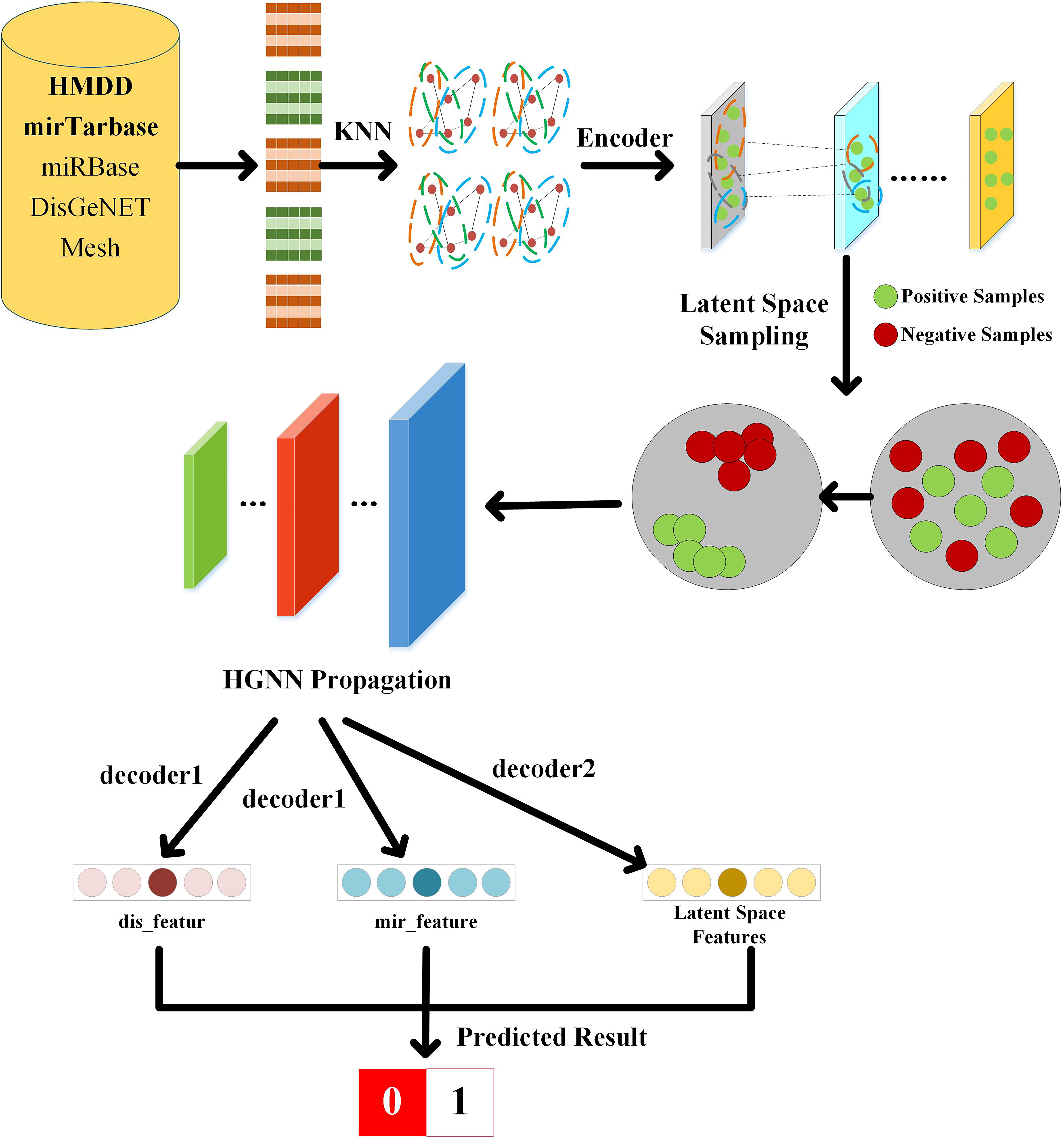
The flow chart of CLHGNNMDA.

2.4.1. Hypergraph construction

The hypergraph in this article is denoted as $G = {V, E, W}$ , V represents the vertex set of the hypergraph, $E$ is the hyperedge set, and $W \in R^{| E | \times | E |}$ represents the diagonal hyperedge weight matrix. Each hyperedge weight $w (e)$ is positive.

Taking miRNA as an example, the miRNA hypermap obtained from the perspective of miRNA and the disease hypermap obtained from the perspective of disease is based on the known association matrix between miRNA and disease.

The constructed miRNA hypergraph is represented as $G_{M} < V_{M}, E_{M}, W_{M} >$ , where $V_{M}$ represents the node set and $E_{M}$ represents the hyperedge set. Treating miRNA or disease instead of miRNA–disease pairs as nodes, the hypergraph nodes constructed from this have different categories. Hypergraph hyperedges are divided into known association hyperedges and similarity hyperedges. To make full use of the known association data between miRNAs and diseases, the miRNAs belonging to the same disease are placed in the same known association hyperedge. Associate similar miRNAs with a similarity higher than a specified similarity threshold to the same similarity hyperedge. The diagonal matrix $W_{M}$ stores the hyperedge weight, and the initial weight of the hyperedge is uniformly set $\frac{1}{| E_{M} |}$ .

The calculation formula of the correlation matrix $H_{M}$ of the miRNA hypergraph $G_{M}$ is as follows. $H_{M} = [A, SSM]$ (5)where A represents a matrix of miRNA expression data.

The calculation formula of SSM is defined as follows: $SSM (i, j) = {\begin{matrix} 1 \begin{matrix} S M (i, j) \geq t \end{matrix} \\ 0 \begin{matrix} otherwise \end{matrix} \end{matrix}$ (6)where t represents a specified similarity threshold.

Similarly, the calculation formula of the correlation matrix $H_{D}$ to construct the disease hypergraph is as follows: $H_{D} = [A^{T}, SSD]$ (7) $SSD (i, j) = {\begin{matrix} 1 \begin{matrix} S D (i, j) \geq t \end{matrix} \\ 0 \begin{matrix} otherwise \end{matrix} \end{matrix}$ (8)

This article uses the KNN strategy to construct multiple hypergraphs. Adjust the similarity threshold and K value as needed to optimize the hypergraph’s performance and interpretability.

2.4.2. Loss function

HGNN utilizes forward propagation to compute outputs and backpropagation to adjust weights and biases, enhancing model expressiveness. The optimization strategy focuses on designing an effective architecture and minimizing the loss function to reduce prediction errors. A composite loss function, integrating KL divergence, contrastive loss, and binary cross-entropy, captures both data structure and attributes, improving model performance.

KL divergence, often used in variational autoencoders, measures the divergence between two probability distributions, such as the encoder’s output and a prior distribution. Minimizing KL divergence ensures continuity and completeness in the latent space, enhancing the diversity of generated data (Yin et al., 2023).

The formula for computing KL divergence loss is as follows: $K L_loss = - \frac{1}{2} \sum_{i = 1}^{N} (1 + \log (σ_{i}^{2}) - μ_{i}^{2} - σ_{i}^{2}$ (9)where N represents the number of nodes or hyperedges. $μ$ is the mean and $σ^{2}$ represents the variance.

Contrastive loss, widely recognized in deep learning and computer vision, improves feature representation by minimizing distances between positive sample pairs and maximizing separations between negative pairs, with this study employing the cosine similarity matrix method with temperature scaling (Long et al., 2024).

In our model, the cosine similarity matrix between two sets of representations is calculated, scaled by a temperature parameter, and used to compute the contrastive loss by summing similarities and averaging the negative log-likelihood, with four sets of contrastive losses combined for the total loss.

Binary cross-entropy loss (Guo et al., 2022), essential for binary classification tasks, measures the difference between predicted probabilities and actual labels, with our model utilizing PyTorch’s binary_cross_entropy_with_logits function to enhance numerical stability and mitigate vanishing gradients.

The overarching loss function in our model is determined as follows: $loss_total = loss 1 + ploss 2 + (1 - p) loss 3$ (10)where $p$ is a weight parameter.

3. RESULTS

3.1. Experimental setting

All experiments were conducted using the Python language, based on the Pytorch deep learning framework. The running machine CPU is Intel(R) Core(TM) i7-4790 CPU @ 3.60 GHz, the memory is 24G, and the GPU is NVIDIA RTX 4070 with 12G memory.

K-fold cross-validation (CV) is especially suitable for limited data scenarios, as noted by Huang et al. (2022c) and has been widely used to evaluate model performance. In our study, we employed fivefold CV repeated 10 times, using the mean results for final evaluation. Performance was assessed using receiver operating characteristic (ROC) curves and area under the ROC curve (AUC) as the primary indicators, with additional metrics including accuracy, precision, recall, F1-score, and area under the precision-recall curve (AUPR) (Sokolova and Lapalme, 2009).

The formulas used to calculate the evaluation metrics in this experiment are provided below. $\begin{array}{c} Precision = \frac{T P}{T P + F P}, recall = \frac{T P}{T P + F N}, F 1 - socre = \frac{2 T P}{2 T P + F N + F P}, \\ A ccuracy = \frac{T P + T N}{TP + TN + FP + FN}, MCC = \frac{T P \times T N - F P \times F N}{\sqrt{(T P + F P) (T P + F n) (T N + F P) (T N + F N)}} \end{array}$ (11)where TP stands for true-positive cases, TN stands for true-negative cases, FP refers to false-positive cases, and FN signifies false-negative cases.

Preliminary hyperparameter values for the CLHGNNMDA model were determined based on prior research insights, followed by the execution of a fivefold CV on the CLHGNNMDA model. Table 1 provides the initial experimental settings for the key hyperparameters used in the CLHGNNMDA model.

Table 1.

Main Hyperparameters of CLHGNNMDA Model

Hyperparameters	Parameter value
lr	0.002
p	0.7
k	10
weight_decay	0.0005
temperature	0.7

In Table 1, “lr” indicates the learning rate, which controls the magnitude of parameter updates, while “weight_decay” serves as the coefficient for L2 regularization, designed to reduce overfitting by discouraging large parameter values. The parameter “p” modulates the relative contributions of the three loss functions in predicting miRNA–disease associations, and “k” defines the number of neighboring points considered in hypergraph construction, influencing both the sparsity and effectiveness of the algorithm. The “Temperature” parameter, typically ranging from 0.1 to 1, plays a key role in the computation of contrastive loss by shaping learning dynamics and overall model performance. Identifying the optimal value for this parameter often requires empirical experimentation through multiple iterations of testing and fine-tuning, as it can significantly affect model accuracy.

A fivefold CV experiment was performed on the CLHGNNMDA model using the HMDD v3.2 database, with hyperparameters specified in Table 1. The experimental results are depicted in Figure 2, where Figure 2a illustrates the accuracy line graph, and Figure 2b shows the corresponding ROC curve.

FIG. 2.

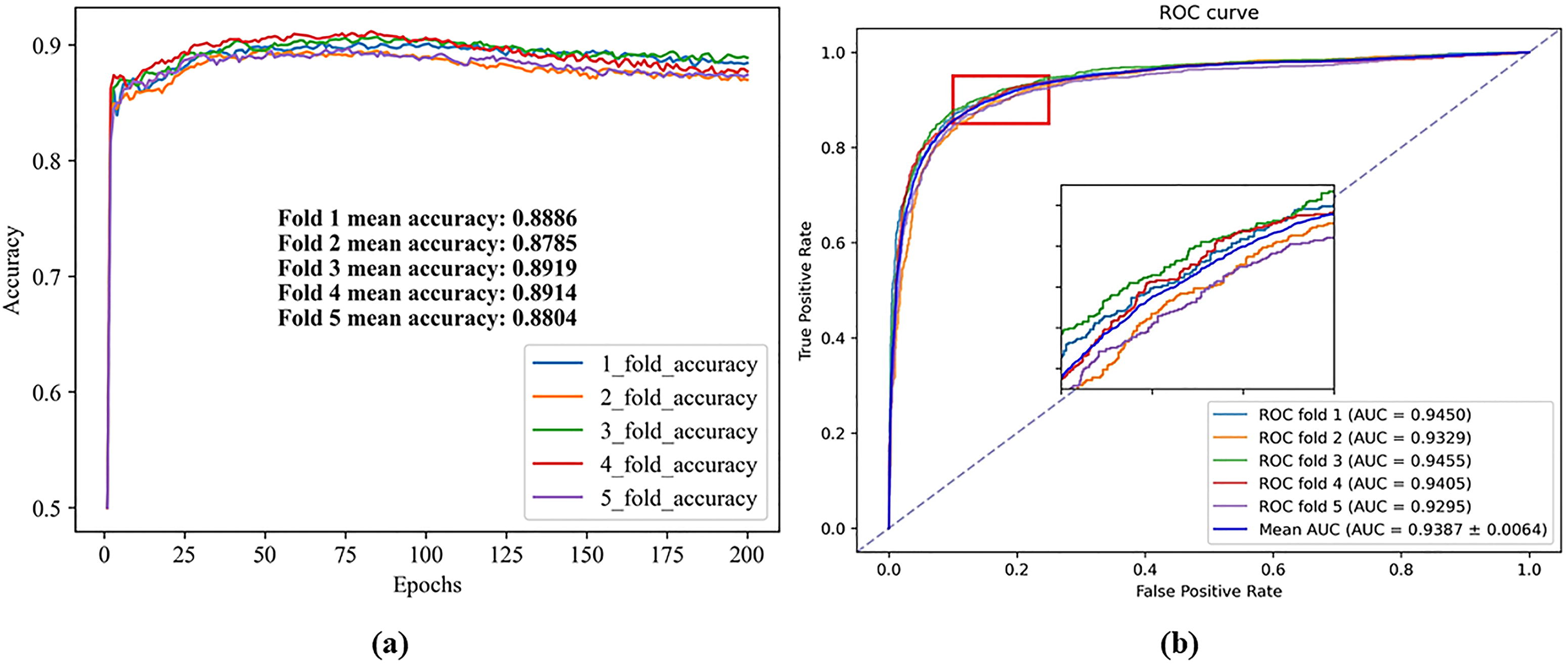
Initial experimental results.

As shown in Figure 2, the CLHGNNMDA model achieves an average AUC of 0.9387. Through iterative training, the model learns patterns and features, with each epoch refining the model’s parameters to minimize the loss function. Determining the optimal number of epochs requires experimentation, often combined with early stopping to avoid overfitting. In this study, 200 epochs were established as optimal for the CLHGNNMDA model through extensive testing. Dropout regularization, which randomly omits neurons during training, enhances model robustness by preventing reliance on specific neurons. We use a dropout rate of 0.5, in line with common practice in the literature.

3.2. Optuna framework optimizes hyperparameters

This section uses the Optuna hyperparameter automated tuning framework to optimize the five hyperparameters of lr, weight_decay, k, p, and temperature in the CLHGNNMDA model. Optuna is an advanced framework designed for the automated tuning of hyperparameters, compatible with a plethora of machine-learning libraries. Utilizing Optuna facilitates the expedient identification of the optimal hyperparameter combination, thereby augmenting model efficacy.

Initially, the hyperparameter search space within the Optuna framework is defined, as delineated in Table 2.

Table 2.
Optuna Hyperparameter Tuning Search Range

Hyperparameter Parameter value range Parameter type

lr [1e-4, 1e-3] Float

weight_decay [1e-4, 1e-1] Float

p [0.1, 0.2, 0.3, 0.4, 0.5, 0.6, 0.7, 0.8, 0.9] Float

k [5, 6, 7, 8, 9, 10, 11, 12, 13, 14, 15, 16, 17, 18, 19, 20] Int

temperature [0.5, 0.6, 0.7, 0.8, 0.9] Float

Hyperparameter	Parameter value range	Parameter type
lr	[1e-4, 1e-3]	Float
weight_decay	[1e-4, 1e-1]	Float
p	[0.1, 0.2, 0.3, 0.4, 0.5, 0.6, 0.7, 0.8, 0.9]	Float
k	[5, 6, 7, 8, 9, 10, 11, 12, 13, 14, 15, 16, 17, 18, 19, 20]	Int
temperature	[0.5, 0.6, 0.7, 0.8, 0.9]	Float

Based on the hyperparameter search range outlined in Table 2, we employed Optuna’s median pruning decision tree algorithm to conduct 100 hyperparameter searches. This optimization process yielded a maximum AUC value of 0.9635, with the results illustrated in Figure 3. The optimal parameters identified through Optuna’s hyperparameter optimization framework are listed in Table 3.

FIG. 3.

Hyperparameter optimization using the Optuna framework. (a) High-dimensional parameter relationship diagram, (b) parameter importance comparison, (c) hyperparameter search history, and (d) ROC curves post-optimization with Optuna. AUC, area under the curve.

Table 3.

The Optimal Value of Optuna Search for the Main Hyperparameters of CLHGNNMDA

Hyperparameters	Optimal parameter values
lr	0.0009
p	0.1
k	15
weight_decay	0.004
temperature	0.9

Slight variations in results may occur across different executions when using the Optuna framework for hyperparameter tuning. Therefore, in the experiment, this procedure was iterated 10 times, with the results presented in Table 3 representing the tuning outcome that achieved the highest AUC value among the 10 experimental iterations.

As illustrated in Figure 3d, the application of the Optuna framework for hyperparameter optimization elevated the experimental average AUC of the CLHGNNMDA model to 0.9635, marking an improvement of approximately 2.33% over the pretuning performance. This enhancement underscores the efficacy of the Optuna hyperparameter optimization framework in identifying an optimal set of hyperparameters, thereby significantly augmenting the performance of the CLHGNNMDA model.

3.3. Parameter analysis

In the previous experimental phase, broad value ranges were initially set for the hyperparameters lr and weight decay, based on prior research. This section focuses on refining these ranges by narrowing them, guided by the optimal values identified earlier, to better examine their effects on model performance.

For lr, Optuna’s optimization determined 0.0009 as the best value. Thus, experiments were conducted over the range (0.0005, 0.0006, 0.0007, 0.0008, 0.0009, 0.001, 0.002, 0.003, 0.004, 0.005). As shown in Figures 4a and 4b, the value lr = 0.0009 yielded the highest AUC (0.9634) and AUPR (0.9646), validating Optuna’s prior results. Consequently, lr = 0.0009 was chosen for further testing.

FIG. 4.

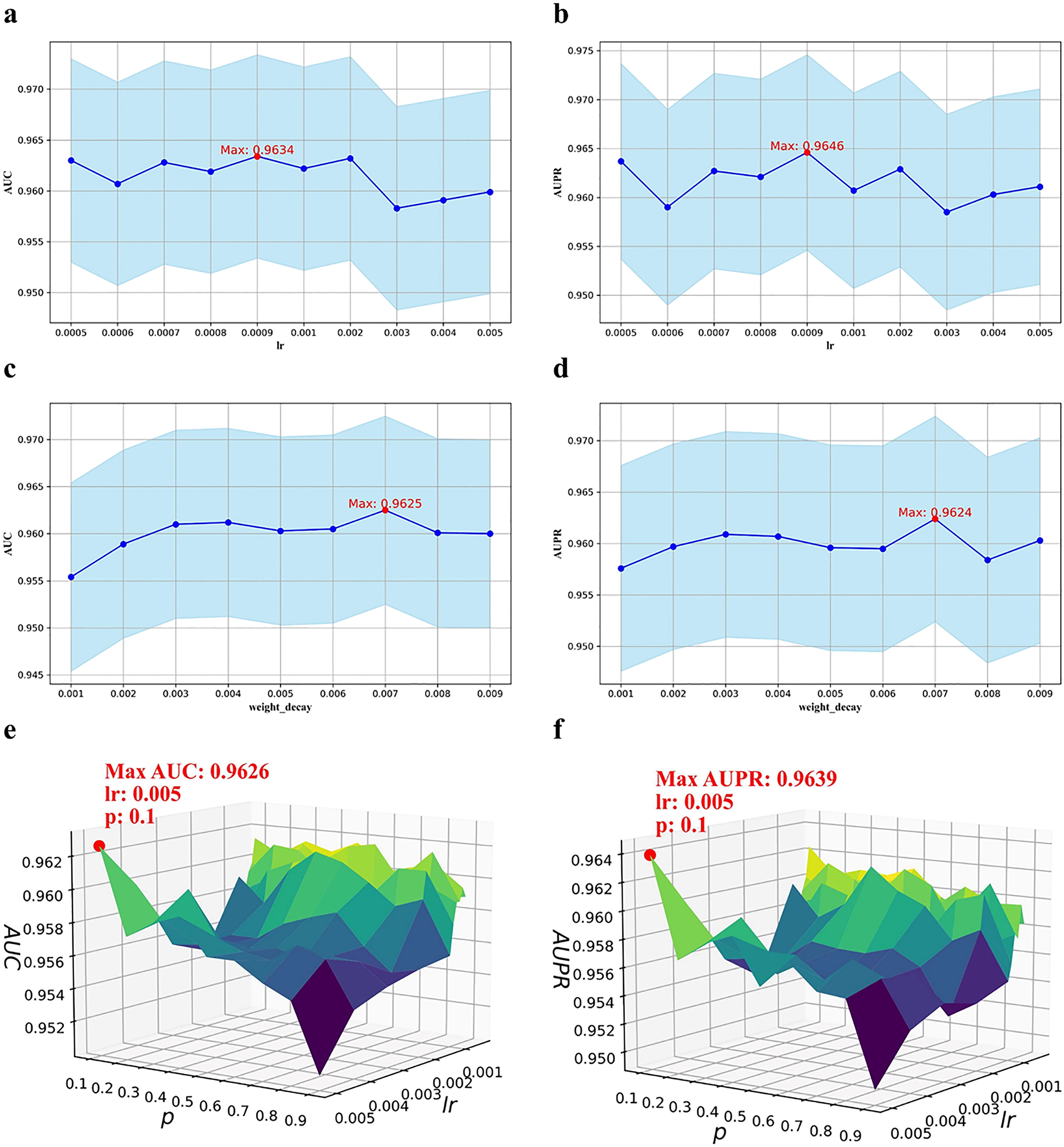
Parameter analysis. Building on previous experimental results, we further refined the hyperparameter ranges for learning rate (lr) and weight decay, conducting extensive experiments to identify the optimal settings. Panels (a) and (b) present the results of lr optimization within this narrowed range, while (c) and (d) illustrate the analysis of weight decay over its refined range. Panels (e) and (f) demonstrate the combined effects of lr and dropout rate (p) on model performance.

Similarly, based on the weight decay value of 0.004 suggested by Optuna, the range (0.001 to 0.009) was explored. Figures 4c and 4d demonstrate that weight decay = 0.007 provided the best AUC (0.9625) and AUPR (0.9624), though slightly different from the previous value. After averaging results from 10 additional trials, weight decay = 0.005 was selected for future use.

Additionally, the joint effects of lr and p on model performance were examined. Figures 4e and 4f reveal that the combination of lr = 0.005 and p = 0.1 produced the optimal AUC (0.9626) and AUPR (0.9639). After extensive experimentation, the final settings chosen for subsequent studies were lr = 0.0009 and p = 0.1.

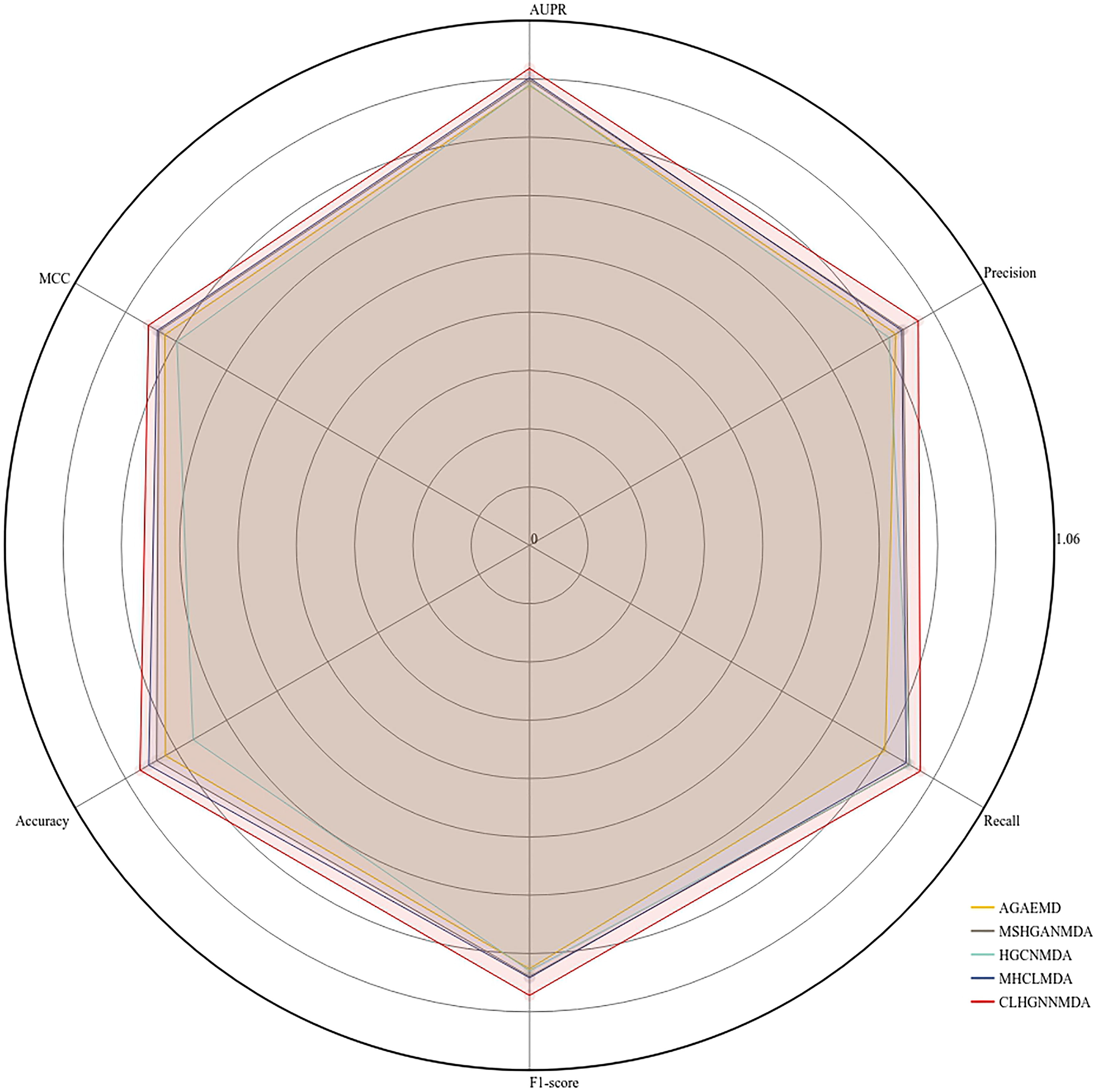
3.4. Performance comparison with other methods

This section presents an evaluation of the CLHGNNMDA model’s performance through a comparative analysis with four established computational techniques. The assessment utilizes fivefold CV on the HMDD v3.2 database. The methods considered in this analysis include MHCLMDA (Peng et al., 2023c), HGCNMDA (Peng et al., 2023b), MSHGANMDA (Wang et al., 2023b), and AGAEMD (Zhang et al., 2023). The methods we have selected are widely recognized and extensively validated as effective within our field, making them highly representative. Table 4 presents the evaluation metrics for the various methods, while Figure 5 depicts the ROC curves generated from the fivefold CV of these methods. The hyperparameter configurations for the various experimental methods are presented in Table 5.

FIG. 5.

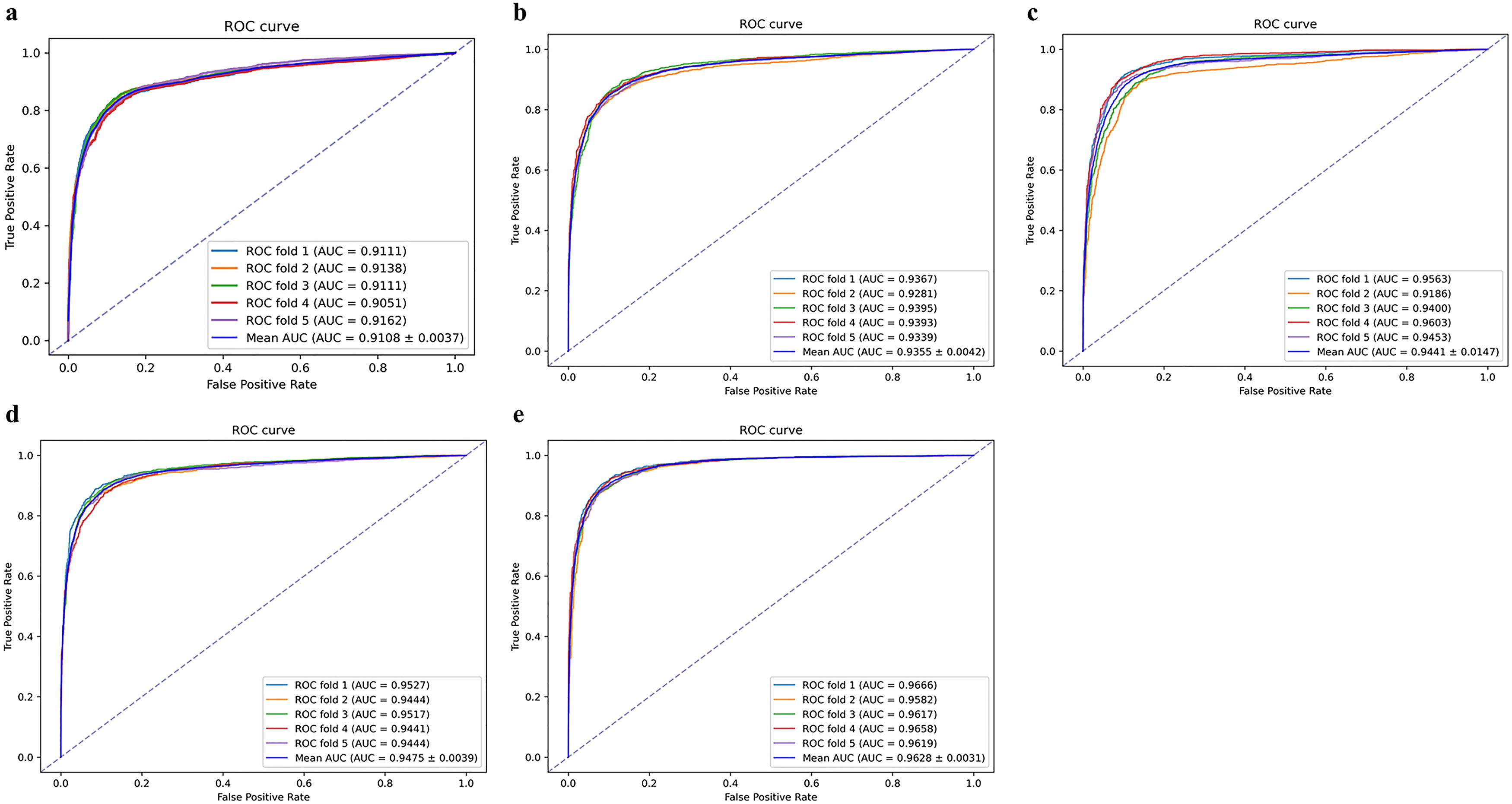
ROC curves for fivefold cross-validation of various models. This figure compares the performance of the CLHGNNMDA model with four established computational methods using fivefold cross-validation on the HMDD v3.2 database. The methods evaluated include (a) AGAEMD, (b) MSHGANMDA, (c) HGCNMDA, (d) MHCLMDA, and (e) CLHGNNMDA. HGCNMDA, heterogeneous graph convolutional network.

Table 4.

Comparison of Prediction Results of Various Models

Methods	AUPR	Precision	Recall	F1-score	Accuracy	MCC
AGAEMD	0.9213	0.8667	0.8308	0.8484	0.8515	0.8722
MSHGANMDA	0.9301	0.8630	0.8620	0.8619	0.8620	0.7161
HGCNMDA	0.9155	0.8126	0.8869	0.8102	0.7712	0.8052
MHCLMDA	0.9400	0.8768	0.8637	0.7996	0.7996	0.8096
CLHGNNMDA	0.9656	0.9139	0.9060	0.9098	0.9099	0.8203

Table 5.

Hyperparameter Settings of Various Models

Hyperparameters	CLHGNNMDA	AGAEMD	MSHGANMDA	HGCNMDA	MHCLMDA
epochs	200	200	200	200	200
lr	0.0009	0.0009	0.0009	0.0009	0.0009
weight_decay	0.004	0.004	0.004	0.004	0.004
dropout	0.5	—	0.3	—	0.5
alpha	—	—	—	0.4	0.7
λ	—	—	—	—	0.6
p	0.1	—	—	—	—
k	15	—	—	—	10
temperature	0.9	—	—	—	—
attn_heads	—	—	4	—	—
attn_size	—	—	128	—	—
hidden	—	4	—	—	128
heads_per_layer	—	6	—	—	—
embedding_features	—	200	—	—	—

To compare different methods in pairs, the Wilcoxon signed rank test was utilized, and the results are presented in Table 6. This test is a nonparametric statistical tool commonly used for paired data, particularly advantageous when dealing with small sample sizes or data that deviate from normality. In this study, comparisons with p-values below 0.05 indicate statistically significant differences between two algorithms, while p-values above 0.05 suggest no significant difference.

Table 6.

Results of Wilcoxon Signed-Rank Test

Comparison	p-Value
AGAEMD vs MSHGANMDA	0.5625
AGAEMD vs HGCNMDA	0.21875
AGAEMD vs MHCLMDA	0.4375
AGAEMD vs CLHGNNMDA	0.15625
MSHGANMDA vs HGCNMDA	0.5625
MSHGANMDA vs MHCLMDA	0.84375
MSHGANMDA vs CLHGNNMDA	0.03125
HGCNMDA vs MHCLMDA	0.3125
HGCNMDA vs CLHGNNMDA	0.03125
MHCLMDA vs CLHGNNMDA	0.03125

According to Table 6, CLHGNNMDA emerges as the best-performing algorithm. It exhibits statistically significant differences when compared with MSHGANMDA, HGCNMDA, and MHCLMDA, all with p-values under 0.05, suggesting its superior performance across multiple evaluation metrics. Although there was no significant difference ( p-value > 0.05) between CLHGNNMDA and AGAEMD, AGAEMD did not show any substantial disadvantage in comparison to other algorithms. Moreover, no significant differences ( p > 0.05) were observed between MSHGANMDA, MHCLMDA, and HGCNMDA.

In conclusion, the Wilcoxon signed rank test results demonstrate that CLHGNNMDA performs significantly better than most other algorithms, particularly when compared with MSHGANMDA, HGCNMDA, and MHCLMDA. While no significant difference was detected between CLHGNNMDA and AGAEMD, CLHGNNMDA still showcases superior performance across various evaluation metrics.

3.5. Other databases experiment

To further evaluate the performance of the CLHGNNMDA model, we carried out additional validation experiments using the HMDD v2.0 dataset (Li et al., 2014). We utilized this dataset to conduct a fivefold CV on the models listed in Table 4, while keeping the hyperparameters consistent with those outlined in Table 3. The results of these experiments are presented in Figure 6.

FIG. 6.

Experimental results on HMDD v2.0 database. This figure compares the performance of the CLHGNNMDA model with four established computational methods using fivefold cross-validation on the HMDD v2.0 database.

As illustrated in Figure 6, the CLHGNNMDA model achieves the best performance across all the evaluated indicators compared to the other models.

3.6. Ablation experiments

To substantiate the CLHGNNMDA model’s effectiveness further, ablation studies were executed. These involved comparative analyses between the CLHGNNMDA model and a variant, CLHGNNMDA_1, from which the contrastive loss component was excised.

The comparative outcomes, as depicted in Figure 7, reveal a notable enhancement in model performance subsequent to the incorporation of the contrastive loss function.

FIG. 7.

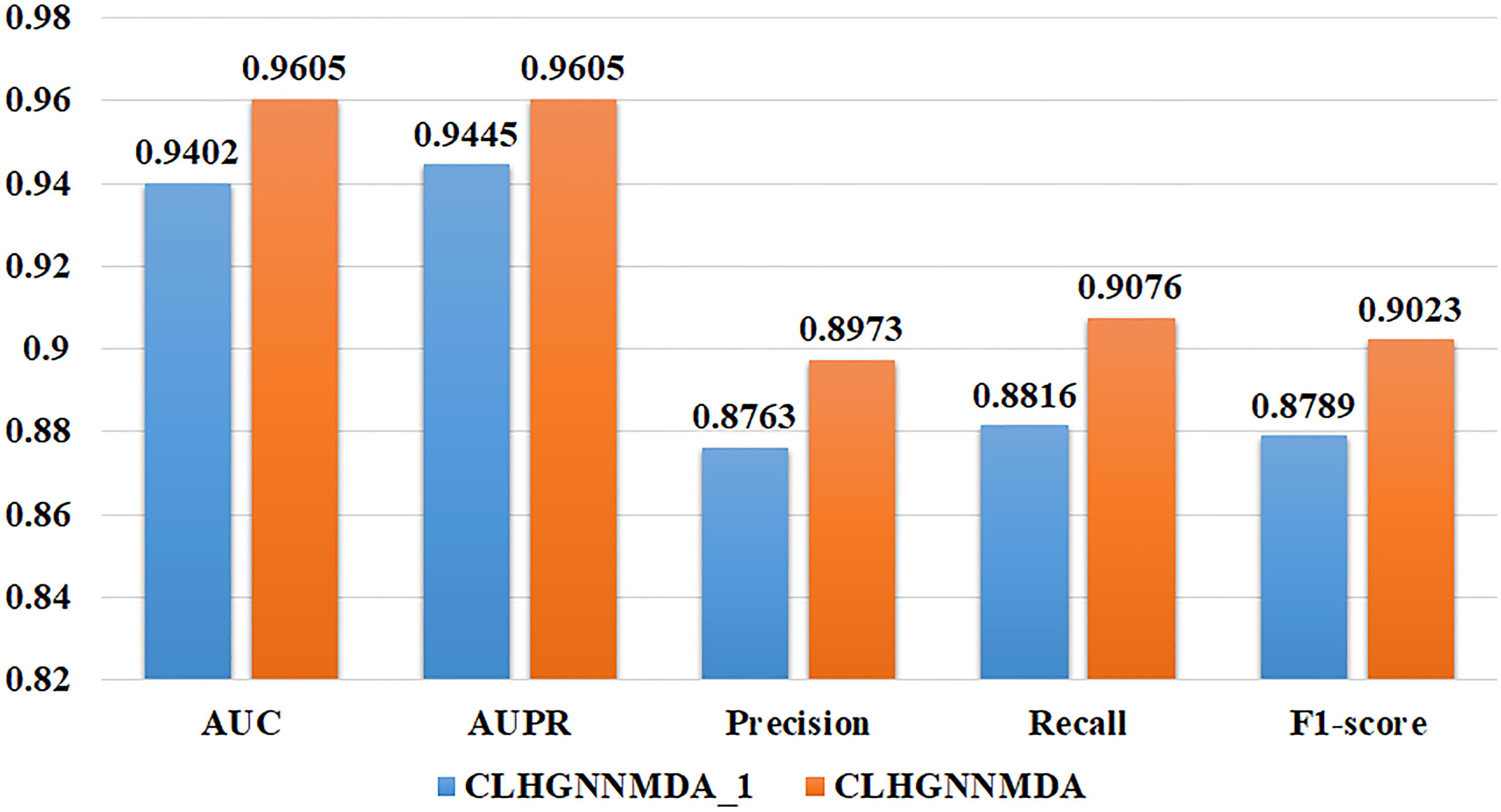
Comparative analysis of performance outcomes from ablation experiments.

Further investigations were carried out by eliminating the KL divergence loss function, maintaining solely the binary cross-entropy loss function. The outcomes of these experiments were significantly inferior, thereby not warranting inclusion herein.

3.7. Case studies

To corroborate the predictive accuracy of the CLHGNNMDA model further, this section conducts a case study on breast tumors. Employing the trained CLHGNNMDA model, the study predicts the top 10 candidate miRNA–disease pairs for breast tumors. These candidates were then scrutinized against the miRNA–disease association database dbDEMC (Yang et al., 2010) to validate the existence and biological experimentally confirmed associations of these candidate miRNAs with the specified diseases.

An inquiry into dbDEMC for the top 10 predicted candidate miRNAs associated with breast tumors, as identified by the CLHGNNMDA model, yielded retrievable results for all candidates. Subsequent analysis conducted on the dbDEMC analysis page (https://www.biosino.org/dbDEMC/metaProfiling/detail) furnished a Meta-profiling Heatmap, as exhibited in Figure 8.

FIG. 8.

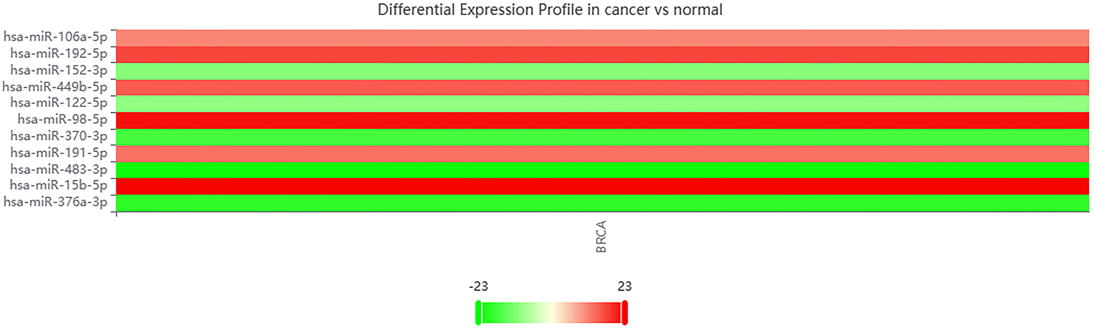
Meta-profiling heatmap in dbDEMC. To validate the predictive accuracy of the CLHGNNMDA model, a case study on breast tumors was conducted. The model identified the top 10 candidate miRNA–disease pairs for breast tumors. This figure presents the resulting meta-profiling heatmap from the dbDEMC analysis page (https://www.biosino.org/dbDEMC/metaProfiling/detail).

The findings from this case study affirm the CLHGNNMDA model’s effectiveness and its commendable predictive prowess.

4. DISCUSSION

miRNAs are crucial in various biological processes and are linked to the development of numerous diseases. Investigating miRNA–disease interactions is vital for advancing the prevention, diagnosis, and treatment of complex diseases. With the rise of computational technologies, deep learning has become a valuable tool for efficiently identifying disease-associated miRNAs due to its strong modeling and feature extraction capabilities. This study introduces a novel model, CLHGNNMDA, which integrates contrastive learning within a HGNN framework to predict miRNA–disease associations. The contrastive learning strategy enhances feature representation, generalization, and model interpretability while addressing overfitting and data imbalance issues.

The CLHGNNMDA model’s effectiveness is validated through fivefold CV, achieving an average AUC of 0.9635 and an AUPR of 0.9656, outperforming existing methods. Additionally, a case study on breast tumor-associated miRNAs confirms the top 10 predictions using existing research. Despite its strong performance, there is room for improvement, particularly in incorporating more diverse biological data and integrating heterogeneous information to further enhance predictive accuracy.

5. CONCLUSION

This research introduces a novel HGNN model, designated CLHGNNMDA, which is enhanced through contrastive learning to forecast miRNA–disease associations. The distinguishing feature of the CLHGNNMDA model resides in its innovative construction of multiple hypergraphs coupled with the integration of contrastive learning techniques. The strong experimental results of the CLHGNNMDA model highlight its potential as an influential tool for advancing miRNA–disease association research, offering valuable insights and practical applications in this domain. The future of miRNA–disease association prediction will likely emphasize the integration of diverse omics datasets, the application of advanced machine learning, and the need for greater model interpretability. By synthesizing data from various biological sources, these predictive models will become increasingly accurate, uncovering new relationships between miRNAs and diseases. The use of cutting-edge algorithms, such as deep learning, will enhance the ability to model complex biological interactions, even in the presence of data imbalances. Ensuring that these models are transparent and interpretable will be crucial for their application in clinical settings. Additionally, collaboration and data sharing will be essential in building robust datasets, refining predictions, and advancing personalized medicine.

Footnotes

AUTHORS’ CONTRIBUTIONS

R.Z. and Y.W.: Conceptualization and methodology. Y.W.: Data curation. R.Z.: Writing. L.Y.D. and Y.W.: Review and editing. All authors have read and agreed to the published version of the article.

DATA AVAILABILITY STATEMENT

The source code and data can be obtained from .

AUTHOR DISCLOSURE STATEMENT

The authors declare no conflict of interest.

FUNDING INFORMATION

This work was supported in part by Shandong Social Science Planning Fund Program No. 21BTQJ02 and the National Natural Science Foundation of China under Grant No. 62472250.

References

Barut

, Akdeniz

, Isbir

. Investigation of miRNA-223-3p expression in non-small cell lung cancers. Anticancer Res, 2024; 44(2):585–591; doi: 10.21873/anticanres.16847

Bozzarelli

, Orsini

, Isidori

, et al. miRNA-221 and miRNA-483-3p dysregulation in esophageal adenocarcinoma. Cancers (Basel), 2024; 16(3):1–16; doi: 10.3390/cancers16030591

Chen

, Huang

, Xie

, et al. EGBMMDA: Extreme gradient boosting machine for miRNA-disease association prediction. Cell Death Dis, 2018a;9(1):3–16; doi: 10.1038/s41419-017-0003-x

Chen

, Niu

Y-W

, Wang

G-H

, et al. HAMDA: Hybrid approach for miRNA-disease association prediction. J Biomed Inform, 2017; 76:50–58; doi: 10.1016/j.jbi.2017.10.014

Chen

, Xie

, Wang

, et al. BNPMDA: Bipartite network projection for miRNA-disease association prediction. Bioinformatics, 2018b;34(18):3178–3186; doi: 10.1093/bioinformatics/bty333

Chen

, Xie

, Zhao

, et al. MicroRNAs and complex diseases: From experimental results to computational models. Brief Bioinform, 2019; 20(2):515–539; doi: 10.1093/bib/bbx130

Feng

, You

, Zhang

, et al. Hypergraph neural networks. In: Proceedings of the AAAI Conference on Artificial Intelligence. 2019, pp.3558–3565.

Gao

, Zhang

, Lin

, et al. Hypergraph learning: Methods and practices. IEEE Trans Pattern Anal Mach Intell, 2022; 44(5):2548–2566; doi: 10.1109/tpami.2020.3039374

Guo

, Chen

, et al. Multi-stage attentive network for motion deblurring via binary cross-entropy loss. Entropy (Basel), 2022; 24(10); doi: 10.3390/e24101414

10.

, Fan

, Wu

, et al. Momentum contrast for unsupervised visual representation learning. In: Proceedings of the IEEE/CVF conference on computer vision and pattern recognition. 2020, pp.9729–9738.

11.

Huang

, Zhang

, Chen

. Updated review of advances in microRNAs and complex diseases: Experimental results, databases, webservers and data fusion. Brief Bioinform, 2022a;23(6):1–20; doi: 10.1093/bib/bbac397

12.

Huang

, Zhang

, Chen

. Updated review of advances in microRNAs and complex diseases: Taxonomy, trends and challenges of computational models. Brief Bioinform, 2022b;23(5):1–32; doi: 10.1093/bib/bbac358

13.

Huang

, Zhang

, Chen

. Updated review of advances in microRNAs and complex diseases: Towards systematic evaluation of computational models. Brief Bioinform, 2022c;23(6):1–15; doi: 10.1093/bib/bbac407

14.

Huang

, Shi

, Gao

, et al. HMDD v3.0: A database for experimentally supported human microRNA-disease associations. Nucleic Acids Res, 2019; 47(D1):D1013–D1017; doi: 10.1093/nar/gky1010

15.

Jiang

, Wei

, Feng

, et al. Dynamic hypergraph neural networks. In: Proceedings of the Twenty-Eighth International Joint Conference on Artificial Intelligence (IJCAI-19). 2019, pp.2635–2641.

16.

Jiang

, Wang

, Hao

, et al. miR2Disease: A manually curated database for microRNA deregulation in human disease. Nucleic Acids Research, 2009; 37(Database issue):D98–D104; doi: 10.1093/nar/gkn714

17.

Kozomara

, Birgaoanu

, Griffiths-Jones

. miRBase: From microRNA sequences to function. Nucleic Acids Res, 2019; 47(D1):D155–D162; doi: 10.1093/nar/gky1141

18.

Lan

, Dong

, Chen

, et al. IGNSCDA: Predicting CircRNA-disease associations based on improved graph convolutional network and negative sampling. IEEE/ACM Trans Comput Biol Bioinform, 2022a;19(6):3530–3538; doi: 10.1109/tcbb.2021.3111607

19.

Lan

, Dong

, Zhang

, et al. Benchmarking of computational methods for predicting circRNA-disease associations. Brief Bioinform, 2023; 24(1):1–22; doi: 10.1093/bib/bbac613

20.

Lan

, Lai

, Chen

, et al. LDICDL: LncRNA-disease association identification based on collaborative deep learning. IEEE/ACM Trans Comput Biol Bioinform, 2022b;19(3):1715–1723; doi: 10.1109/tcbb.2020.3034910

21.

Lan

, Li

, Chen

, et al. LGCDA: Predicting CircRNA-disease association based on fusion of local and global features. IEEE/ACM Trans Comput Biol Bioinform, 2024; 21(5):1413–1422; doi: 10.1109/tcbb.2024.3387913

22.

Lan

, Wang

, Li

, et al. Predicting microRNA-disease associations based on improved microRNA and disease similarities. IEEE ACM Trans Comput Biol Bioinform, 2018; 15(6):1774–1782; doi: 10.1109/tcbb.2016.2586190

23.

, Liu

, Hu

, et al. A novel computational model for predicting microRNA-disease associations based on heterogeneous graph convolutional networks. Cells, 2019; 8(9):1–17; doi: 10.3390/cells8090977

24.

, Wang

, Zhong

, et al. Circulating small extracellular vesicle-based miRNA classifier for follicular thyroid carcinoma: A diagnostic study. Br J Cancer, 2024; 130(6):925–933; doi: 10.1038/s41416-024-02575-0

25.

, Liu

, Zhang

, et al. PmDNE: Prediction of miRNA-disease association based on network embedding and network similarity analysis. Biomed Res Int, 2020; 2020:6248686–6248689; doi: 10.1155/2020/6248686

26.

, Gao

, Zheng

C-H

, et al. SNFIMCMDA: Similarity network fusion and inductive matrix completion for miRNA-disease association prediction. Front Cell Dev Biol, 2021; 9:617569–617510; doi: 10.3389/fcell.2021.617569

27.

, Qiu

, Tu

, et al. HMDD v2.0: A database for experimentally supported human microRNA and disease associations. Nucleic Acids Res, 2014; 42(Database issue):D1070–D1074; doi: 10.1093/nar/gkt1023

28.

Liang

, Liu

, Song

, et al. HMCDA: A novel method based on the heterogeneous graph neural network and metapath for circRNA-disease associations prediction. BMC Bioinformatics, 2023; 24(1):335–313; doi: 10.1186/s12859-023-05441-7

29.

Liu

, Huang

, Nie

, et al. SMALF: miRNA-disease associations prediction based on stacked autoencoder and XGBoost. BMC Bioinformatics, 2021; 22(1):219–218; doi: 10.1186/s12859-021-04135-2

30.

Liu

, Ren

, Chen

, et al. Predicting lncRNA-miRNA interactions based on logistic matrix factorization with neighborhood regularized. Knowledge Based Syst, 2020; 191:105261–105267; doi: 10.1016/j.knosys.2019.105261

31.

Liu

, Kuang

, Deng

. GCNPCA: miRNA-disease associations prediction algorithm based on graph convolutional neural networks. IEEE ACM Trans Comput Biol Bioinform, 2023; 20(2):1041–1052; doi: 10.1109/tcbb.2022.3203564

32.

Liu

, Wei

, Zhang

, et al. SSCRB: Predicting circRNA-RBP interaction sites using a sequence and structural feature-based attention model. IEEE J Biomed Health Inform, 2024; 28(3):1762–1772; doi: 10.1109/jbhi.2024.3354121

33.

Liu

, Zhang

, Yap

P-T

, et al. View-aligned hypergraph learning for Alzheimer’s disease diagnosis with incomplete multi-modality data. Med Image Anal, 2017; 36:123–134; doi: 10.1016/j.media.2016.11.002

34.

Long

, Du

, Li

. Two momentum contrast in triplet for unsupervised visual representation learning. Multimed Tools Appl, 2024; 83(4):10467–10480; doi: 10.1007/s11042-023-15998-3

35.

Mastropietro

, De Carlo

, Anagnostopoulos

. XGDAG: Explainable gene-disease associations via graph neural networks. Bioinformatics, 2023; 39(8):1–9; doi: 10.1093/bioinformatics/btad482

36.

Nguyen

, Mamitsuka

. Learning on hypergraphs with sparsity. IEEE Trans Pattern Anal Mach Intell, 2021; 43(8):2710–2722; doi: 10.1109/tpami.2020.2974746

37.

Pan

, Li

, Che

, et al. Low-rank tensor regularized graph fuzzy learning for multi-view data processing. IEEE Trans Consumer Electron, 2024; 70(1):2925–2938; doi: 10.1109/tce.2023.3301067

38.

Pantaleao

, Loche

, Fernandez-Twinn

, et al. Programming of cardiac metabolism by miR-15b-5p, a miRNA released in cardiac extracellular vesicles following ischemia-reperfusion injury. Mol Metab, 2024; 80:101875–101875; doi: 10.1016/j.molmet.2024.101875

39.

Peng

, Huang

, Tian

, et al. Predicting potential microbe-disease associations with graph attention autoencoder, positive-unlabeled learning, and deep neural network. Front Microbiol, 2023a;14:1244527–1244515; doi: 10.3389/fmicb.2023.1244527

40.

Peng

, Che

, Dai

, et al. Predicting miRNA-disease associations from miRNA-gene-disease heterogeneous network with multi-relational graph convolutional network model. IEEE/ACM Trans Comput Biol Bioinform, 2023b;20(6):3363–3375; doi: 10.1109/tcbb.2022.3187739

41.

Peng

, He

, Dai

, et al. MHCLMDA: Multihypergraph contrastive learning for miRNA-disease association prediction. Brief Bioinform, 2023c;25(1):1–12; doi: 10.1093/bib/bbad524

42.

Pinero

, Manuel Ramirez-Anguita

, Sauch-Pitarch

, et al. The DisGeNet knowledge platform for disease genomics: 2019 update. Nucleic Acids Research, 2020; 48(D1):D845–D855; doi: 10.1093/nar/gkz1021

43.

Pinero

, Sauch

, Sanz

, et al. The DisGeNET cytoscape app: Exploring and visualizing disease genomics data. Comput Struct Biotechnol J, 2021; 19:2960–2967; doi: 10.1016/j.csbj.2021.05.015

44.

, Chen

, Yin

, et al. Prediction of potential miRNA-disease associations using matrix decomposition and label propagation. Knowledge Based Syst, 2019; 186:104963–104910; doi: 10.1016/j.knosys.2019.104963

45.

Sheng

, Xie

, Wang

, et al. A survey of deep learning for detecting miRNA-disease associations: Databases, computational methods, challenges, and future directions. IEEE ACM Trans Comput Biol Bioinform, 2024; 21(3):328–347; doi: 10.1109/tcbb.2024.3351752

46.

Shi

, Zhang

, Zhan

, et al. Hypergraph-induced convolutional networks for visual classification. IEEE Trans Neural Netw Learn Syst, 2019; 30(10):2963–2972; doi: 10.1109/tnnls.2018.2869747

47.

Sokolova

, Lapalme

. A systematic analysis of performance measures for classification tasks. Inf Process Manag, 2009; 45(4):427–437; doi: 10.1016/j.ipm.2009.03.002

48.

Sujamol

, Vimina

, Krishnakumar

. Improving miRNA disease association prediction accuracy using integrated similarity information and deep autoencoders. IEEE ACM Trans Comput Biol Bioinform, 2023; 20(2):1125–1136; doi: 10.1109/tcbb.2022.3195514

49.

Sun

, Li

, Feng

, et al. NTSMDA: Prediction of miRNA-disease associations by integrating network topological similarity. Mol Biosyst, 2016; 12(7):2224–2232; doi: 10.1039/c6mb00049e

50.

Sun

, Sun

, Zhao

. A deep learning method for predicting metabolite-disease associations via graph neural network. Brief Bioinform, 2022; 23(4):1–11; doi: 10.1093/bib/bbac266

51.

Tang

, Luo

, Shen

, et al. Multi-view multichannel attention graph convolutional network for miRNA-disease association prediction. Brief Bioinform, 2021; 22(6):1–12; doi: 10.1093/bib/bbab174

52.

Wang

, Li

, Yue

, et al. NMCMDA: Neural multicategory MiRNA-disease association prediction. Brief Bioinform, 2021; 22(5):1–11; doi: 10.1093/bib/bbab074

53.

Wang

, Xu

, Tian

, et al. MDAlmc: A novel low-rank matrix completion model for miRNA-disease association prediction by integrating similarities among miRNAs and diseases. Curr Gene Ther, 2023a;23(4):316–327; doi: 10.2174/1566523223666230419101405

54.

Wang

, Yan

, Yang

. Neural graph matching network: Learning Lawler’s quadratic assignment problem with extension to hypergraph and multiple-graph matching. IEEE Trans Pattern Anal Mach Intell, 2022a;44(9):5261–5279; doi: 10.1109/tpami.2021.3078053

55.

Wang

, Wang

, Qiao

, et al. MSHGANMDA: Meta-subgraphs heterogeneous graph attention network for miRNA-disease association prediction. IEEE J Biomed Health Inform, 2023b;27(10):4639–4648; doi: 10.1109/jbhi.2022.3186534

56.

Wang

, Zhang

, Sun

, et al. Predicting the potential human lncRNA-miRNA interactions based on graph convolution network with conditional random field. Brief Bioinform, 2022b;23(6):1–9; doi: 10.1093/bib/bbac463

57.

Wang

, Song

, Wei

, et al. Predicting potential drug-disease associations based on hypergraph learning with subgraph matching. Interdiscip Sci, 2023c;15(2):249–261; doi: 10.1007/s12539-023-00556-0

58.

, Zhu

, Wang

, et al. An ensemble learning framework for potential miRNA-disease association prediction with positive-unlabeled data. Comput Biol Chem, 2021; 95:107566–107513; doi: 10.1016/j.compbiolchem.2021.107566

59.

Yadati

, Nimishakavi

, Yadav

, et al. Hypergcn: A new method for training graph convolutional networks on hypergraphs. Adv Neural Inform Process Syst, 2019; 32:1–12.

60.

Yang

, Sun

, Jin

, et al. Multi-task aquatic toxicity prediction model based on multi-level features fusion. J Adv Res, 2024; 1–13; doi: 10.1016/j.jare.2024.06.002

61.

Yang

, Ren

, Liu

, et al. dbDEMC: A database of differentially expressed miRNAs in human cancers. BMC Genomics, 2010; 11(Suppl 4):S5–S8; doi: 10.1186/1471-2164-11-s4-s5

62.

Yin

, Zhu

, Wu

, et al. Integrating information by Kullback-Leibler constraint for text classification. Neural Comput Applic, 2023; 35(24):17521–17535; doi: 10.1007/s00521-023-08602-0

63.

Zhang

, Chen

, Yin

. Prediction of potential miRNA-disease associations through a novel unsupervised deep learning framework with variational autoencoder. Cells, 2019; 8(9):1–15; doi: 10.3390/cells8091040

64.

Zhang

, Fang

, Sun

, et al. Predicting miRNA-disease associations via node-level attention graph auto-encoder. IEEE ACM Trans Comput Biol Bioinform, 2023; 20(2):1308–1318; doi: 10.1109/tcbb.2022.3170843

65.

Zheng

, Zhu

, Tang

, et al. Gene selection for microarray data classification via adaptive hypergraph embedded dictionary learning. Gene, 2019; 706:188–200; doi: 10.1016/j.gene.2019.04.060

66.

Zhou

, Yin

M-M

, Jiao

C-N

, et al. Predicting miRNA-disease associations through deep autoencoder with multiple kernel learning. IEEE Trans Neural Netw Learn Syst, 2023; 34(9):5570–5579; doi: 10.1109/tnnls.2021.3129772

67.

Zhu

, Ding

, Li

, et al. MEAs-filter: A novel filter framework utilizing evolutionary algorithms for cardiovascular diseases diagnosis. Health Inf Sci Syst, 2024a;12(1):8–13; doi: 10.1007/s13755-023-00268-1

68.

Zhu

, Niu

, Li

, et al. FM-FCN: A neural network with filtering modules for accurate vital signs extraction. Research, 2024b;7:1–15; doi: 10.34133/research.0361

CLHGNNMDA: Hypergraph Neural Network Model Enhanced by Contrastive Learning for miRNA–Disease Association Prediction

Abstract

1. INTRODUCTION

2.1. Data preprocessing

2.2. Hypergraph neural networks

3.1. Experimental setting

5. CONCLUSION

Footnotes

AUTHORS’ CONTRIBUTIONS

DATA AVAILABILITY STATEMENT

AUTHOR DISCLOSURE STATEMENT

FUNDING INFORMATION

References