Interval-Parameter Linear Optimization Model with Stochastic Vertices for Land and Water Resources Allocation Under Dual Uncertainty

Abstract

An interval-parameter linear optimization model with stochastic vertices has been developed, which can be used to deal with dual uncertainties presented as interval-parameter with stochastic vertices that exist in objective function and constraints. A hybrid intelligent algorithm based on genetic algorithm and artificial neural network has been proposed for solving the transformed two submodels from the developed model. The developed model was then applied to the optimization of land and water resources uses among different crops in the Hetao irrigation region, which is the third largest agriculture irrigation area in China with water from only the Yellow River. Various schemes of land and water resources allocation, which are associated with different scenarios of water transferred from the Yellow River, were obtained from the developed model using the hybrid intelligent algorithm. Results indicate that land uses for high-water-demand crops are gradually being transferred into those for low-water-demand crops with decrease of water transferred from the Yellow River. Application of the developed methodology shows that it is an effective method to deal with dual uncertainty in a land-use and water resources management system. The developed method combines advantages of both stochastic programming and interval-parameter programming.

Introduction

Recently, because of the continuous increase of water demand from industry, domestic use, and recreation, available water for agriculture irrigation has received a reduced share of the total supply. In developing countries, the share of water for agricultural uses was 90% in 1995 and is expected to reduce to 70% in 2020 (Andersen et al., 1997). How to effectively allocate limited land and water resources to different crops under sustainable development guidance becomes a major concern of many researchers. Methodologies have been developed to produce optimal allocation plans (Yaron and Dinar, 1982; Vedula and Mujumdar, 1992; Chang et al.,1994; Onta et al., 1995; Mainuddin et al., 1996; Paul et al., 2000; Sadeghi et al., 2009). There are many uncertain factors in practical management and decision making of land and water resources system, which might result in significant difficulties in optimizing land and water resources uses in practice. The inherent complexities and uncertainties that exist in land and water resource systems have been beyond the conventional deterministic optimization methods. Many researchers have tried to tackle these uncertain problems through fuzzy programming, interval programming, and stochastic programming (SP) (Abrishamchi et al., 1991; Kindler, 1992; Beaumont, 1998; Ma and Chen, 2004; Maqsood et al., 2005). For example, a grey linear programming approach has been proposed to deal with system uncertainties with interval-parameter (Huang et al., 1992, 1995). In practical applications, the interval-parameter linear programming (ILP) is an effective method to tackle uncertainties expressed as interval values with known lower and upper bounds but unknown distribution function. Huang (1996) proposed an interval-parameter water quality management model for water pollution control planning in an agricultural system. Based on land-use suitability assessment and land evaluation, Liu et al. (2007) developed an inexact chance-constrained linear programming model for optimal land-use management of lake area in the urban fringe of the Wuhan City in China. Liu et al. (2009) applied an inexact linear programming model to optimization of land-use management under balancing economic benefits of land-use development and water source protection.

In many real-world problems, several types of uncertainties may exist together in a complex system so that approaches on hybrid uncertainty have been desired. For example, Huang and Loucks (2000) proposed an inexact two-stage SP model for water resources management. Li et al. (2006, 2008) developed an interval-parameter multistage stochastic linear programming method for water resources decision making under hybrid uncertainty of interval and stochastic. In these hybrid uncertainty approaches, each coefficient or parameter has only one kind of uncertainty. However, in some cases, dual uncertainty may exist. For example, lower and upper bounds of an interval coefficient may also have uncertainty expressed as interval, fuzzy, or stochastic characteristics. Previous ILP methods can only solve problems with dual uncertainty of interval parameters with interval lower and upper bounds, but it will result in significant computation and high uncertainty of results. Li et al. (2010) proposed a dual-interval vertex (DIV) method by incorporating the vertex method within an interval-parameter programming framework, and a fuzzy vertex analysis approach was proposed for solving the DIV model. The DIV approach can tackle uncertainties presented as dual intervals that exist in objective function and left- and right-hand sides of the model constraints. However, the DIV was solved by discrete vertex way, which was unable to deal with the vertex presented as certain stochastic distribution function problem (Acevedo and Pistikopoulos, 1998).

As an extension of previous approaches, the objective of this article was to develop an interval-parameter linear programming with stochastic vertices (ILPSV) that exist in objective function and left- and right-hand sides of constraints. A hybrid intelligent algorithm was proposed based on the work by Liu (2002, 2009) for solving the developed model. The developed methodology was then applied to the optimization of land and water resources in the Hetao irrigation region, which is the third largest agriculture irrigation area in China.

Methodology

Dual uncertain linear programming model

In many practical problems, the lower and upper bounds of some interval parameters in a land-use and water resources management system can rarely be acquired as deterministic. Instead, they can be only expressed by interval, fuzzy, or stochastic numbers. For a system with such dual uncertainty, an interval-parameter with fuzzy or stochastic vertices linear programming is generated as follows: \documentclass{aastex} \usepackage{amsbsy} \usepackage{amsfonts} \usepackage{amssymb} \usepackage{bm} \usepackage{mathrsfs} \usepackage{pifont} \usepackage{stmaryrd} \usepackage{textcomp} \usepackage{portland, xspace} \usepackage{amsmath, amsxtra} \pagestyle{empty} \DeclareMathSizes {10} {9} {7} {6} \begin{document} \begin{align*} \min \overline{\tilde{f}} = \sum_{j = 1}^n (\overline{c}_j + \overline{\tilde{d}}_j) \overline{x}_j \tag {1a} \end{align*} \end{document} Subject to \documentclass{aastex} \usepackage{amsbsy} \usepackage{amsfonts} \usepackage{amssymb} \usepackage{bm} \usepackage{mathrsfs} \usepackage{pifont} \usepackage{stmaryrd} \usepackage{textcomp} \usepackage{portland, xspace} \usepackage{amsmath, amsxtra} \pagestyle{empty} \DeclareMathSizes {10} {9} {7} {6} \begin{document} \begin{align*} \sum_{j = 1}^n \overline{a}_{rj} \overline{x}_j \leq \overline{b}_r, \quad (r = 1, 2, \ldots, s) \tag {1b} \end{align*} \end{document} \documentclass{aastex} \usepackage{amsbsy} \usepackage{amsfonts} \usepackage{amssymb} \usepackage{bm} \usepackage{mathrsfs} \usepackage{pifont} \usepackage{stmaryrd} \usepackage{textcomp} \usepackage{portland, xspace} \usepackage{amsmath, amsxtra} \pagestyle{empty} \DeclareMathSizes {10} {9} {7} {6} \begin{document} \begin{align*} \sum_{j = 1}^n \overline{ \tilde{a}}_{tj} \overline{x}_j \leq \overline{ \tilde{b}}, \quad (t = s + 1, s + 2, \ldots m) \tag {1c} \end{align*} \end{document} \documentclass{aastex} \usepackage{amsbsy} \usepackage{amsfonts} \usepackage{amssymb} \usepackage{bm} \usepackage{mathrsfs} \usepackage{pifont} \usepackage{stmaryrd} \usepackage{textcomp} \usepackage{portland, xspace} \usepackage{amsmath, amsxtra} \pagestyle{empty} \DeclareMathSizes {10} {9} {7} {6} \begin{document} \begin{align*} \overline{x}_j \geq 0, \forall j \tag {1d} \end{align*} \end{document} Where \documentclass{aastex} \usepackage{amsbsy} \usepackage{amsfonts} \usepackage{amssymb} \usepackage{bm} \usepackage{mathrsfs} \usepackage{pifont} \usepackage{stmaryrd} \usepackage{textcomp} \usepackage{portland, xspace} \usepackage{amsmath, amsxtra} \pagestyle{empty} \DeclareMathSizes {10} {9} {7} {6} \begin{document} $$\overline{c}_j$$ \end{document} , \documentclass{aastex} \usepackage{amsbsy} \usepackage{amsfonts} \usepackage{amssymb} \usepackage{bm} \usepackage{mathrsfs} \usepackage{pifont} \usepackage{stmaryrd} \usepackage{textcomp} \usepackage{portland, xspace} \usepackage{amsmath, amsxtra} \pagestyle{empty} \DeclareMathSizes {10} {9} {7} {6} \begin{document} $$\overline{a}_{rj}$$ \end{document} , and \documentclass{aastex} \usepackage{amsbsy} \usepackage{amsfonts} \usepackage{amssymb} \usepackage{bm} \usepackage{mathrsfs} \usepackage{pifont} \usepackage{stmaryrd} \usepackage{textcomp} \usepackage{portland, xspace} \usepackage{amsmath, amsxtra} \pagestyle{empty} \DeclareMathSizes {10} {9} {7} {6} \begin{document} $$\overline{b}_r$$ \end{document} are single intervals with deterministic lower and upper bounds, respectively; \documentclass{aastex} \usepackage{amsbsy} \usepackage{amsfonts} \usepackage{amssymb} \usepackage{bm} \usepackage{mathrsfs} \usepackage{pifont} \usepackage{stmaryrd} \usepackage{textcomp} \usepackage{portland, xspace} \usepackage{amsmath, amsxtra} \pagestyle{empty} \DeclareMathSizes {10} {9} {7} {6} \begin{document} $$\overline{ \tilde{a}}_{tj}$$ \end{document} , \documentclass{aastex} \usepackage{amsbsy} \usepackage{amsfonts} \usepackage{amssymb} \usepackage{bm} \usepackage{mathrsfs} \usepackage{pifont} \usepackage{stmaryrd} \usepackage{textcomp} \usepackage{portland, xspace} \usepackage{amsmath, amsxtra} \pagestyle{empty} \DeclareMathSizes {10} {9} {7} {6} \begin{document} $$\overline{ \tilde{b}}_t$$ \end{document} , and \documentclass{aastex} \usepackage{amsbsy} \usepackage{amsfonts} \usepackage{amssymb} \usepackage{bm} \usepackage{mathrsfs} \usepackage{pifont} \usepackage{stmaryrd} \usepackage{textcomp} \usepackage{portland, xspace} \usepackage{amsmath, amsxtra} \pagestyle{empty} \DeclareMathSizes {10} {9} {7} {6} \begin{document} $$\overline{ \tilde{d}}_j$$ \end{document} are the uncertain intervals with fuzzy or stochastic lower and upper vertices, respectively; j is the index of decision variables; n is the total number of decision variables; r is the index of single interval constraints; t is the index of dual uncertain constraints; and m is the total number of constraints. The above model can then be reformulated as follows: \documentclass{aastex} \usepackage{amsbsy} \usepackage{amsfonts} \usepackage{amssymb} \usepackage{bm} \usepackage{mathrsfs} \usepackage{pifont} \usepackage{stmaryrd} \usepackage{textcomp} \usepackage{portland, xspace} \usepackage{amsmath, amsxtra} \pagestyle{empty} \DeclareMathSizes {10} {9} {7} {6} \begin{document} \begin{align*} \min \overline{ \tilde{f}} = \sum_{j = 1}^n \overline{c}_j \overline{x}_j + \sum_{j = 1}^n [\overline{d}_j^L, \overline{d}_j^U] \overline{x}_j \tag {2a} \end{align*} \end{document} Subject to \documentclass{aastex} \usepackage{amsbsy} \usepackage{amsfonts} \usepackage{amssymb} \usepackage{bm} \usepackage{mathrsfs} \usepackage{pifont} \usepackage{stmaryrd} \usepackage{textcomp} \usepackage{portland, xspace} \usepackage{amsmath, amsxtra} \pagestyle{empty} \DeclareMathSizes {10} {9} {7} {6} \begin{document} \begin{align*} \sum_{j = 1}^n \overline{a}_{rj} \overline{x}_j \leq \overline{b}_r, \quad ( r = 1, 2, \ldots, s ) \tag {2b} \end{align*} \end{document} \documentclass{aastex} \usepackage{amsbsy} \usepackage{amsfonts} \usepackage{amssymb} \usepackage{bm} \usepackage{mathrsfs} \usepackage{pifont} \usepackage{stmaryrd} \usepackage{textcomp} \usepackage{portland, xspace} \usepackage{amsmath, amsxtra} \pagestyle{empty} \DeclareMathSizes {10} {9} {7} {6} \begin{document} \begin{align*} &\sum_{j = 1}^n [\overline{a}_{tj}^L, \overline{a}_{tj}^U] \overline{x}_j \leq [\overline{b}_t^L, \overline{b}_t^U], \quad (t = s + 1, s + 2, \ldots, m) \tag {2c} \end{align*} \end{document} \documentclass{aastex} \usepackage{amsbsy} \usepackage{amsfonts} \usepackage{amssymb} \usepackage{bm} \usepackage{mathrsfs} \usepackage{pifont} \usepackage{stmaryrd} \usepackage{textcomp} \usepackage{portland, xspace} \usepackage{amsmath, amsxtra} \pagestyle{empty} \DeclareMathSizes {10} {9} {7} {6} \begin{document} \begin{align*} \overline{x}_j \geq 0, \forall j \tag {2d} \end{align*} \end{document} where \documentclass{aastex} \usepackage{amsbsy} \usepackage{amsfonts} \usepackage{amssymb} \usepackage{bm} \usepackage{mathrsfs} \usepackage{pifont} \usepackage{stmaryrd} \usepackage{textcomp} \usepackage{portland, xspace} \usepackage{amsmath, amsxtra} \pagestyle{empty} \DeclareMathSizes {10} {9} {7} {6} \begin{document} $$\overline{a}_{tj}^L$$ \end{document} and \documentclass{aastex} \usepackage{amsbsy} \usepackage{amsfonts} \usepackage{amssymb} \usepackage{bm} \usepackage{mathrsfs} \usepackage{pifont} \usepackage{stmaryrd} \usepackage{textcomp} \usepackage{portland, xspace} \usepackage{amsmath, amsxtra} \pagestyle{empty} \DeclareMathSizes {10} {9} {7} {6} \begin{document} $$\overline{a}_{tj}^U$$ \end{document} , \documentclass{aastex} \usepackage{amsbsy} \usepackage{amsfonts} \usepackage{amssymb} \usepackage{bm} \usepackage{mathrsfs} \usepackage{pifont} \usepackage{stmaryrd} \usepackage{textcomp} \usepackage{portland, xspace} \usepackage{amsmath, amsxtra} \pagestyle{empty} \DeclareMathSizes {10} {9} {7} {6} \begin{document} $$\overline{b}_t^L$$ \end{document} and \documentclass{aastex} \usepackage{amsbsy} \usepackage{amsfonts} \usepackage{amssymb} \usepackage{bm} \usepackage{mathrsfs} \usepackage{pifont} \usepackage{stmaryrd} \usepackage{textcomp} \usepackage{portland, xspace} \usepackage{amsmath, amsxtra} \pagestyle{empty} \DeclareMathSizes {10} {9} {7} {6} \begin{document} $$\overline{b}_t^U$$ \end{document} , and \documentclass{aastex} \usepackage{amsbsy} \usepackage{amsfonts} \usepackage{amssymb} \usepackage{bm} \usepackage{mathrsfs} \usepackage{pifont} \usepackage{stmaryrd} \usepackage{textcomp} \usepackage{portland, xspace} \usepackage{amsmath, amsxtra} \pagestyle{empty} \DeclareMathSizes {10} {9} {7} {6} \begin{document} $$\overline{d}_j^L$$ \end{document} and \documentclass{aastex} \usepackage{amsbsy} \usepackage{amsfonts} \usepackage{amssymb} \usepackage{bm} \usepackage{mathrsfs} \usepackage{pifont} \usepackage{stmaryrd} \usepackage{textcomp} \usepackage{portland, xspace} \usepackage{amsmath, amsxtra} \pagestyle{empty} \DeclareMathSizes {10} {9} {7} {6} \begin{document} $$\overline{d}_j^U$$ \end{document} are the fuzzy or stochastic lower and upper bounds of \documentclass{aastex} \usepackage{amsbsy} \usepackage{amsfonts} \usepackage{amssymb} \usepackage{bm} \usepackage{mathrsfs} \usepackage{pifont} \usepackage{stmaryrd} \usepackage{textcomp} \usepackage{portland, xspace} \usepackage{amsmath, amsxtra} \pagestyle{empty} \DeclareMathSizes {10} {9} {7} {6} \begin{document} $$\overline{ \tilde{a}}_{tj}$$ \end{document} , \documentclass{aastex} \usepackage{amsbsy} \usepackage{amsfonts} \usepackage{amssymb} \usepackage{bm} \usepackage{mathrsfs} \usepackage{pifont} \usepackage{stmaryrd} \usepackage{textcomp} \usepackage{portland, xspace} \usepackage{amsmath, amsxtra} \pagestyle{empty} \DeclareMathSizes {10} {9} {7} {6} \begin{document} $$\overline{ \tilde{b}}_t$$ \end{document} , and \documentclass{aastex} \usepackage{amsbsy} \usepackage{amsfonts} \usepackage{amssymb} \usepackage{bm} \usepackage{mathrsfs} \usepackage{pifont} \usepackage{stmaryrd} \usepackage{textcomp} \usepackage{portland, xspace} \usepackage{amsmath, amsxtra} \pagestyle{empty} \DeclareMathSizes {10} {9} {7} {6} \begin{document} $$\overline{ \tilde{d}}_j ( \overline{a}_{tj}^L \leq \overline{a}_{tj}^U, \ \overline{b}_t^L \leq \overline{b}_t^U$$ \end{document} , and \documentclass{aastex} \usepackage{amsbsy} \usepackage{amsfonts} \usepackage{amssymb} \usepackage{bm} \usepackage{mathrsfs} \usepackage{pifont} \usepackage{stmaryrd} \usepackage{textcomp} \usepackage{portland, xspace} \usepackage{amsmath, amsxtra} \pagestyle{empty} \DeclareMathSizes {10} {9} {7} {6} \begin{document} $$\overline{d}_j^L \leq \overline{d}_j^U$$ \end{document} ), respectively. To introduce the methodology easily, \documentclass{aastex} \usepackage{amsbsy} \usepackage{amsfonts} \usepackage{amssymb} \usepackage{bm} \usepackage{mathrsfs} \usepackage{pifont} \usepackage{stmaryrd} \usepackage{textcomp} \usepackage{portland, xspace} \usepackage{amsmath, amsxtra} \pagestyle{empty} \DeclareMathSizes {10} {9} {7} {6} \begin{document} $$\overline{a}_{tj}^L$$ \end{document} and \documentclass{aastex} \usepackage{amsbsy} \usepackage{amsfonts} \usepackage{amssymb} \usepackage{bm} \usepackage{mathrsfs} \usepackage{pifont} \usepackage{stmaryrd} \usepackage{textcomp} \usepackage{portland, xspace} \usepackage{amsmath, amsxtra} \pagestyle{empty} \DeclareMathSizes {10} {9} {7} {6} \begin{document} $$\overline{a}_{tj}^U, \overline{b}_t^L$$ \end{document} and \documentclass{aastex} \usepackage{amsbsy} \usepackage{amsfonts} \usepackage{amssymb} \usepackage{bm} \usepackage{mathrsfs} \usepackage{pifont} \usepackage{stmaryrd} \usepackage{textcomp} \usepackage{portland, xspace} \usepackage{amsmath, amsxtra} \pagestyle{empty} \DeclareMathSizes {10} {9} {7} {6} \begin{document} $$\overline{b}_t^U$$ \end{document} , and \documentclass{aastex} \usepackage{amsbsy} \usepackage{amsfonts} \usepackage{amssymb} \usepackage{bm} \usepackage{mathrsfs} \usepackage{pifont} \usepackage{stmaryrd} \usepackage{textcomp} \usepackage{portland, xspace} \usepackage{amsmath, amsxtra} \pagestyle{empty} \DeclareMathSizes {10} {9} {7} {6} \begin{document} $$\overline{d}_j^L$$ \end{document} and \documentclass{aastex} \usepackage{amsbsy} \usepackage{amsfonts} \usepackage{amssymb} \usepackage{bm} \usepackage{mathrsfs} \usepackage{pifont} \usepackage{stmaryrd} \usepackage{textcomp} \usepackage{portland, xspace} \usepackage{amsmath, amsxtra} \pagestyle{empty} \DeclareMathSizes {10} {9} {7} {6} \begin{document} $$\overline{d}_j^U$$ \end{document} are assumed to be stochastic variables, which have probability density functions ϕ_t( · ), respectively. Here, for the convenience of description, it is assumed that coefficients c and d have same numbers of positive values and negative values.

According to Huang et al. (1992, 1993, 1995), the above model can be transformed into two submodels that correspond to the lower and upper bounds of the desired objective. With a two-step interactive algorithm, one submodel corresponding to \documentclass{aastex} \usepackage{amsbsy} \usepackage{amsfonts} \usepackage{amssymb} \usepackage{bm} \usepackage{mathrsfs} \usepackage{pifont} \usepackage{stmaryrd} \usepackage{textcomp} \usepackage{portland, xspace} \usepackage{amsmath, amsxtra} \pagestyle{empty} \DeclareMathSizes {10} {9} {7} {6} \begin{document} $$\tilde{f}^L$$ \end{document} (lower bound of the objective) can be first formulated as follows: \documentclass{aastex} \usepackage{amsbsy} \usepackage{amsfonts} \usepackage{amssymb} \usepackage{bm} \usepackage{mathrsfs} \usepackage{pifont} \usepackage{stmaryrd} \usepackage{textcomp} \usepackage{portland, xspace} \usepackage{amsmath, amsxtra} \pagestyle{empty} \DeclareMathSizes {10} {9} {7} {6} \begin{document} \begin{align*} \min \tilde{f}^L = \sum_{j = 1}^{k_1} [c_j^L + \overline{d}_j^L] x_j^L + \sum_{j = k_1 + 1}^{n} [c_j^L + \overline{d}_j^L ] x_j^U \tag {3a} \end{align*} \end{document} Subject to \documentclass{aastex} \usepackage{amsbsy} \usepackage{amsfonts} \usepackage{amssymb} \usepackage{bm} \usepackage{mathrsfs} \usepackage{pifont} \usepackage{stmaryrd} \usepackage{textcomp} \usepackage{portland, xspace} \usepackage{amsmath, amsxtra} \pagestyle{empty} \DeclareMathSizes {10} {9} {7} {6} \begin{document} \begin{align*} &\sum_{j = 1}^{k_1} \mid a_{rj} \mid^U {\rm Sign} (a_{rj}^U) x_j^L + \sum_{j = k_1 + 1}^n \mid a_{rj} \mid ^L {\rm Sign} (a_{rj}^L) x_j^U \leq b_r^U, \\ &\quad (r = 1, 2, \ldots, s) \tag {3b} \end{align*} \end{document} \documentclass{aastex} \usepackage{amsbsy} \usepackage{amsfonts} \usepackage{amssymb} \usepackage{bm} \usepackage{mathrsfs} \usepackage{pifont} \usepackage{stmaryrd} \usepackage{textcomp} \usepackage{portland, xspace} \usepackage{amsmath, amsxtra} \pagestyle{empty} \DeclareMathSizes {10} {9} {7} {6} \begin{document} \begin{align*} &\sum_{j = 1}^{k_1} \mid \overline{a}_{tj} \mid ^U {\rm Sign} (\overline{a}_{tj}^U) x_j^L + \sum_{j = k_1 + 1}^n \mid \overline{a}_{tj}^L \mid ^L {\rm Sign} (\overline{a}_{tj}^L) x_j^U \leq \overline{b}_t^U, \\ &\quad (t = s + 1, s + 2, \ldots, m) \tag {3c} \end{align*} \end{document} \documentclass{aastex} \usepackage{amsbsy} \usepackage{amsfonts} \usepackage{amssymb} \usepackage{bm} \usepackage{mathrsfs} \usepackage{pifont} \usepackage{stmaryrd} \usepackage{textcomp} \usepackage{portland, xspace} \usepackage{amsmath, amsxtra} \pagestyle{empty} \DeclareMathSizes {10} {9} {7} {6} \begin{document} \begin{align*} x_j^L \geq 0, \quad (j = 1, 2, \ldots, k_1) \tag {3d} \end{align*} \end{document} \documentclass{aastex} \usepackage{amsbsy} \usepackage{amsfonts} \usepackage{amssymb} \usepackage{bm} \usepackage{mathrsfs} \usepackage{pifont} \usepackage{stmaryrd} \usepackage{textcomp} \usepackage{portland, xspace} \usepackage{amsmath, amsxtra} \pagestyle{empty} \DeclareMathSizes {10} {9} {7} {6} \begin{document} \begin{align*} x_j^U \geq 0, \quad (j = k_1 + 1, k_1 + 2, \ldots, n) \tag {3e} \end{align*} \end{document} Where \documentclass{aastex} \usepackage{amsbsy} \usepackage{amsfonts} \usepackage{amssymb} \usepackage{bm} \usepackage{mathrsfs} \usepackage{pifont} \usepackage{stmaryrd} \usepackage{textcomp} \usepackage{portland, xspace} \usepackage{amsmath, amsxtra} \pagestyle{empty} \DeclareMathSizes {10} {9} {7} {6} \begin{document} $$x_j^L (j = 1, 2, \ldots, k_1)$$ \end{document} are variables with positive coefficients in the objective function; \documentclass{aastex} \usepackage{amsbsy} \usepackage{amsfonts} \usepackage{amssymb} \usepackage{bm} \usepackage{mathrsfs} \usepackage{pifont} \usepackage{stmaryrd} \usepackage{textcomp} \usepackage{portland, xspace} \usepackage{amsmath, amsxtra} \pagestyle{empty} \DeclareMathSizes {10} {9} {7} {6} \begin{document} $$x_j^U (j = k_1 + 1, k_1 + 2, \ldots, n)$$ \end{document} are variables with negative coefficients in the objective function. With the solutions of model (3), another submodel corresponding to \documentclass{aastex} \usepackage{amsbsy} \usepackage{amsfonts} \usepackage{amssymb} \usepackage{bm} \usepackage{mathrsfs} \usepackage{pifont} \usepackage{stmaryrd} \usepackage{textcomp} \usepackage{portland, xspace} \usepackage{amsmath, amsxtra} \pagestyle{empty} \DeclareMathSizes {10} {9} {7} {6} \begin{document} $$\tilde{f}^U$$ \end{document} (upper bound of the objective) can be formulated as follows: \documentclass{aastex} \usepackage{amsbsy} \usepackage{amsfonts} \usepackage{amssymb} \usepackage{bm} \usepackage{mathrsfs} \usepackage{pifont} \usepackage{stmaryrd} \usepackage{textcomp} \usepackage{portland, xspace} \usepackage{amsmath, amsxtra} \pagestyle{empty} \DeclareMathSizes {10} {9} {7} {6} \begin{document} \begin{align*} \min \tilde{f}^U = \sum_{j = 1}^{k_1} [c_j^U + \overline{d}_j^U] x_j^U + \sum_{j = k_1 + 1}^n [c_j^U + \overline{d}_j^U] x_j^L \tag {4a} \end{align*} \end{document} Subject to \documentclass{aastex} \usepackage{amsbsy} \usepackage{amsfonts} \usepackage{amssymb} \usepackage{bm} \usepackage{mathrsfs} \usepackage{pifont} \usepackage{stmaryrd} \usepackage{textcomp} \usepackage{portland, xspace} \usepackage{amsmath, amsxtra} \pagestyle{empty} \DeclareMathSizes {10} {9} {7} {6} \begin{document} \begin{align*} &\sum_{j = 1}^{k_1} \mid a_{rj} \mid ^L {\rm Sign} (a_{rj}^L) x_j^U + \sum_{j = k_1 + 1}^n \mid a_{rj} \mid ^U{\rm Sign} (a_{rj}^U) x_j^L \leq b_r^L, \\ &\quad (r = 1, 2, \ldots, s) \tag {4b} \end{align*} \end{document} \documentclass{aastex} \usepackage{amsbsy} \usepackage{amsfonts} \usepackage{amssymb} \usepackage{bm} \usepackage{mathrsfs} \usepackage{pifont} \usepackage{stmaryrd} \usepackage{textcomp} \usepackage{portland, xspace} \usepackage{amsmath, amsxtra} \pagestyle{empty} \DeclareMathSizes {10} {9} {7} {6} \begin{document} \begin{align*} &\sum_{j = 1}^{k_1} \mid \overline{a}_{tj} \mid ^L {\rm Sign} (\overline{a}_{tj}^L ) x_j^U + \sum_{j = k_1 + 1}^n \mid \overline{a}_{tj}^U \mid ^U {\rm Sign} (\overline{a}_{tj}^U) x_j^L \leq \overline{b}_t^L, \\&\quad ( t = s + 1, s + 2, \ldots, m ) \tag {4c} \end{align*} \end{document} \documentclass{aastex} \usepackage{amsbsy} \usepackage{amsfonts} \usepackage{amssymb} \usepackage{bm} \usepackage{mathrsfs} \usepackage{pifont} \usepackage{stmaryrd} \usepackage{textcomp} \usepackage{portland, xspace} \usepackage{amsmath, amsxtra} \pagestyle{empty} \DeclareMathSizes {10} {9} {7} {6} \begin{document} \begin{align*} x_j^U \geq x_{j{ \rm opt}}^L, \quad (j = 1, 2, \ldots, k_1) \tag {4d} \end{align*} \end{document} \documentclass{aastex} \usepackage{amsbsy} \usepackage{amsfonts} \usepackage{amssymb} \usepackage{bm} \usepackage{mathrsfs} \usepackage{pifont} \usepackage{stmaryrd} \usepackage{textcomp} \usepackage{portland, xspace} \usepackage{amsmath, amsxtra} \pagestyle{empty} \DeclareMathSizes {10} {9} {7} {6} \begin{document} \begin{align*} 0 \leq x_j^L \leq x_{j{\rm opt}}^U, \quad (j = k_1 + 1, k_1 + 2 , \ldots, n) \tag {4e} \end{align*} \end{document} where \documentclass{aastex} \usepackage{amsbsy} \usepackage{amsfonts} \usepackage{amssymb} \usepackage{bm} \usepackage{mathrsfs} \usepackage{pifont} \usepackage{stmaryrd} \usepackage{textcomp} \usepackage{portland, xspace} \usepackage{amsmath, amsxtra} \pagestyle{empty} \DeclareMathSizes {10} {9} {7} {6} \begin{document} $$x_{j{\rm opt}}^L$$ \end{document} and \documentclass{aastex} \usepackage{amsbsy} \usepackage{amsfonts} \usepackage{amssymb} \usepackage{bm} \usepackage{mathrsfs} \usepackage{pifont} \usepackage{stmaryrd} \usepackage{textcomp} \usepackage{portland, xspace} \usepackage{amsmath, amsxtra} \pagestyle{empty} \DeclareMathSizes {10} {9} {7} {6} \begin{document} $$x_{j{\rm opt}}^U$$ \end{document} are solutions of model (3).

Solving the submodels with the hybrid intelligent algorithm

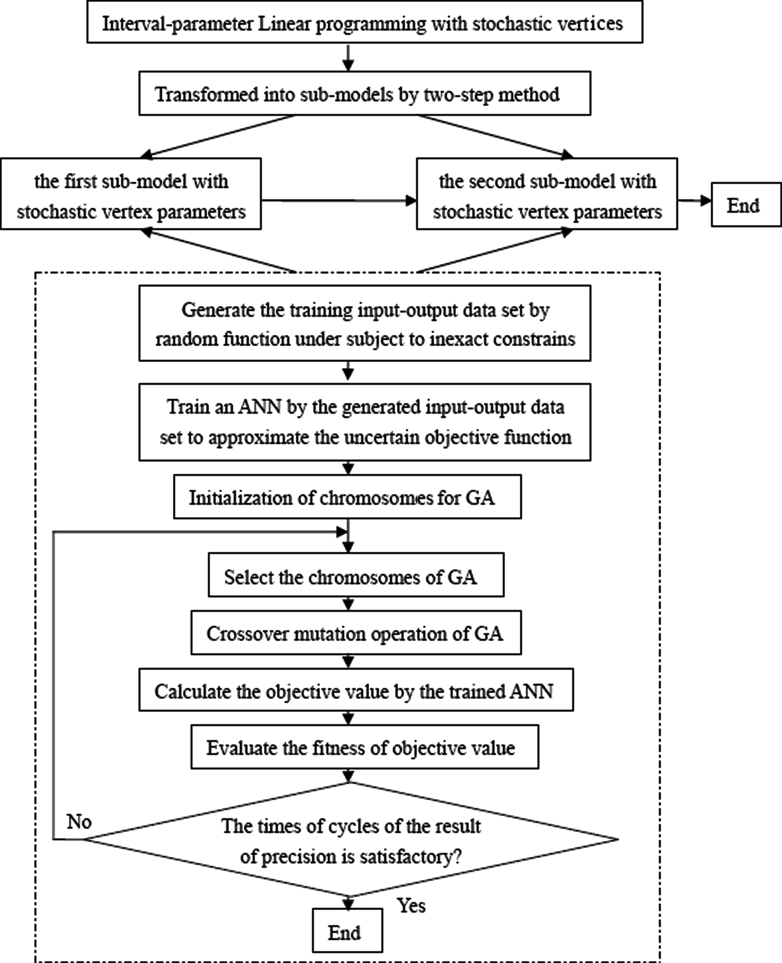
The formulas (3) and (4) are linear programming with stochastic parameters. Because of stochastic parameters in the submodels, it cannot be directly solved by the simplex method. A hybrid intelligent algorithm based on artificial neural network (ANN) and genetic algorithm (GA) was proposed to solve the problem with stochastic parameters. The hybrid intelligent algorithm is based on ANN and GA. First, the training input–output dataset is generated by random function. The dataset consists of decision variable values that satisfy all constraints and corresponding objective values. Then the training dataset is used to develop an ANN model for approximating the uncertain objective function. Finally, the trained network model is used to replace the objective function and the optimal model can then be solved by the GA method. The procedure of hybrid intelligent algorithm for solving the interval-parameter linear programming with stochastic vertices is shown in Fig. 1. The detailed process of solving the submodel with the hybrid intelligent algorithm is as follows:

Step 1: Randomly generate values of decision variables satisfying all constraints, which will be used as input data for training ANN. The objective values corresponding to those decision variables will be used as output data through randomly selecting coefficient values in objective function according to their distribution functions.

Step 2: Train an ANN to approximate the uncertain objective function with the generated input–output training dataset.

Step 3: Initialize population of chromosomes whose feasibility is checked by the constraints.

Step 4: Update the chromosomes by crossover and mutation operations in which the feasibility of offspring may be checked by the constraints.

Step 5: Calculate the objective values for all chromosomes with the trained neural network.

Step 6: Compute the fitness of each chromosome according to the objective values.

Step 7: Select the chromosomes by spinning the roulette wheel.

Step 8: Repeat the fourth to seventh steps for a given iteration time.

Step 9: Report the best chromosomes as the optimal solution.

FIG. 1.

Flow chart hybrid intelligent algorithm for solving the ILPSV model.

There are many ANN models that have been used in a large number of practical fields. In this study, we chose the back propagation ANN models with three layers. The ANN-developing process is coded and integrated within the framework of the hybrid intelligent algorithm. As shown in Fig. 1, inexact constraints of the optimal model will be used to generate the training input–output dataset by random function. Once one group of data of decision variable values is generated, it will be used to check whether all constraints are satisfied or not. If yes, it will be saved as an effective data group for training the ANN model. Otherwise, a new data group will be generated. This process will be repeated till the expected number of effective data groups is obtained.

Illustrative Example

An illustrative example in the work by Li et al. (2010) is quoted to demonstrate the applicability of the proposed method as follows: \documentclass{aastex} \usepackage{amsbsy} \usepackage{amsfonts} \usepackage{amssymb} \usepackage{bm} \usepackage{mathrsfs} \usepackage{pifont} \usepackage{stmaryrd} \usepackage{textcomp} \usepackage{portland, xspace} \usepackage{amsmath, amsxtra} \pagestyle{empty} \DeclareMathSizes {10} {9} {7} {6} \begin{document} \begin{align*} \max \bar{f} = [\xi_1, \xi_2] \overline{x}_1 - [5.5, 6.0] \overline{x}_2 \tag {5a} \end{align*} \end{document} Subject to \documentclass{aastex} \usepackage{amsbsy} \usepackage{amsfonts} \usepackage{amssymb} \usepackage{bm} \usepackage{mathrsfs} \usepackage{pifont} \usepackage{stmaryrd} \usepackage{textcomp} \usepackage{portland, xspace} \usepackage{amsmath, amsxtra} \pagestyle{empty} \DeclareMathSizes {10} {9} {7} {6} \begin{document} \begin{align*} [8, 10] \overline{x}_1 - [12, 14] \overline{x}_2 \leq [3.8, 4.2] \tag {5b} \end{align*} \end{document} \documentclass{aastex} \usepackage{amsbsy} \usepackage{amsfonts} \usepackage{amssymb} \usepackage{bm} \usepackage{mathrsfs} \usepackage{pifont} \usepackage{stmaryrd} \usepackage{textcomp} \usepackage{portland, xspace} \usepackage{amsmath, amsxtra} \pagestyle{empty} \DeclareMathSizes {10} {9} {7} {6} \begin{document} \begin{align*} [\gamma_1, \gamma_2] \overline{x}_1 + [3, 4] \overline{x}_2 \leq [\eta_1, \eta_2] \tag {5c} \end{align*} \end{document} \documentclass{aastex} \usepackage{amsbsy} \usepackage{amsfonts} \usepackage{amssymb} \usepackage{bm} \usepackage{mathrsfs} \usepackage{pifont} \usepackage{stmaryrd} \usepackage{textcomp} \usepackage{portland, xspace} \usepackage{amsmath, amsxtra} \pagestyle{empty} \DeclareMathSizes {10} {9} {7} {6} \begin{document} \begin{align*} \overline{x}_1, \overline{x}_2 \geq 0 \tag {5d} \end{align*} \end{document} Where ξ₁, ξ₂, γ₁, γ₂, η₁, and η₂ are the random variables with uniform distributions of U(26,27), U(29,30), U(2.4,2.5), U(2.7,2.8), U(6.0,6.2), and, U(6.3,6.5), respectively. These vertices were only interval values in the work by Li et al. (2010). The above model can then be converted into the following two submodels: \documentclass{aastex} \usepackage{amsbsy} \usepackage{amsfonts} \usepackage{amssymb} \usepackage{bm} \usepackage{mathrsfs} \usepackage{pifont} \usepackage{stmaryrd} \usepackage{textcomp} \usepackage{portland, xspace} \usepackage{amsmath, amsxtra} \pagestyle{empty} \DeclareMathSizes {10} {9} {7} {6} \begin{document} \begin{align*} \rm max f^U = \xi_2 x_1^U - 5.5x_2^L \tag {6a} \end{align*} \end{document} Subject to \documentclass{aastex} \usepackage{amsbsy} \usepackage{amsfonts} \usepackage{amssymb} \usepackage{bm} \usepackage{mathrsfs} \usepackage{pifont} \usepackage{stmaryrd} \usepackage{textcomp} \usepackage{portland, xspace} \usepackage{amsmath, amsxtra} \pagestyle{empty} \DeclareMathSizes {10} {9} {7} {6} \begin{document} \begin{align*} 8x_1^U - 14x_2^L \leq 4.2 \tag {6b} \end{align*} \end{document} \documentclass{aastex} \usepackage{amsbsy} \usepackage{amsfonts} \usepackage{amssymb} \usepackage{bm} \usepackage{mathrsfs} \usepackage{pifont} \usepackage{stmaryrd} \usepackage{textcomp} \usepackage{portland, xspace} \usepackage{amsmath, amsxtra} \pagestyle{empty} \DeclareMathSizes {10} {9} {7} {6} \begin{document} \begin{align*} \gamma_1 x_1^U + 4x_2^L \leq \eta_2 \tag {6c} \end{align*} \end{document} \documentclass{aastex} \usepackage{amsbsy} \usepackage{amsfonts} \usepackage{amssymb} \usepackage{bm} \usepackage{mathrsfs} \usepackage{pifont} \usepackage{stmaryrd} \usepackage{textcomp} \usepackage{portland, xspace} \usepackage{amsmath, amsxtra} \pagestyle{empty} \DeclareMathSizes {10} {9} {7} {6} \begin{document} \begin{align*} x_1^U, x_2^L \geq 0 \tag {6d} \end{align*} \end{document} and \documentclass{aastex} \usepackage{amsbsy} \usepackage{amsfonts} \usepackage{amssymb} \usepackage{bm} \usepackage{mathrsfs} \usepackage{pifont} \usepackage{stmaryrd} \usepackage{textcomp} \usepackage{portland, xspace} \usepackage{amsmath, amsxtra} \pagestyle{empty} \DeclareMathSizes {10} {9} {7} {6} \begin{document} \begin{align*} \rm max f^L = \xi_1 x_1^L - 6.0x_2^U \tag {7a} \end{align*} \end{document} Subject to \documentclass{aastex} \usepackage{amsbsy} \usepackage{amsfonts} \usepackage{amssymb} \usepackage{bm} \usepackage{mathrsfs} \usepackage{pifont} \usepackage{stmaryrd} \usepackage{textcomp} \usepackage{portland, xspace} \usepackage{amsmath, amsxtra} \pagestyle{empty} \DeclareMathSizes {10} {9} {7} {6} \begin{document} \begin{align*} 10x_1^L - 12x_2^U \leq 3.8 \tag {7b} \end{align*} \end{document} \documentclass{aastex} \usepackage{amsbsy} \usepackage{amsfonts} \usepackage{amssymb} \usepackage{bm} \usepackage{mathrsfs} \usepackage{pifont} \usepackage{stmaryrd} \usepackage{textcomp} \usepackage{portland, xspace} \usepackage{amsmath, amsxtra} \pagestyle{empty} \DeclareMathSizes {10} {9} {7} {6} \begin{document} \begin{align*} \gamma_2 x_1^L + 3x_2^U \leq \eta_1 \tag {7c} \end{align*} \end{document} \documentclass{aastex} \usepackage{amsbsy} \usepackage{amsfonts} \usepackage{amssymb} \usepackage{bm} \usepackage{mathrsfs} \usepackage{pifont} \usepackage{stmaryrd} \usepackage{textcomp} \usepackage{portland, xspace} \usepackage{amsmath, amsxtra} \pagestyle{empty} \DeclareMathSizes {10} {9} {7} {6} \begin{document} \begin{align*} x_1^L \leq x_{\rm 1opt}^U \tag {7d} \end{align*} \end{document} \documentclass{aastex} \usepackage{amsbsy} \usepackage{amsfonts} \usepackage{amssymb} \usepackage{bm} \usepackage{mathrsfs} \usepackage{pifont} \usepackage{stmaryrd} \usepackage{textcomp} \usepackage{portland, xspace} \usepackage{amsmath, amsxtra} \pagestyle{empty} \DeclareMathSizes {10} {9} {7} {6} \begin{document} \begin{align*} x_2^U \geq x_{ \rm 2opt}^L \tag {7e} \end{align*} \end{document} where \documentclass{aastex} \usepackage{amsbsy} \usepackage{amsfonts} \usepackage{amssymb} \usepackage{bm} \usepackage{mathrsfs} \usepackage{pifont} \usepackage{stmaryrd} \usepackage{textcomp} \usepackage{portland, xspace} \usepackage{amsmath, amsxtra} \pagestyle{empty} \DeclareMathSizes {10} {9} {7} {6} \begin{document} $$x_{\rm 1opt}^U$$ \end{document} and \documentclass{aastex} \usepackage{amsbsy} \usepackage{amsfonts} \usepackage{amssymb} \usepackage{bm} \usepackage{mathrsfs} \usepackage{pifont} \usepackage{stmaryrd} \usepackage{textcomp} \usepackage{portland, xspace} \usepackage{amsmath, amsxtra} \pagestyle{empty} \DeclareMathSizes {10} {9} {7} {6} \begin{document} $$x_{\rm 2opt}^L$$ \end{document} are solutions from submodel (6). For models (6) and (7), the ANN and GA were employed to produce a hybrid intelligent algorithm for solving SP models. A running of the hybrid intelligent algorithm (200 iteration simulations, 500 data in ANN, and 50 generations in GA) was undertaken to solve the two submodels.

With the hybrid intelligent algorithm, the solutions of model (6) are \documentclass{aastex} \usepackage{amsbsy} \usepackage{amsfonts} \usepackage{amssymb} \usepackage{bm} \usepackage{mathrsfs} \usepackage{pifont} \usepackage{stmaryrd} \usepackage{textcomp} \usepackage{portland, xspace} \usepackage{amsmath, amsxtra} \pagestyle{empty} \DeclareMathSizes {10} {9} {7} {6} \begin{document} $$x_1^U = 1.6084$$ \end{document} and \documentclass{aastex} \usepackage{amsbsy} \usepackage{amsfonts} \usepackage{amssymb} \usepackage{bm} \usepackage{mathrsfs} \usepackage{pifont} \usepackage{stmaryrd} \usepackage{textcomp} \usepackage{portland, xspace} \usepackage{amsmath, amsxtra} \pagestyle{empty} \DeclareMathSizes {10} {9} {7} {6} \begin{document} $$x_2^L = 0.6195$$ \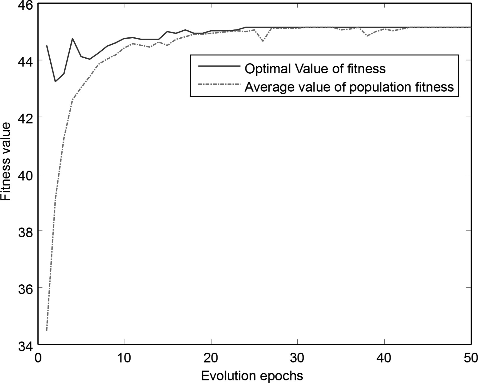end{document} , and the corresponding objective value is f^U = 45.1408 (Fig. 2).

FIG. 2.

Evolution process of upper bound of objective function by genetic algorithm (GA).

Then the solutions of model (7) are obtained: \documentclass{aastex} \usepackage{amsbsy} \usepackage{amsfonts} \usepackage{amssymb} \usepackage{bm} \usepackage{mathrsfs} \usepackage{pifont} \usepackage{stmaryrd} \usepackage{textcomp} \usepackage{portland, xspace} \usepackage{amsmath, amsxtra} \pagestyle{empty} \DeclareMathSizes {10} {9} {7} {6} \begin{document} $$x_1^L = 1.3153, x_2^U = 0.7797$$ \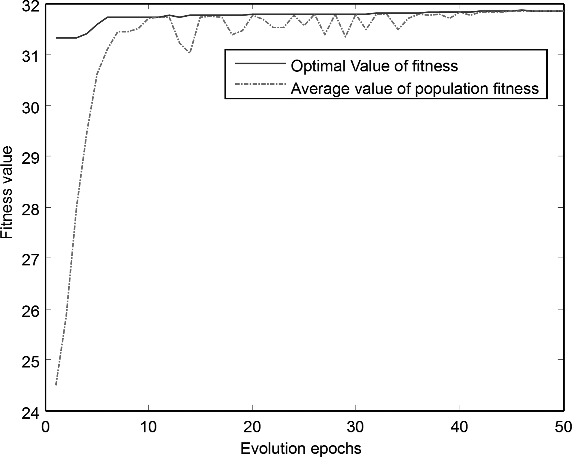end{document} , and the corresponding objective value is f^L = 31.8582 (Fig. 3).

FIG. 3.

Evolution process of lower bound of objective function by GA.

Therefore, the solutions of problem (5) are \documentclass{aastex} \usepackage{amsbsy} \usepackage{amsfonts} \usepackage{amssymb} \usepackage{bm} \usepackage{mathrsfs} \usepackage{pifont} \usepackage{stmaryrd} \usepackage{textcomp} \usepackage{portland, xspace} \usepackage{amsmath, amsxtra} \pagestyle{empty} \DeclareMathSizes {10} {9} {7} {6} \begin{document} $$\overline{x}_{\rm 1opt} = [1.3153, 1.6084], \overline{x}_{\rm 2opt} = [0.6195, 0.7797]$$ \end{document} , and the corresponding objective value is \documentclass{aastex} \usepackage{amsbsy} \usepackage{amsfonts} \usepackage{amssymb} \usepackage{bm} \usepackage{mathrsfs} \usepackage{pifont} \usepackage{stmaryrd} \usepackage{textcomp} \usepackage{portland, xspace} \usepackage{amsmath, amsxtra} \pagestyle{empty} \DeclareMathSizes {10} {9} {7} {6} \begin{document} $$\overline{f}_{\rm opt} = [31.8582, 45.1408].$$ \end{document} In the work by Li et al. (2010), ξ₁, ξ₂, γ₁, γ₂, η₁, and η₂ were interval values, and the DIV method was employed. The solution from their work and that from the ILPSV method in this study are listed in Table 1.

Table 1.

Results of Using ILP, Dual-Interval Vertex, and ILPSV Methods

Methods	ILP	DIV	ILPSV
Objective value	[[29.438, 32.150], [42.172, 45.784]]	[[30.099, 31.455], [43.053, 44.895]]	[31.858, 45.141]

ILP, interval-parameter linear programming; DIV, dual-interval vertex; ILPSV, interval-parameter linear programming with stochastic vertices.

Table 1 also lists the solution of objective value of the model (5) with ILP method through considering the coefficients as dual interval parameters. It presents that the lower and upper bounds of the objective value from the ILPSV lie in the interval of the lower and upper bounds from the ILP. The reason is that interval parameters with stochastic vertices of coefficient have less uncertainty degree than those of dual interval parameters, so that the uncertainty degree of the solution from the ILPSV is also less. Comparing solutions from DIV and ILPSV, it shows that some objective values from ILPSV are not included in the results from DIV. It might result from solving the algorithm by a discrete way so that some feasible solutions are missed. Moreover, the lower bound (31.858) of objective values of ILPSV in Table 1 is greater than the interval ([30.099, 31.455]) of lower bound of DIV in Table 1, because uniform distribution of lower and upper bounds of the interval parameter has more information than that of DIV. Therefore, the developed ILPSV with the hybrid intelligent algorithm can be effectively used for solving dual uncertainty problems with interval parameters with fuzzy or stochastic vertices.

Application

Overview of the study area

The Hetao irrigation region, which is located in the south of the BaYanNaoer city in Inner Mongolia Municipality, is the third largest irrigation region in China. The Hetao irrigation region lies in an extreme arid area, with average annual rainfall being only 150 mm, and the average yearly evaporation is from 2157 to 3178 mm. The area of the Hetao irrigation region is 57.44 × 10⁴ hm², in which 52.47 × 10⁴ hm² is for farm land and 4.97 × 10⁴ hm² is for forest and grassland. The primary crops include wheat, corn, beet, oil crop, oil sunflower, melon, and fruit. Grain, oil crop, and sugar are the traditional preponderant crops. At present, the Hetao irrigation region has become the major product region of grain, oil crop, and sugar in Inner Mongolia Municipality.

Irrigation water for the Hetao region is mainly transferred from the Yellow River. Because of the historical and practical reasons, agriculture irrigation is always the largest user of water resources in the Hetao irrigation region. The average water consumption is 5 billion cubic meters, which is one-sixth of the Yellow River runoff. Currently, the total water consumption has exceeded the water supply capacity by 1 billion cubic meters. With further socioeconomic development in the Hetao region, water deficiency issue will become more serious. Therefore, efficient land-use and water resources management for agriculture is needed.

Development of ILPSV optimization model for crops land and water resources management

In the Hetao irrigation region, dominant crops include wheat, corn, cereal crops, and so on. There are different benefits on planting different crops with different allocated water. The maximum net benefit of agriculture production is taken as the objective of water resources allocation and land-use management. The objective function is subject to 13 constraints, including total water supply capacity constraint, as formula (8b); total farm land area constraint, as formula (8c); minimal crop production requirement, as formula (8d); and each crop planting area constraint, as formula (8e). The developed ILPSV optimization model for land uses of crops planting and water resources allocation is given as follows: \documentclass{aastex} \usepackage{amsbsy} \usepackage{amsfonts} \usepackage{amssymb} \usepackage{bm} \usepackage{mathrsfs} \usepackage{pifont} \usepackage{stmaryrd} \usepackage{textcomp} \usepackage{portland, xspace} \usepackage{amsmath, amsxtra} \pagestyle{empty} \DeclareMathSizes {10} {9} {7} {6} \begin{document} \begin{align*} \max \bar{f} = \sum_{i = 1}^n \overline{C}_i \overline{X}_i \tag {8a} \end{align*} \end{document} Subject to \documentclass{aastex} \usepackage{amsbsy} \usepackage{amsfonts} \usepackage{amssymb} \usepackage{bm} \usepackage{mathrsfs} \usepackage{pifont} \usepackage{stmaryrd} \usepackage{textcomp} \usepackage{portland, xspace} \usepackage{amsmath, amsxtra} \pagestyle{empty} \DeclareMathSizes {10} {9} {7} {6} \begin{document} \begin{align*} \sum_{i = 1}^n \overline{A}_i \overline{X}_i \leq \overline{\eta} \quad \hbox{(total water supply capacity constraint )} \tag {8b} \end{align*} \end{document} \documentclass{aastex} \usepackage{amsbsy} \usepackage{amsfonts} \usepackage{amssymb} \usepackage{bm} \usepackage{mathrsfs} \usepackage{pifont} \usepackage{stmaryrd} \usepackage{textcomp} \usepackage{portland, xspace} \usepackage{amsmath, amsxtra} \pagestyle{empty} \DeclareMathSizes {10} {9} {7} {6} \begin{document} \begin{align*} \sum_{i = 1}^n \overline{X}_i \leq \overline{L} \quad \hbox{(total farm land area constraint)} \tag {8c} \end{align*} \end{document} \documentclass{aastex} \usepackage{amsbsy} \usepackage{amsfonts} \usepackage{amssymb} \usepackage{bm} \usepackage{mathrsfs} \usepackage{pifont} \usepackage{stmaryrd} \usepackage{textcomp} \usepackage{portland, xspace} \usepackage{amsmath, amsxtra} \pagestyle{empty} \DeclareMathSizes {10} {9} {7} {6} \begin{document} \begin{align*} \sum_{i = 1}^k \overline{P}_i \overline{X}_i [ \tau^L, \tau^U] \geq \overline{R} \enspace \hbox{(minimal crop production requirement)}\tag {8d} \end{align*} \end{document} \documentclass{aastex} \usepackage{amsbsy} \usepackage{amsfonts} \usepackage{amssymb} \usepackage{bm} \usepackage{mathrsfs} \usepackage{pifont} \usepackage{stmaryrd} \usepackage{textcomp} \usepackage{portland, xspace} \usepackage{amsmath, amsxtra} \pagestyle{empty} \DeclareMathSizes {10} {9} {7} {6} \begin{document} \begin{align*} B_i^L \leq \overline{X}_i \leq B_i^U \quad \hbox{(planting area limit for each crop)} \tag{8e} \end{align*} \end{document} where \documentclass{aastex} \usepackage{amsbsy} \usepackage{amsfonts} \usepackage{amssymb} \usepackage{bm} \usepackage{mathrsfs} \usepackage{pifont} \usepackage{stmaryrd} \usepackage{textcomp} \usepackage{portland, xspace} \usepackage{amsmath, amsxtra} \pagestyle{empty} \DeclareMathSizes {10} {9} {7} {6} \begin{document} $$\overline{X}_i (i = 1, 2, 3, \ldots, n)$$ \end{document} denotes land area for each crop planting; n = 10 is the total number of crop types, including grain crops (wheat, corn, Summer cereal crops, Fall cereal crops, and interplanting) and cash crops (sunflower, oil crop, beet, fruit tree, and grassland). \documentclass{aastex} \usepackage{amsbsy} \usepackage{amsfonts} \usepackage{amssymb} \usepackage{bm} \usepackage{mathrsfs} \usepackage{pifont} \usepackage{stmaryrd} \usepackage{textcomp} \usepackage{portland, xspace} \usepackage{amsmath, amsxtra} \pagestyle{empty} \DeclareMathSizes {10} {9} {7} {6} \begin{document} $$\overline{C}_i$$ \end{document} is the net benefit coefficient of i crop. \documentclass{aastex} \usepackage{amsbsy} \usepackage{amsfonts} \usepackage{amssymb} \usepackage{bm} \usepackage{mathrsfs} \usepackage{pifont} \usepackage{stmaryrd} \usepackage{textcomp} \usepackage{portland, xspace} \usepackage{amsmath, amsxtra} \pagestyle{empty} \DeclareMathSizes {10} {9} {7} {6} \begin{document} $$\overline{A}_i$$ \end{document} is the water demand coefficient of i crop. \documentclass{aastex} \usepackage{amsbsy} \usepackage{amsfonts} \usepackage{amssymb} \usepackage{bm} \usepackage{mathrsfs} \usepackage{pifont} \usepackage{stmaryrd} \usepackage{textcomp} \usepackage{portland, xspace} \usepackage{amsmath, amsxtra} \pagestyle{empty} \DeclareMathSizes {10} {9} {7} {6} \begin{document} $$\overline{\eta} = [\eta^L, \eta^U]$$ \end{document} , where η^L and η^U are the lower and upper bounds of total available water resources amount for irrigation transferred from the Yellow River, which are normal distribution random variables N(4.700 × 10⁹,0.001) and N(5.000 × 10⁹,0.001), respectively. \documentclass{aastex} \usepackage{amsbsy} \usepackage{amsfonts} \usepackage{amssymb} \usepackage{bm} \usepackage{mathrsfs} \usepackage{pifont} \usepackage{stmaryrd} \usepackage{textcomp} \usepackage{portland, xspace} \usepackage{amsmath, amsxtra} \pagestyle{empty} \DeclareMathSizes {10} {9} {7} {6} \begin{document} $$\overline{L}$$ \end{document} is the area of total farm land, [1,125.40, 1,125.42] × 10⁴ acres. \documentclass{aastex} \usepackage{amsbsy} \usepackage{amsfonts} \usepackage{amssymb} \usepackage{bm} \usepackage{mathrsfs} \usepackage{pifont} \usepackage{stmaryrd} \usepackage{textcomp} \usepackage{portland, xspace} \usepackage{amsmath, amsxtra} \pagestyle{empty} \DeclareMathSizes {10} {9} {7} {6} \begin{document} $$\overline{P}_i$$ \end{document} is the production coefficient of i grain crop. k = 5 is the total number of grain crops. \documentclass{aastex} \usepackage{amsbsy} \usepackage{amsfonts} \usepackage{amssymb} \usepackage{bm} \usepackage{mathrsfs} \usepackage{pifont} \usepackage{stmaryrd} \usepackage{textcomp} \usepackage{portland, xspace} \usepackage{amsmath, amsxtra} \pagestyle{empty} \DeclareMathSizes {10} {9} {7} {6} \begin{document} $$\overline{R}$$ \end{document} is the total yield requirement of grain crop, [280, 320] × 10⁴ kg. \documentclass{aastex} \usepackage{amsbsy} \usepackage{amsfonts} \usepackage{amssymb} \usepackage{bm} \usepackage{mathrsfs} \usepackage{pifont} \usepackage{stmaryrd} \usepackage{textcomp} \usepackage{portland, xspace} \usepackage{amsmath, amsxtra} \pagestyle{empty} \DeclareMathSizes {10} {9} {7} {6} \begin{document} $$\overline{\tau} = [\tau^L, \tau^U]$$ \end{document} , where τ^L and τ^U are the lower and upper bounds of impact coefficient from climate changing on crop production, which are uniform distribution random variables U(0.97,0.99) and U(0.98,1.00), respectively. \documentclass{aastex} \usepackage{amsbsy} \usepackage{amsfonts} \usepackage{amssymb} \usepackage{bm} \usepackage{mathrsfs} \usepackage{pifont} \usepackage{stmaryrd} \usepackage{textcomp} \usepackage{portland, xspace} \usepackage{amsmath, amsxtra} \pagestyle{empty} \DeclareMathSizes {10} {9} {7} {6} \begin{document} $$\overline{B} = [B^L, B^U]$$ \end{document} where \documentclass{aastex} \usepackage{amsbsy} \usepackage{amsfonts} \usepackage{amssymb} \usepackage{bm} \usepackage{mathrsfs} \usepackage{pifont} \usepackage{stmaryrd} \usepackage{textcomp} \usepackage{portland, xspace} \usepackage{amsmath, amsxtra} \pagestyle{empty} \DeclareMathSizes {10} {9} {7} {6} \begin{document} $$B_i^L$$ \end{document} and \documentclass{aastex} \usepackage{amsbsy} \usepackage{amsfonts} \usepackage{amssymb} \usepackage{bm} \usepackage{mathrsfs} \usepackage{pifont} \usepackage{stmaryrd} \usepackage{textcomp} \usepackage{portland, xspace} \usepackage{amsmath, amsxtra} \pagestyle{empty} \DeclareMathSizes {10} {9} {7} {6} \begin{document} $$B_i^U$$ \end{document} are the lower and upper bounds of i crop planting area limit. Table 2 shows the coefficients and parameters in model (8).

Table 2.

Coefficients of Model and Planting Area Limit for Each Crop

Crop type		\documentclass{aastex} \usepackage{amsbsy} \usepackage{amsfonts} \usepackage{amssymb} \usepackage{bm} \usepackage{mathrsfs} \usepackage{pifont} \usepackage{stmaryrd} \usepackage{textcomp} \usepackage{portland, xspace} \usepackage{amsmath, amsxtra} \pagestyle{empty} \DeclareMathSizes {10} {9} {7} {6} \begin{document} $$\overline{C}_i$$ \end{document} (RMB/acre)	\documentclass{aastex} \usepackage{amsbsy} \usepackage{amsfonts} \usepackage{amssymb} \usepackage{bm} \usepackage{mathrsfs} \usepackage{pifont} \usepackage{stmaryrd} \usepackage{textcomp} \usepackage{portland, xspace} \usepackage{amsmath, amsxtra} \pagestyle{empty} \DeclareMathSizes {10} {9} {7} {6} \begin{document} $$\overline{A}_i$$ \end{document} (m³/acre)	\documentclass{aastex} \usepackage{amsbsy} \usepackage{amsfonts} \usepackage{amssymb} \usepackage{bm} \usepackage{mathrsfs} \usepackage{pifont} \usepackage{stmaryrd} \usepackage{textcomp} \usepackage{portland, xspace} \usepackage{amsmath, amsxtra} \pagestyle{empty} \DeclareMathSizes {10} {9} {7} {6} \begin{document} $$\overline{P}_i$$ \end{document} (10³ kg/acre)	\documentclass{aastex} \usepackage{amsbsy} \usepackage{amsfonts} \usepackage{amssymb} \usepackage{bm} \usepackage{mathrsfs} \usepackage{pifont} \usepackage{stmaryrd} \usepackage{textcomp} \usepackage{portland, xspace} \usepackage{amsmath, amsxtra} \pagestyle{empty} \DeclareMathSizes {10} {9} {7} {6} \begin{document} $$\overline{B}_i$$ \end{document} (10⁴ acres)
Grain crops	Wheat	[652, 660]	[330, 340]	[0.33, 0.39]	[250, 500]
	Corn	[745, 758]	[356, 366]	[0.52, 0.56]	[10, 200]
	Summer cereal Crops	[596, 605]	[250, 260]	[0.31, 0.37]	[15, 150]
	Fall cereal crops	[645, 655]	[320, 326]	[0.38, 0.42]	[10, 150]
	Interplanting	[1,138, 1,145]	[460, 469]	[0.54, 0.58]	[100, 350]
Cash crops	Sunflower	[870, 878]	[342, 347]		[50, 200]
	Oil crop	[978, 988]	[360, 370]		[10, 150]
	Beet	[1,028, 1,037]	[392, 403]		[0, 150]
	Fruit tree	[998, 1,005]	[270, 276]		[0, 250]
	Grassland	[145, 155]	[370, 373]		[10, 100]

RMB, monetary symbol in China.

The developed ILPSV is an interval-parameter linear programming model with dual uncertainty of stochastic vertices. To solve the model, first, formula (8) was transferred into two submodels with stochastic parameters. Then, the hybrid intelligent algorithm was employed to solve the submodels. An ANN was established after 500 times of iteration simulation with generated 100 datasets. In the process of GA evolution, the initial population size was 60, the decimal coding was adopted, the probability of selection was set as 0.95, the probability of crossover was 0.85, and the probability of mutation was 0.30. After 50 generations iteration, the solution of the developed model was obtained.

Results and Discussion

Currently, the total water amount transferred from the Yellow River is nearly 5 billion cubic meters, which exceeds the allowable water amount by 1 billion cubic meters. Moreover, the available water from the Yellow River might be reduced with water resources decreasing from the upper Yellow River basin. Therefore, it is necessary to undertake crop planting area optimization under different available water amounts from the Yellow River. The crops planting areas by the developed ILPSV model under different scenarios of water amount transferred from the Yellow River are shown in Table 3.

Table 3.

Crop Planting Areas Under the Three Scenarios of Available Water Amount

	Crops planting areas (acres)
	Scenario 1	Scenario 2	Scenario 3
	[4.700, 5.000] ^a	[4.100, 4.409] ^a	[3.400, 3.606] ^a
Wheat	[3,210,747.04, 3,211,755.52]	[3,085,071.15, 3,131,981.00]	[3,335,907.61, 3,509,253.73]
Corn	[345,977.35, 346,689.99]	[193,976.22, 260,235.03]	[107,419.48, 112,676.56]
Summer cereal crops	[303,262.55, 310,730.36]	[676,017.27, 715,544.21]	[1,170,899.39, 1,436,658.82]
Fall cereal crops	[339,813.04, 342,468.11]	[208,085.03, 246,404.30]	[309,159.05, 381,445.17]
Interplanting	[3,460,152.56, 3,460,692.34]	[3,317,454.88, 3,352,080.31]	[2,604,160.37, 2,753,992.67]
Sunflower	[576,150.66, 579,309.60]	[983,588.88, 1,057,767.80]	[665,173.96, 763,773.04]
Oil crop	[476,960.86, 479,458.44]	[881,855.13, 928,530.97]	[104,682.20, 106,486.96]
Beet	[1,321,681.21, 1,323,385.67]	[788,398.07, 827,835.95]	[13,402.74, 41,456.55]
Fruit tree	[1,028,778.04, 1,030,778.03]	[545,332.93, 586,197.70]	[1,031,268.75, 1,093,396.28]
Grassland	[150,719.35, 168,839.21]	[123,920.86, 147,590.32]	[115,548.02, 134,964.22]

Available water amount (billion cubic meters).

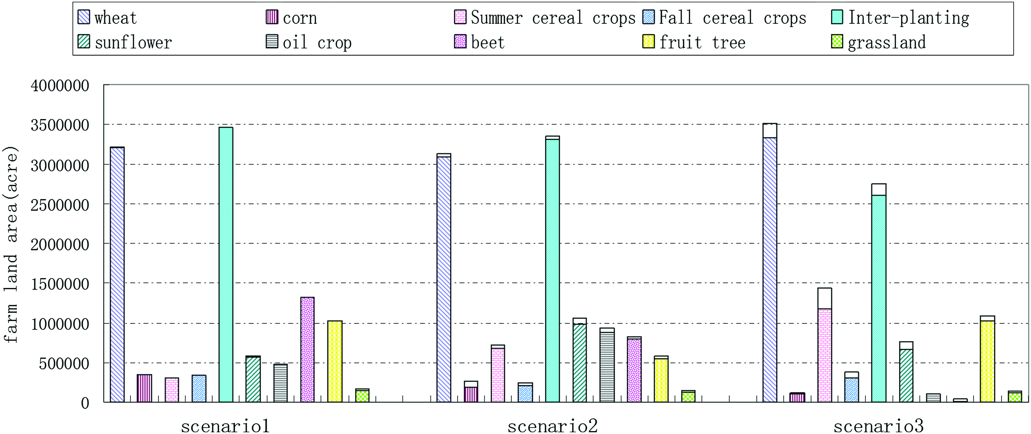
Table 3 presents that interplanting and wheat are main cultivation crops in the study area. In scenario 1, the planting areas of interplanting and wheat are [3,460,152.56, 3,460,692.34] and [3,210,747.04, 3,211,755.52] acres, respectively. Because of high water demand, the interplanting area is gradually declining with decreasing of water transferred from the Yellow River so that its area is [2,604,160.37, 2,753,992.67] acres in scenario 3. As the main wheat-producing region in China, wheat production is paid more attention in the Hetao irrigation region. Therefore, the planting area of wheat keeps a steady extent. Because of relatively high benefit, the beet planting area is also high in the Hetao irrigation region in scenario 1, which is [1,321,681.21, 1,323,385.67] acres. However, the water demand of unit beet planting area is also relatively high so that its planting area is decreased to [13,402.74, 41,456.55] acres in scenario 3. The summer cereal crops area is significantly increased from [303,262.55, 310,730.36] acres in scenario 1 to [1,170,899.39, 1,436,658.82] acres in scenario 3 because of its low water demand. It indicates that water demand of unit planting area has great impact on planting area of each crop. Because of shortage of water resources, the higher the water demand of crop, the lower will be the planting area. The amount of transferred water from the Yellow River affects not only the planting structure of crop but also economy development in the Hetao irrigation region. The net benefit of agriculture is [9,498,183,972, 10,047,337,652] RMB under scenario 1, whereas it is only [7,787,967,089, 8,484,605,881] RMB under scenario 3. The planting areas of crops under different scenarios are shown in Fig. 4.

FIG. 4.

Crop planting area under different water transfer scenario. Color images available online at www.liebertonline.com/ees

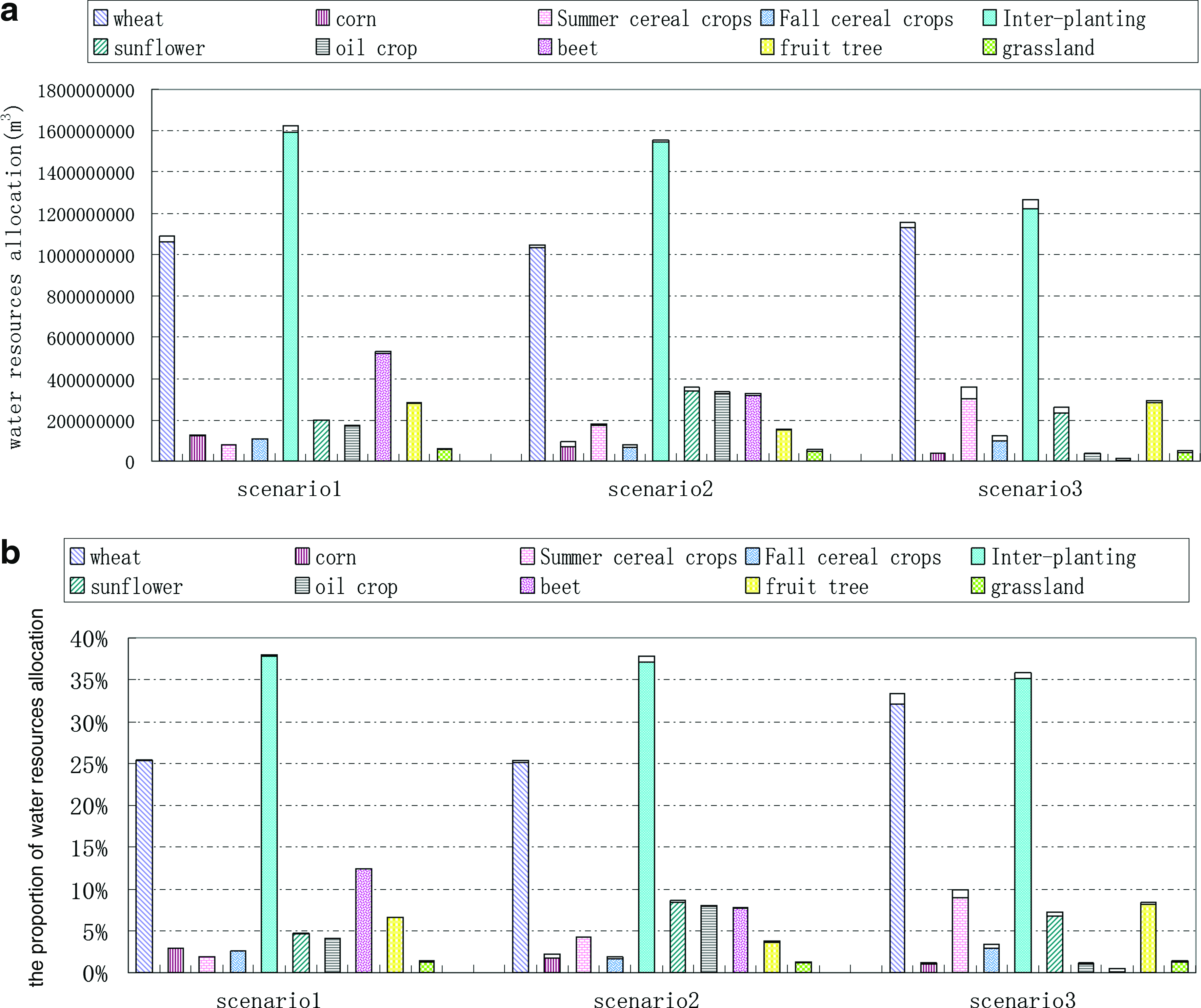
Table 4 presents the allocated water amount to each crop under different scenarios of available water resources from the Yellow River. The allocated water for interplanting is always the highest in the three scenarios. For example, it is [1,591,918,476, 1,622,811,551] cubic meters in scenario 1, which accounts for [37.8, 38.0]% of total allocated water amount; it is [1,541,956,943, 1,555,886,339] cubic meters in scenario 2, which accounts for [37.1, 37.8]%; it is [1,221,351,214, 1,266,836,628] cubic meters in scenario 3, which accounts for [35.1, 35.9]%. Figure 5a and 5b present water resources allocation amount and its' proportion among crops under different scenarios of water amount transferred from the Yellow River, respectively.

FIG. 5.

Results of water allocation to crops under different scenarios of water transfer. Color images available online at www.liebertonline.com/ees

Table 4.

Water Resources Allocation to Each Crop Under the Three Scenarios

	Water resources allocation (cubic meters)
	Scenario 1	Scenario 2	Scenario 3
	[4.700, 5.000] ^a	[4.100 4.409] ^a	[3.400 3.606] ^a
Wheat	[1,059,879,322, 1,091,653,994]	[1,033,553,730, 1,048,924,191]	[1,134,208,587, 1,158,053,731]
Corn	[123,421,636, 126,627,710]	[70,995,296, 92,643,670]	[39,315,529, 40,112,855]
Summer cereal, crops	[77,682,590, 78,848,263]	[175,764,490, 178,886,052]	[304,433,841, 359,164,705]
Fall cereal crops	[109,589,795, 110,779,051]	[67,835,719, 78,849,376]	[100,785,850, 122,062,454]
Interplanting	[1,591,918,476, 1,622,811,551]	[1,541,956,943, 1,555,886,339]	[1,221,351,214, 1,266,836,628]
Sunflower	[198,123,883, 199,924,279]	[341,305,341, 361,756,587]	[230,815,364, 261,210,380]
Oil crop	[172,605,038, 176,475,518]	[326,286,398, 334,271,149]	[38,335,305, 38,732,414]
Beet	[518,767,183, 532,637,527]	[317,724,422, 324,511,692]	[5,401,304, 16,250,967]
Fruit tree	[278,310,068, 283,942,739]	[150,511,888, 158,273,379]	[284,630,175, 295,216,996]
Grassland	[56,218,317, 62,470,507]	[46,222,480, 54,608,418]	[43,099,411, 49,936,761]

Available water amount (billion cubic meters).

With decreasing of available water transferred from the Yellow River, the allocated water for interplanting is gradually reduced because of its highest water demand. In scenario 1, water resources transferred from the Yellow River is [4.700, 5.000] billion cubic meters, which is abundant, and so water is not a scarce resource for all crops. Water requirements of all corps can be met. The relatively high-water-consumption crop, such as beet, will be fully planted in the Hetao irrigation region. The allocated water to beet is [518,767,183, 532,637,527] cubic meters, which accounts for [12.39, 12.42]% of the total water used. In scenario 2, total amount of water transferred from the Yellow River is [4.100, 4.409] billion cubic meters. Correspondingly, water amount allocated for beet is [317,724,422, 324,511,692] cubic meters, being reduced by [201,042,761, 208,125,835] cubic meters. The water amount transferred from the Yellow River is only [3.400, 3.606] billion cubic meters in scenario 3, which presents water scarcity scheme. The planting areas of high-water-consumption crops will be significantly cut down because of decrease in available water amount. Correspondingly, the allocated water to beet is [5,401,304, 16,250,967] cubic meters, which only accounts for [0.001, 0.004]% of total water used. Similarly, water amounts allocated to oil crop and grassland have same changing trend with water supply decreasing. Contrarily, with water supply decreasing, planting area of summer cereal crops is gradually increased because of its lowest water demand. The allocated water amount for summer cereal crops is [77,682,590, 78,848,263] cubic meters in scenario 1, which accounts for [1.83, 1.85]% of all water used. However, it is [304,433,841, 359,164,705] cubic meters in scenario 3, which accounts for [8.95, 8.96]%. The results indicate that the planting areas of high-water-demand crops will be reduced gradually and those of low-water-demand crops will be increased with available water decreasing.

SP is a mathematical program in which an optimal model has uncertain coefficients and parameters in the objective function and constraints with probability distributions. If probability distribution functions of uncertain coefficients and parameters can be obtained, it will be effective to solve the problems. For many practical problems, information on probability distribution of coefficients and parameters of objective function and constraints is hard to be obtained. Therefore, the interval-parameter linear programming (ILP) has been developed to deal with problems in which uncertain coefficients and parameters can only be presented as interval numbers. Moreover, the lower and upper bounds of interval number can also be uncertain with stochastic or fuzzy distribution. For this kind of problems, both SP and ILP methods might not be effective to obtain idea solutions. Therefore, a new effective way is desired to solve this problem. In this article, the ILPSV method is developed based on the ILP method and a hybrid intelligent algorithm is proposed for solving the ILPSV model. It combines advantages of both SP and ILP methods.

Both the results of the illustrative example and field application indicate that the developed hybrid intelligent algorithm based on ANN and GA for solving optimal models with dual uncertain coefficients and parameters can overcome the disadvantage of the DIV method that some feasible solutions are missed. The whole solving process with the developed algorithm can be completed with a program. Therefore, it can avoid heavy and complex user operation. The disadvantage of the developed method in this article is that the solution accuracy depends on the simulation accuracy of the ANN model. Future research is desired to improve the simulation accuracy of the ANN model so that the accuracy of optimal solutions can be ensured.

Conclusion

In this article, an interval-parameter linear programming with stochastic vertices (ILPSV) model has been developed. A hybrid intelligent algorithm, which is based on ANN and GA, has been proposed for solving the developed model. The developed methodology can deal with dual uncertainties presented as interval-parameter with stochastic vertices that exist in both objective function and left- and right-hand sides of constraints. The results of an illustrative example with the developed method indicated that the proposed ILPSV with hybrid intelligent algorithm can overcome the shortage of previous discrete methods, which might miss some feasible solutions. The developed model was then applied to the allocation of land and water resources among different crops in the Hetao irrigation region in China. The results indicated that water amount transferred from the Yellow River directly affected both planting structure and economy development in the Hetao irrigation region. The planting areas of high-water-demand crops would be gradually transferred into those of low-water-demand crops with decreasing of water amount transferred from the Yellow River. The application of the developed methodology showed that it is an effective method to deal with dual uncertainty problems in a land-use and water resources management system. It might help authorities better understand the system complexity and effectively make the planning of land and water resources management strategies.

Footnotes

Acknowledgments

This research has been supported by the National Basic Research Program of China (973 Program) (No. 2005CB724202), China Postdoctoral Science Foundation-funded project (No. 20090460358), and the R&D Special Fund for Public Welfare Industry of Ministry of Water Resources in China (No. 200701008). The authors are grateful to the editor and the anonymous reviewers for their insightful and helpful comments and suggestions.

Author Disclosure Statement

No competing financial interests exist.

References

Abrishamchi

, Marino

M.A.

, Afshar

1991. Reservoir planning for irrigation district. J. Water Resour. Plann. Manage., 117:74.

Acevedo

, Pistikopoulos

E.N.

1998. Stochastic optimization based algorithms for process synthesis under uncertainty. Comput. Chem. Eng., 22:647.

Andersen

P.P.

1997. The world food situation: recent developments, emerging issues, and long-term prospects. Food Policy Report. Washington, DC: International Food Policy Research Institute, 36.

Beaumont

1998. Solving interval linear systems with linear programming techniques. Linear Algebra Appl., 281:293.

Chang

N.B.

, Wen

C.G.

, Wu

S.L.

1994. Optimal management of environmental and land resources in a reservoir watershed by multi-objective programming. J. Environ. Manage., 44:145.

Huang

G.H.

1996. IPWM: an interval parameter water quality management model. Eng. Optimizat., 26:79.

Huang

G.H.

, Baetz

B.W.

, Patry

G.G.

1992. A grey linear programming approach for municipal solid waste management planning under certainty. Civ. Eng. Syst., 9:319.

Huang

G.H.

, Baetz

B.W.

, Patry

G.G.

1993. A grey fuzzy linear programming approach for municipal solid waste management planning under uncertainty. Civ. Eng. Syst., 10:123.

Huang

G.H.

, Beatz

B.W.

, Patry

G.G.

1995. Grey integer programming: an application to waste management planning under uncertainty. Eur. J. Oper. Res., 83:594.

10.

Huang

G.H.

, Loucks

D.P.

2000. An inexact two-stage stochastic programming model for water resources management under uncertainty. Civ. Eng. Environ. Syst., 17:95.

11.

Kindler

1992. Rationalizing water requirements with aid of fuzzy allocation model. J. Water Resour. Plann. Manage., 118:308.

12.

Y.P.

, Huang

G.H.

, Guo

, Yang

Z.F.

, Nie

S.L.

2010. A dual-interval vertex analysis method and its application to environmental decision making under uncertainty. Eur. J. Oper. Res., 200:536.

13.

Y.P.

, Huang

G.H.

, Nie

S.L.

2006. An interval-parameter multi-stage stochastic programming model for water resources management under uncertainty. Adv. Water Resour., 29:776.

14.

Y.P.

, Huang

G.H.

, Yang

Z.F.

, Nie

S.L.

2008. IFMP: interval-fuzzy multistage programming for water resources management under uncertainty. Resour. Conser. Recycling, 52:800.

15.

Liu

B.D.

2002. Theory and Practice of Uncertain Programming. Heidelberg: Physica-Verlag.

16.

Liu

B.D.

2009. Theory and Practice of Uncertain Programming, 3rd. Berlin: Springer-Verlag.

17.

Liu

, Qin

X.S.

, Guo

H.C.

, Zhou

, Lv

X.J.

2007. ICCLP: an inexact chance-constrained linear programming model for land-use management of lake areas in urban fringes. Environ. Manage., 40:966.

18.

Liu

, Yu

Y.J.

, Guo

H.C.

, Yang

P.J.

2009. Optimal land-use management for surface source water protection under uncertainty: a case study of Songhuaba watershed (Southwestern China) Water Resour. Manage., 23:2069.

19.

J.Q.

, Chen

S.Y.

, Qiu

2004. A multi-objective fuzzy optimization model for cropping structure and water resources and its method. Agric. Sci. Technol., 5:5.

20.

Mainuddin

, Gupta

A.D.

, Onta

P.R.

1996. Optimal crop planning model for an existing groundwater irrigation project in Thailand. Agric. Water Manage., 33:43.

21.

Maqsood

, Huang

G.H.

, Yeomans

J.S.

2005. An interval-parameter fuzzy two-stage stochastic program for water resources management under uncertainty. Eur. J. Oper. Res., 167:208.

22.

Onta

P.R.

, Loof

, Banskota

1995. Performance based irrigation planning under water shortage. Irrig. Drain. Syst., 9:143.

23.

Paul

, Panda

S.N.

, Kumar

D.N.

2000. Optimal irrigation allocation: a multilevel approach. J. Irrig. Drain. Eng., 126:149.

24.

Sadeghi

S.H.R.

, Jalili

, Nikkami

2009. Land use optimization in watershed scale. Land Use Policy, 26:186.

25.

Vedula

, Mujumdar

P.P.

1992. Optimal reservoir operation for irrigation of multiple crops. Water Resour. Res., 28:1.

26.

Yaron

, Dinar

1982. Optimum allocation of farm irrigation water during peak seasons. Am. J. Agric. Econ., 64:681.