Ammonia Dispersion Using Experimental and Modeling Methods

Abstract

Ammonia is a toxic, corrosive, chemically active gas and odorous compound that is frequently found in landfills and composting facilities. We studied ammonia emission rates and the downwind concentrations of Kahrizak landfill and composting plants, located in the south of Tehran. First, we carried out the field measurements in the autumn (temperature of 24°C) and winter (temperature of 4°C) and analyzed the collected samples using indophenol method. Comparison of the monitored ammonia in each station indicated that the closer stations to the sources were more sensitive to the changes of temperature. We predicted the ammonia emission rate using the attained results of field measurement, environmental features of the study area, and backward Lagrangian stochastic technique. Areas integrated with ammonia emission from the composting plants and landfill in the autumn were 134.80 and 96.73 g/s, respectively. Values in the winter reached 96.73 and 86.05 g/s. Downwind ammonia concentration was detected about 1,800 m from Kahrizak complex using SCREEN3 model. Due to field measurements, predicted results of SCREEN3 model were more reliable for distances more than 450 m of sources and the correlation determination between the actual and predicted data was 0.85. Result of this study may be useful for site selection of landfill and composting. In addition, our result may help urban decision makers determine the distance between boundaries of urban development and existing landfill and composting sites.

Introduction

Ammonia (NH₃) as a toxic and corrosive compound with a sharp odor is of great industrial importance (Zhang, 2008), and its specific weight is 0.7708 g/L (Tchobanoglous and Kreith, 2002). In composting and landfilling of solid waste, ammonia is one of the main created odors, whose detection is more convenient than the other odor compounds (Pagans et al., 2006; Cadena et al., 2009). On the other hand, almost 99% of nitrogen compound emitted from composting facilities as well as 0.1–1% of dry volume of landfill is ammonia (Tchobanoglous and Kreith, 2002). Atmospheric particulate matters can be formed by the ammonia reaction with sulfuric and nitric acids that play a significant function in environmental issues and human health (McGinn et al., 2007; Flechard et al., 2010).

Webb and Misselbrook (2004) reported the development of a mass-flow model of ammonia emission from UK livestock production; the collation of accurate data on atmospheric and environmental factors should be noted. Sommer et al. (2005) used backward Lagrangian stochastic (BLS) as a dispersion technique to measure ammonia emission from a small field plot. The acquired results on the neutral stability delighted them. Todd et al. (2008) simulated ammonia emission from a beef cattle feedyard using measured profiles of ammonia concentration, wind speed and air temperature, and an inverse dispersion model. They concluded that inverse dispersion models, such as the BLS model, would be applicable as an air dispersion model. Theobald et al. (2012) simulated the short-range atmospheric dispersion of agricultural ammonia emissions using four models. They included Atmospheric Dispersion Modeling System (ADMS), American Meteorological Society and U.S. Environmental Protection Agency Regulatory Model (AERMOD), LADD, and OPS-st models. The results described a simple scenario that attained suitable results.

The BLS method is based on the Obukhov similarity theory. According to this theory, friction velocity, surface roughness length, the Obukhov stability length, and wind direction are the vital inputs for describing wind condition (Flesch and Wilson, 2005). The robustness of the BLS technique for estimating methane and ammonia has been confirmed (Laubach and Kelliher, 2005; Sommer et al., 2005). In addition, for simulating a short-range atmospheric dispersion, the BLS was a suitable method (Flesch et al., 2004).

The first objective of the study was to monitor ammonia gas emission from Kahrizak complex in autumn (average temperature of 24°C) and winter (average temperature of 4.5°C) and to predict ammonia emission rate from the landfill and composting plants. The second aim was to estimate the accuracy of a Gaussian model in estimating the downwind of the released ammonia from the sources.

Materials and Methods

The study area

The case study was Kahrizak landfill and composting plants, which covered ∼14 km² in the south of Tehran in Iran and have been receiving solid wastes from the city of Tehran since 1976. The climatic condition of the study area is semi-arid continental (Tehran Municipality, 2013). The geographic coordinate of the study area is 35°27′52"N and 51°19′18"E. The elevation of the complex varies from 1,020 to 1,060 m. The average annual temperature ranges from −5°C to 40°C. The annual average precipitation and evaporation are 240 and 250 mm, respectively (Harati et al., 2011).

The study area receives about 7,460 tons of solid wastes, out of which 6,800 tons are a contribution of the municipal solid wastes (MSW). Organic materials, which can be converted into compost, constitute almost 75% of MSW. The area of composting plants in Kahrizak complex is about 0.1179 km²; nearly 2,800 tons of MSW are converted into compost using the Windrow method. The windrow composts are aerated every week by the mechanical machines (TOP TURN, made in Austria). The width of the windrows in the base is about 2–5 m, and its height is nearly 1–2 m. The complete composting process requires roughly 25 days. From the beginning of the composting process until the 14th day (mesophile phase), the temperature of the windrows reached 30°C. From the 14th day until the 25th day, the temperature reached about 65°C (thermophile phase). The difference between inside temperature of the composting plants in different seasons was not remarkable. Around 4,000 tons of MSW are disposed off in Kahrizak landfill, which covers around 0.4818 km² (Tehran Waste Management Organization, 2008).

Field measurement of atmospheric ammonia

We monitored the ammonia concentration in the atmosphere using the indophenol method (Lodge, 1989). The indophenol is an artificial blue-colored dye that is attained by the action of phenol on certain nitrogenous derivatives in alkaline medium (Ivančič and Degobbis, 1984).

We collected the samples by bubbling a measured volume of air through 20 mL solution of 0.1 normal sulfuric acid (0.1 N H₂SO₄) to form an ammonium sulfate [(NH₄)₂SO₄] compound. Afterward, we analyzed it colorimetrically by a reaction with phenol and alkaline sodium hypochlorite to produce the indophenol. The indophenol formation is a very slow process, where nitroprusside can be used as the catalyst for intensifying indophenol formation (Lodge, 1989). We collected three grab samples at each station and analyzed them according to the mentioned method. Afterward, we computed the mean of the results as an average of the ammonia concentration in each station. We consumed 3 h for each sample collection, and the time of sampling started at 9 AM.

Apparatus

We carried out the bubbling of the air into the impinger containing 20 mL solution of 0.1 N H₂SO₄ using an air sampling pump (SKC Universal, 224-44MTX) at the rate of 1 L/min.

Due to the prevailing wind direction and accessibility, we selected eight and nine locations to monitor ammonia in the autumn and winter, respectively (Fig. 1). The sampling pump was calibrated by Shinagawa precision wet test meter (W-NK-10A model). The glasswares were used for analysis, and were rinsed by 1.2 normal hydrogen chloride (1.2 N HCl). The colorimetrical analysis was done using a spectrophotometer at a wavelength of 630×10⁻⁹ m. In this study, the Spectronic 20D was used.

FIG. 1.

Ammonia sampling stations in study area.

Reagents

The reagent solutions, which were used in the experimental study of ammonia measurement in the air, included water, absorbing solution (0.1 N H₂SO₄), sodium nitroprusside (Na₂[Fe(CN)₅NO]), 6.75 molar sodium hydroxide (6.75 M NaOH), sodium hypochlorite (NaClO), phenol solution 45% v/v (C₆H₆O), buffer, working hypochlorite solution, and working phenol solution. The method of preparation of the reagents was described in detail in Table 1. The perfect description of the indophenol method could be found in Lodge (1989).

Table 1.

Required Reagents in Experimental Study of Ammonia Measurement in Air (Lodge, 1989)

Reagents	Method of preparation
Water	The water satisfied ASTM D1193-99 standard (specification for reagent water type II) and was ammonia free.
Absorbing solution	It was 0.1 N H₂SO₄, which was prepared by diluting 3 mL of 18 molar sulfuric acid into 1 L water.
Sodium nitroprusside solution	It was obtained by dissolving 2 g sodium nitroprusside in 100 mL of water
6.75 molar sodium hydroxide solution	It was obtained by dissolving 270 g hydroxide sodium in about 1 L of distilled water.
Sodium hypochlorite solution	It was obtained by diluting 5–6% sodium hypochlorite with distilled water. The result was a 0.1 N solution.
Phenol solution 45% v/v	First, a bottle containing phenol was immersed in a water bath of 60°C to obtain the melt phenol. Forty-five milliliters of the melt phenol was poured into a 100 mL warmed cylinder. The rest of the cylinder was filled with methanol.
Buffer	It was obtained by dissolving 50 g of tri-sodium phosphate hydrate (Na₃PO₄12H₂O) and 74 mL of 6.75 M NaOH in 1 L of distilled water.
Working hypochlorite solution	First, 30 mL of 0.1 N NaOH was mixed with 30 mL of 6.75 M NaOH. The result was diluted with 100 mL of distilled water.
Working phenol solution	First, 20 mL of the 45% phenol solution was mixed with 1 mL of 2% sodium nitroprusside. The result was diluted with 100 mL of distilled water.

In the autumn, the ammonia field measurement was carried out in eight stations while in the winter, station “11” was added to the monitoring stations. The meteorological data were obtained from a meteorological station that is located in Imam Khomeini International Airport on the geographic coordinates of 35°24′32″N and 51°9′18″E and with a pressure of about 620 mmHg. This is the nearest meteorological station in our study area with 990 m elevation above sea level, and it is located at a distance of about 16.5 km from Kahrizak landfill and composting plant (Tables 2 and 3).

Table 2.

Site and Weather Condition in Autumn

Station	Time of sampling	EL (m)	AT (°C)	AWD	AWS (m/s)	DC (m)	DL (m)
2E	Oct.01, 2012	1,030	22	SW	2.8	0	905
6B	Oct.11, 2012	1,029	24	W	3.5	612	1037.3
D	Oct.12, 2012	1,030	24	SE	2.8	477	658.6
10	Oct.09, 2012	1,045	24	W-NW	2.2	1084	0
4–12	Oct.11, 2012	1,030	24	W	3.5	624	640
5F	Oct.11, 2012	1,029	24	W	3.5	866	1,001
8A	Oct.12, 2012	1,029	24	SE	2.8	970	1,031
11	—	—	—	—	—	—	—
3C	Oct.09, 2012	1,045	24	W-NW	2.2	1,704	1,356

AT, average temperature; AWD, average wind direction; AWS, average wind speed; DC, distance relative to the composting plants; DL, distance relative to the landfill; EL, elevation; NW, northwest; SE, southeast; SW, southwest; W, west.

Table 3.

Site and Weather Condition in Winter

Station	Time of sampling	EL (m)	AT (°C)	AWD	AWS (m/s)	DC (m)	DL (m)
2E	Dec.21, 2012	1,030	6	SE	2.2	0	905
6B	Dec.21, 2012	1,029	6	SE	2.2	612	1037.3
D	Dec.20, 2012	1,030	6	S-SE	2.4	477	658.6
10	Jan.20, 2013	1,045	2	S-SW	2.7	1,084	0
4–12	Jan.20, 2013	1,030	2	S-SW	2.7	624	640
5F	Dec.21, 2012	1,029	6	SE	2.2	866	1,001
8A	Dec.21, 2012	1,029	6	SE	2.2	970	1,031
11	Jan.20, 2013	1,030	2	S-SW	2.7	889	802
3C	Dec.20, 2012	1,045	6	S-SE	2.4	1,704	1,356

S, south.

Determination of the atmospheric stability parameters

The prevailing wind directions in the study area are westerly and northwesterly winds. During the field measurement, the prevailing wind directions in the autumn and winter were mainly westerly–north westerly (almost 285°) and south easterly winds (almost 135°), respectively. Furthermore, the mean wind speeds in the autumn and winter were around 2.9 and 2.5 m/s at a reference height of 10 m, respectively.

To calculate the atmospheric stability parameters, we needed to determine whether the stability situation of the atmosphere was stable or convective. The atmospheric stability was determined by Pasquill-Gifford (P-G) stability classes, which are dependent on the daytime insolation and surface wind speed (USEPA, 2000). The P-G stability class of the study area in the autumn and winter was achieved as B and C, respectively. In the stability class of B, the atmospheric condition was unstable and in the stability class of C the atmospheric condition was slightly unstable. Afterward, the net radiation (R_n) and the sensible heat flux (H_s) as well as the friction velocity (u_*) and Obukhov stability length (L) were calculated. The net radiation to the various heat fluxes at the earth's surface can be derived by Equation (1) (Oke, 1978): \documentclass{aastex}\usepackage{amsbsy}\usepackage{amsfonts}\usepackage{amssymb}\usepackage{bm}\usepackage{mathrsfs}\usepackage{pifont}\usepackage{stmaryrd}\usepackage{textcomp}\usepackage{portland, xspace}\usepackage{amsmath, amsxtra}\pagestyle{empty}\DeclareMathSizes{10}{9}{7}{6}\begin{document} \begin{align*}R_n = H_s + \lambda E + G \qquad\qquad\qquad(1), \end{align*} \end{document}

where H_s is the sensible heat flux (W/m²); λE is the latent heat flux (W/m²); and G is the soil heat flux (W/m²).

After considering G=R_n and λE=H_s / B₀ (where B₀ is the Bowen ratio of the surface), Equation (1) can be rewritten as follows (Holtslag and van Ulden, 1983): \documentclass{aastex}\usepackage{amsbsy}\usepackage{amsfonts}\usepackage{amssymb}\usepackage{bm}\usepackage{mathrsfs}\usepackage{pifont}\usepackage{stmaryrd}\usepackage{textcomp}\usepackage{portland, xspace}\usepackage{amsmath, amsxtra}\pagestyle{empty}\DeclareMathSizes{10}{9}{7}{6}\begin{document} \begin{align*}H_s = \frac {0.9 R_n} {( 1 + 1 / B_0 )} \tag {2} \end{align*} \end{document}

The net radiation is estimated from the insolation and the thermal radiation balance at the ground following the method of Holtslag and van Ulden (1983): \documentclass{aastex}\usepackage{amsbsy}\usepackage{amsfonts}\usepackage{amssymb}\usepackage{bm}\usepackage{mathrsfs}\usepackage{pifont}\usepackage{stmaryrd}\usepackage{textcomp}\usepackage{portland, xspace}\usepackage{amsmath, amsxtra}\pagestyle{empty}\DeclareMathSizes{10}{9}{7}{6}\begin{document} \begin{align*}R_n = \frac {( 1 - r ) \ R + c_1T_ {ref} ^6 - \sigma_ {SB} \, T_ {ref} ^4 + c_2n} {1 + c_3} \qquad\qquad\qquad(3), \end{align*} \end{document}

where c₁, c₂, and c₃ are 5.31×10⁻¹³ W/[m²·K⁶], 60 W/m², and 0.12, respectively; σ_SB is the Stefan Boltzmann constant that is equal to 5.67×10⁻⁸ W/[m²·K⁴]; T_ref is the reference air temperature (K); R is the solar radiation (W/m²); r is Albedo (reflection coefficient); and n is the cloud cover that equals to 0.5.

The solar radiation is estimated by the cloud cover and clear sky radiation Holtslag and van Ulden (1983): \documentclass{aastex}\usepackage{amsbsy}\usepackage{amsfonts}\usepackage{amssymb}\usepackage{bm}\usepackage{mathrsfs}\usepackage{pifont}\usepackage{stmaryrd}\usepackage{textcomp}\usepackage{portland, xspace}\usepackage{amsmath, amsxtra}\pagestyle{empty}\DeclareMathSizes{10}{9}{7}{6}\begin{document} \begin{align*}R = R_0 \,( 1 - 0.75 \ n^{3.4} ) \qquad\qquad\qquad(4), \end{align*} \end{document}

where R₀ is the clear sky radiation in a certain location, time, and date that can be calculated as follows (Holtslag and van Ulden, 1983): \documentclass{aastex}\usepackage{amsbsy}\usepackage{amsfonts}\usepackage{amssymb}\usepackage{bm}\usepackage{mathrsfs}\usepackage{pifont}\usepackage{stmaryrd}\usepackage{textcomp}\usepackage{portland, xspace}\usepackage{amsmath, amsxtra}\pagestyle{empty}\DeclareMathSizes{10}{9}{7}{6}\begin{document} \begin{align*}R_0 = 990 \ \sin \ \varphi - 30 \qquad\qquad\qquad(5), \end{align*} \end{document}

where φ is the solar elevation angle in radian that varies throughout a day and depends on the latitude of the location and the day of the year.

Obukhov stability length and friction velocity are dependent on each other. To determine Obukhov stability length and friction velocity, using an iterative method is vital. The friction velocity is achieved by Equation (6) (Panofsky and Dutton, 1984): \documentclass{aastex}\usepackage{amsbsy}\usepackage{amsfonts}\usepackage{amssymb}\usepackage{bm}\usepackage{mathrsfs}\usepackage{pifont}\usepackage{stmaryrd}\usepackage{textcomp}\usepackage{portland, xspace}\usepackage{amsmath, amsxtra}\pagestyle{empty}\DeclareMathSizes{10}{9}{7}{6}\begin{document} \begin{align*} u* = \frac {ku_ {ref}} {\ln (z_ {ref} / z_0) - \psi_m \{z_ {ref} / L \} + \psi_m \{z_0 / L \}} , \end{align*} \end{document}

where \documentclass{aastex}\usepackage{amsbsy}\usepackage{amsfonts}\usepackage{amssymb}\usepackage{bm}\usepackage{mathrsfs}\usepackage{pifont}\usepackage{stmaryrd}\usepackage{textcomp}\usepackage{portland, xspace}\usepackage{amsmath, amsxtra}\pagestyle{empty}\DeclareMathSizes{10}{9}{7}{6}\begin{document} \begin{align*}& \psi_m \{z_ {ref} / L\} = 2 \ln \left(\frac {1 + \mu} {2} \right) + \ln \left(\frac {1 + \mu^2} {2} \right) - 2 \tan^ {- 1} \mu + \pi / 2 \\& \psi_m \{z_ {0} / L\} = 2 \ln \left( \frac {1 + \mu_0} {2} \right) + \ln \left( \frac {1 + \mu_0^2} {2} \right) - 2 \tan^ {- 1} \mu_0 + \pi / 2 \\& \mu = ( 1 - 16z_ {ref} / L ) ^ {0.25} \\& \mu_0 = ( 1 - 16z_0 / L ) ^ {0.25} \qquad\qquad\qquad(6), \end{align*} \end{document}

where k is the van Karman constant (k=0.4); u_ref is the wind speed at the reference height (m/s); and z₀ is the roughness length (m).

On the other hand, the Obukhov stability length is acquired by Equation (7) (Wyngaard, 1988): \documentclass{aastex}\usepackage{amsbsy}\usepackage{amsfonts}\usepackage{amssymb}\usepackage{bm}\usepackage{mathrsfs}\usepackage{pifont}\usepackage{stmaryrd}\usepackage{textcomp}\usepackage{portland, xspace}\usepackage{amsmath, amsxtra}\pagestyle{empty}\DeclareMathSizes{10}{9}{7}{6}\begin{document} \begin{align*}L_ {mo} = - \frac {\rho c_p T_ {ref} u*^3} {kgH_s} \qquad\qquad\qquad(7), \end{align*} \end{document}

where g is the acceleration of gravity (g=9.8 m/s²); c_p is the specific heat of air at constant pressure (J/[g·K]); and ρ is the density of the air (g/m³).

The considered specific heat at the temperatures of 4°C and 24°C was 1,004 and 1,005 J/[g·K], respectively. The density of air at the temperatures of 4°C and 24°C was computed as 1,138 and 1,061 g/m³, respectively (Wark, 1995).

To solve Equations (1 –7), some parameters such as surface roughness length, Albedo and Bowen ratio are necessary and dependent on the environmental features of the study area. The surface of the study area was assumed as a bare soil, whose surface roughness is 0.01 m (Thunder Beach Scientific, 2004). Paine (1987) proposed some guidance for values of Albedo and Bowen ratio. Bowen ratio is dependent on the land use type (including water, deciduous forest, coniferous forest, swamp, cultivated land, grassland, urban, and desert shrub-land), climate condition (including dry conditions, average moisture conditions, and wet conditions), and seasons. Albedo is just dependent on the land use type and season. The land use type of the study area is similar to desert shrub-land. As previously mentioned, the study area is located in the semi-arid area. Therefore, to determine the Bowen ratio, the average values of the dry conditions and average moisture conditions were considered (Table 4).

Table 4.

Considered Values for Surface Roughness, Albedo and Bowen Ratio

Parameters	Autumn	Winter
Surface roughness length	0.01 m	0.01 m
The surface Albedo	0.28	0.45
Bowen ratio
Dry conditions	10	10
Average moisture conditions	6	6
Semi-arid climate	8	8

We calculated the clear sky radiation, solar radiation, net radiation, sensible heat flux, and, finally, Obukhov stability length and friction velocity (Tables 5 and 6).

Table 5.

Environmental Features of the Study Area in Autumn

Station	Time of sampling	φ (degree)	R₀ (W/m²)	R (W/m²)	R_n (W/m²)	H_s (W/m²)	L (m)	u_^ (m/s)*
2E	Oct.01, 2012	49.66	724.31	673.61	376.86	308.34	−3.34	0.224
6B	Oct.11, 2012	47.05	694.35	645.74	361.50	295.77	−3.46	0.223
D	Oct.12, 2012	32.54	502.27	467.11	246.67	201.82	−4.61	0.215
10	Oct.09, 2012	46.12	683.30	635.50	421.91	337.53	−3.08	0.226
4–12	Oct.11, 2012	36.27	555.42	516.54	278.44	227.82	−4.20662	0.218
5F	Oct.11, 2012	33.71	519.19	482.85	256.78	210.10	−4.47059	0.216
8A	Oct.12, 2012	46.10	683.06	635.25	354.76	290.26	−3.51145	0.222
11	—	—	—	—	—	—	—	—
3C	Oct.09, 2012	38.60	587.38	546.26	297.55	243.45	−4.00265	0.219
Average		41.26	618.66	575.36	324.31	264.39	−3.84	0.220

Table 6.

Environmental Features of the Study Area in Winter

Station	Time of sampling	φ (degree)	R₀ (W/m²)	R (W/m²)	R_n (W/m²)	H_s (W/m²)	L (m)	u_^ (m/s)*
2E	Dec.21, 2012	18.24	279.72	260.13	56.66	46.36	−9.81	0.173
6B	Dec.21, 2012	26.89	417.54	388.32	119.61	97.86	−5.56	0.182
D	Dec.20, 2012	31.20	482.61	448.83	150.27	122.95	−4.71	0.186
10	Jan.20, 2013	31.30	484.09	450.20	153.90	125.92	−4.67	0.186
4–12	Jan.20, 2013	24.31	377.36	350.95	105.16	86.04	−6.30	0.180
5F	Dec.21, 2012	18.24	279.71	260.13	56.66	46.36	−9.81	0.173
8A	Dec.21, 2012	26.89	417.54	388.32	119.61	97.86	−5.56	0.182
11	Jan.20, 2013	31.30	484.09	450.20	153.90	125.92	−4.67	0.186
3C	Dec.20, 2012	31.20	482.61	448.83	150.27	122.95	−4.71	0.185
Average		26.62	411.70	382.88	118.45	96.91	−6.20	0.181

Estimating ammonia emission rate

Lagrangian stochastic models are based on Langevin equation, which describes a particle at the position of X (x, y, z: along-wind, across-wind, and vertical coordinates) with the velocity of u (u₁, u₂, u₃: along-wind, across wind, and vertical velocities) that jointly evolves as a Markov process (Flesch et al., 1995): \documentclass{aastex}\usepackage{amsbsy}\usepackage{amsfonts}\usepackage{amssymb}\usepackage{bm}\usepackage{mathrsfs}\usepackage{pifont}\usepackage{stmaryrd}\usepackage{textcomp}\usepackage{portland, xspace}\usepackage{amsmath, amsxtra}\pagestyle{empty}\DeclareMathSizes{10}{9}{7}{6}\begin{document} \begin{align*} & du_i = a_i ( X , u , t ) dt + b_{i , j} ( X , u , t ) d \xi_j \\& dX_i = u_i dt \qquad\qquad\qquad(8), \end{align*}\end{document}

where a_i and b_i,j are functions of (X, u, t), and dξ_j is a random increment selected from a Gaussian distribution having average 0 and variance dt (with dξ_j and dξ_j independent if i≠j).

We used the BLS technique to predict ammonia emission from Kahrizak landfill and composting plants. The model follows the path of ammonia from a sampling station backward in time to determine its source. The objective of the BLS is to determine the ratio of time-average ammonia concentration (C) to the emission rate (Q), (C/Q)_sim.

In other words, the BLS calculates thousands of trajectories upwind of the sampling station (which depend on the wind characteristics and the turbulent condition), specifies the intersection of the trajectories with the surface (touchdowns), and predicts (C/Q)_sim (Flesch et al., 2004): \documentclass{aastex}\usepackage{amsbsy}\usepackage{amsfonts}\usepackage{amssymb}\usepackage{bm}\usepackage{mathrsfs}\usepackage{pifont}\usepackage{stmaryrd}\usepackage{textcomp}\usepackage{portland, xspace}\usepackage{amsmath, amsxtra}\pagestyle{empty}\DeclareMathSizes{10}{9}{7}{6}\begin{document} \begin{align*} (C / Q) _ {sim} = \frac {1} {N} \sum \bigg| \frac {2} {w_0} \bigg| \qquad\qquad\qquad(9),\end{align*} \end{document}

where N is the total number of trajectories, w₀ is the vertical velocity of the trajectories at intersection with the surface, and the summation covers merely touchdowns within the source area.

Finally, the emission rate of the source can be derived by Equation (10) (Flesch et al., 2004, 2007): \documentclass{aastex}\usepackage{amsbsy}\usepackage{amsfonts}\usepackage{amssymb}\usepackage{bm}\usepackage{mathrsfs}\usepackage{pifont}\usepackage{stmaryrd}\usepackage{textcomp}\usepackage{portland, xspace}\usepackage{amsmath, amsxtra}\pagestyle{empty}\DeclareMathSizes{10}{9}{7}{6}\begin{document} \begin{align*}Q = \frac {C - C_b} {( C / Q ) _ {sim}} \qquad\qquad\qquad(10), \end{align*} \end{document}

where C − C_b is the mean ammonia concentration that is measured downwind of the sources and C_b is the background concentration of ammonia. The most substantial specifications of this method include relative freedom in the size and shape of the source and choosing measuring stations (Flesch et al., 2004). The ideal description and details of the technique is available in Flesch et al. (1995, 2004, 2005) and Flesch and Wilson (2005). In this paper, WindTrax 2.0.8.8 free software was opted to solve BLS equations (Thunder Beach Scientific, 2004). The inputs of this software encompass catchment area topography, temperature, pressure, wind speed, wind direction, P-G stability classes, surface roughness length, friction velocity, Obukhov stability length as well as size, location, and shape of the source or sources, locations of the monitoring stations, and their corresponding measured concentrations.

Ammonia dispersion equation

We selected the SCREEN3 model to predict ammonia emission from Kahrizak landfill and composting facility. The model that was presented by USEPA (1995) can be used to estimate the maximum level concentrations for point, flare, area, and volume sources of the worst case meteorological conditions (i.e., the combination of wind speed and stability of the atmosphere) (USEPA, 1995). The model assumes no removal process such as wet or dry deposition and participation in any chemical reaction. Using Equation (11), the ground-level concentration of the pollutant under the plume centerline can be determined. Further details of SCREEN3 are available to USEPA (1995): \documentclass{aastex}\usepackage{amsbsy}\usepackage{amsfonts}\usepackage{amssymb}\usepackage{bm}\usepackage{mathrsfs}\usepackage{pifont}\usepackage{stmaryrd}\usepackage{textcomp}\usepackage{portland, xspace}\usepackage{amsmath, amsxtra}\pagestyle{empty}\DeclareMathSizes{10}{9}{7}{6}\begin{document} \begin{align*} X & = \frac {Q} {2 \pi u_s \sigma_y \sigma_z} \{ \exp [ - 0.5 ( ( z_r - h_e ) / \sigma_z ) ^2 ] \\& + \exp [ - 0.5 (( z_r + h_e) / \sigma_z ) ^2 ] \\& + \sum\nolimits_{n = 1} ^k ( \exp [ - 0.5 ( ( z_r - h_e - 2Nz_i ) / \sigma_z ) ^2 ] \\& + \exp [ - 0.5 ( ( z_r + h_e - 2 Nz_i ) / \sigma_z ) ^2 ] \\& + \sum\nolimits_{n = 1} ^k [ \exp [ - 0.5 ( ( z_r - h_e + 2Nz_i ) / \sigma_z ) ^2 \\& + \exp [ - 0.5 ((z_r + h_e + 2Nz_i ) / \sigma_z) ^2 ])\} \qquad\qquad\qquad\qquad (11), \end{align*} \end{document}

where X is the pollutant concentration (g/m³); Q is the emission rate (g/s); u_s is wind speed (m/s); σ_y and σ_z are lateral and vertical dispersion parameters (m); z_r is receptor height above ground (m); z_i is mixing height (m); h_e is plume centerline height (m); and k is the summation limit for multiple reflections of plume off the ground and elevated inversion (k<0.4).

In the SCREEN3 model, the dispersion coefficients for urban and rural regions are distinctly different from each other. Due to one of the following considerations in a 3 km radius (A₀) of the source, classification of the region as being rural or urban can be determined (USEPA, 1995):

• If about half and more of the region's land use consists of industrial, commercial, and residential areas, the region is regarded as urban; otherwise, it would be rural.

• If the population scattered within A₀ be more than 750 people per square kilometer, the region can be regarded as urban; otherwise, it would be rural.

In this paper, Screen View 3.5.0 that was developed by Lakes Environmental Software freely was opted to solve the SCREEN3 model (Lakes Environmental, 2013). The source of ammonia emission was rectangular. Inputs to the software are emission rate, source release height, dimension of the rectangle, wind speed, wind direction related to long dimension of the assumed rectangle, and atmospheric stability class (Lakes Environmental, 2013).

The convergence of SCREEN3 predictions with the field measurement was evaluated using the determination of coefficient (R²) technique.

Results and Discussion

Ammonia emission rate

As depicted in Figure 1, the pound of leachate, closed landfill, composting plants, and landfilling site (in operation since 2007) might be considered as the possible sources of ammonia emission. Abdoli and Ghazizade (2009) reported that the leachate pH of Kahrizak landfill was 5.011. Richard and Trautmann (1996) stated that at a higher pH (more than 7.5), NH₃ (gaseous ammonia) volatilized from a solution, and at a lower pH (less than 7.5), NH₃ existed in an aqueous form known as ammonium ion ( \documentclass{aastex}\usepackage{amsbsy}\usepackage{amsfonts}\usepackage{amssymb}\usepackage{bm}\usepackage{mathrsfs}\usepackage{pifont}\usepackage{stmaryrd}\usepackage{textcomp}\usepackage{portland, xspace}\usepackage{amsmath, amsxtra}\pagestyle{empty}\DeclareMathSizes{10}{9}{7}{6}\begin{document} $$ NH_4^{+} $$ \end{document} ). According to the other studies, when the pH was less than 7, NH₃ volatilization was strictly limited and existed in the aqueous phase (Sawyer et al., 1994; Liang 2000. Emerson et al. (1975) studied the effect of pH and temperature on the aqueous ammonia equilibrium and calculated the percent of NH₃ gas in the aqueous ammonia solutions for temperatures 0–30°C and pH 6–10. They demonstrated that at a lower pH, ammonium ion was predominant. At the minimum and maximum temperatures (0–30°C), the percent of NH₃ gas in the aqueous ammonia solutions, at pH 6, was 0.00827 and 0.0805 (Emerson et al., 1975). Therefore, the ammonia emission from the pound of leachate could be negligible.

As previously mentioned, about 75% of the MSW of Tehran are organic and nutritive, which means a substantial volume of Tehran's solid wastes is rapidly biodegradable wastes (RBW). According to Tchobanoglous et al. (1993), the gas production of the RBW occurred over the 5-year period of disposal. Due to the personal communications with the authorities of Kahrizak composting plants and landfill, the old landfill was closed in 2004. Hence, the old landfill played no effective role in ammonia emission. Therefore, the composting plants and landfilling site were regarded as the sources of ammonia emission in Kahrizak.

To predict ammonia emission rate using the BLS model, we specified the location of the area sources and sampling stations related to each other and allocated the amounts of ammonia concentration to the corresponding stations. Afterward, we applied the geographical and environmental features of the area (such as topography, surface roughness length, temperature, pressure, wind speed, wind direction, P-G stability classes, friction velocity, and Obukhov stability length) to the model (Tables 4 –6). Finally, we ran the model.

During the sampling of ammonia in the autumn, the prominent temperature was 24°C and the main wind direction was north westerly–westerly (285°). The speed of wind varied between 2.2 and 3.5 m/s. We used the speed of 2.9 m/s as the average value. In the winter, the temperature varied between 2°C and 6°C. The maximum and minimum values of wind speed were 2.2 and 2.7 m/s. The average values of temperature and wind speed (4°C, 2.5 m/s) were applied. In addition, the predominant wind direction was south westerly (135°).

The results of the experimental study in the autumn and winter depicted the maximum ammonia concentration that was detected in the landfill (Fig. 2). We measured the background of ammonia concentration in the residential and industrial area around the site, which was between 1.5–3 and 10–30 ppb, respectively. The comparison of the ammonia field measurement in the autumn and winter indicated that at a higher temperature, more ammonia concentration was detected by the monitoring stations (Fig. 2). This increment in stations, which is located closer to the sources of emission, was more considerable. This means that temperature might have a substantial role in the ammonia emission rate from the sources (Emerson et al., 1975; Zhang, 2008; Skjøth and Geels, 2013).

FIG. 2.

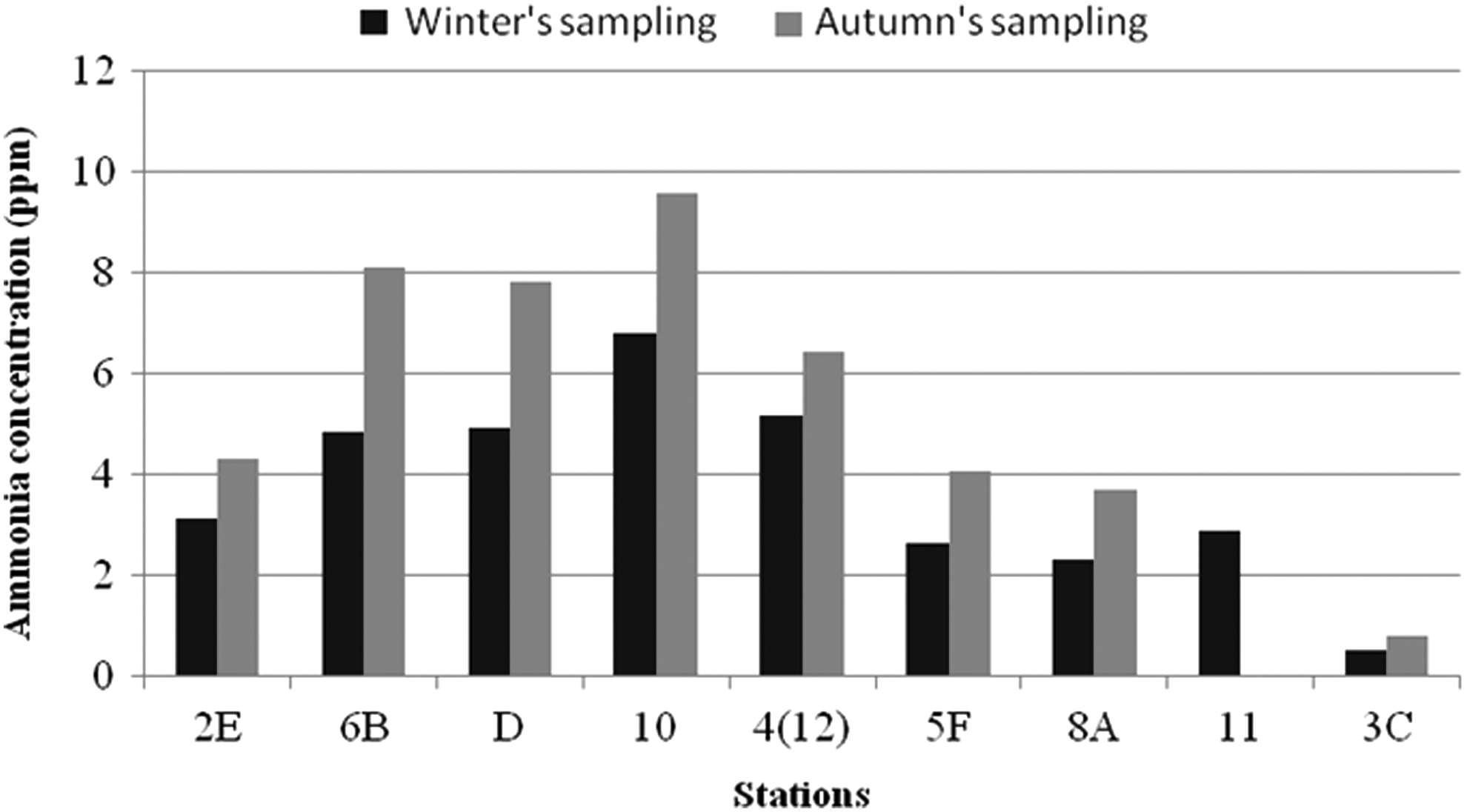
Detected ammonia concentrations at monitoring stations.

In the autumn, the ammonia emission rates from the composting facilities and landfill were around 1.143×10⁻³ and 2.007×10⁻⁴ g/m². Due to the areas of composting plant and landfill, area-integrated emission rates of ammonia were 134.80 and 96.73 g/s, respectively. In the winter, the ammonia emission of the composting plants and landfill was about 7.959×10⁻⁴ and 1.786×10⁻⁴ g/[m²·s], respectively. This means that the area-integrated emission rates of ammonia were 93.87 and 86.05 g/s (Fig. 3). As described in Figure 3, the ammonia emission rate of the composting plant was considerably higher than that of the landfill. In other words, the emission rates of composting plant in the autumn and winter are 5.67 and 4.4 times the corresponding values of the landfill, respectively. The comparison between ammonia emission rates in the autumn (at the temperature of 24°C) and winter (at the temperature of 4°C) depicted that a higher temperature increased the ammonia emission rate. This increase in the composting plant was more evident. The ammonia emission rate of the composting plant in the autumn was 1.43 times higher than the corresponding value in the winter. However, this difference for the landfill was about 1.12.

FIG. 3.

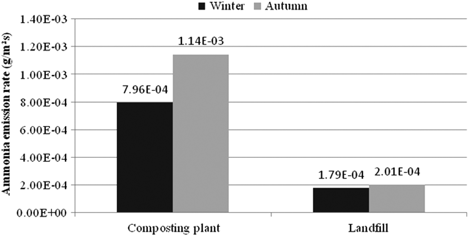
Predicted ammonia emission rate of Kahrizak composting plants and landfill.

As described in Equation (8), the wind speed has a prominent role in Lagrangian stochastic models. Therefore, any change in the direction and speed of wind may influence the estimations of ammonia emission rate. During ammonia sampling in the autumn season, the speed of wind varied between 2.2 and 3.5 m/s. This variation in the winter was between 2.2 and 2.7 m/s. Whether the temperature, air pressure, and direction of wind were constant, the prediction of the ammonia emission rate was approximately linearly related to wind speed (Figs. 4 and 5).

FIG. 4.

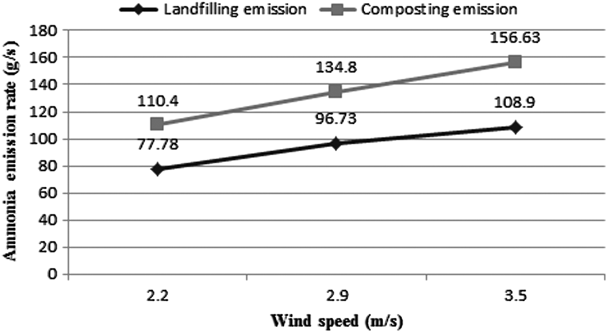
Ammonia emission rate at a different wind speed in autumn.

FIG. 5.

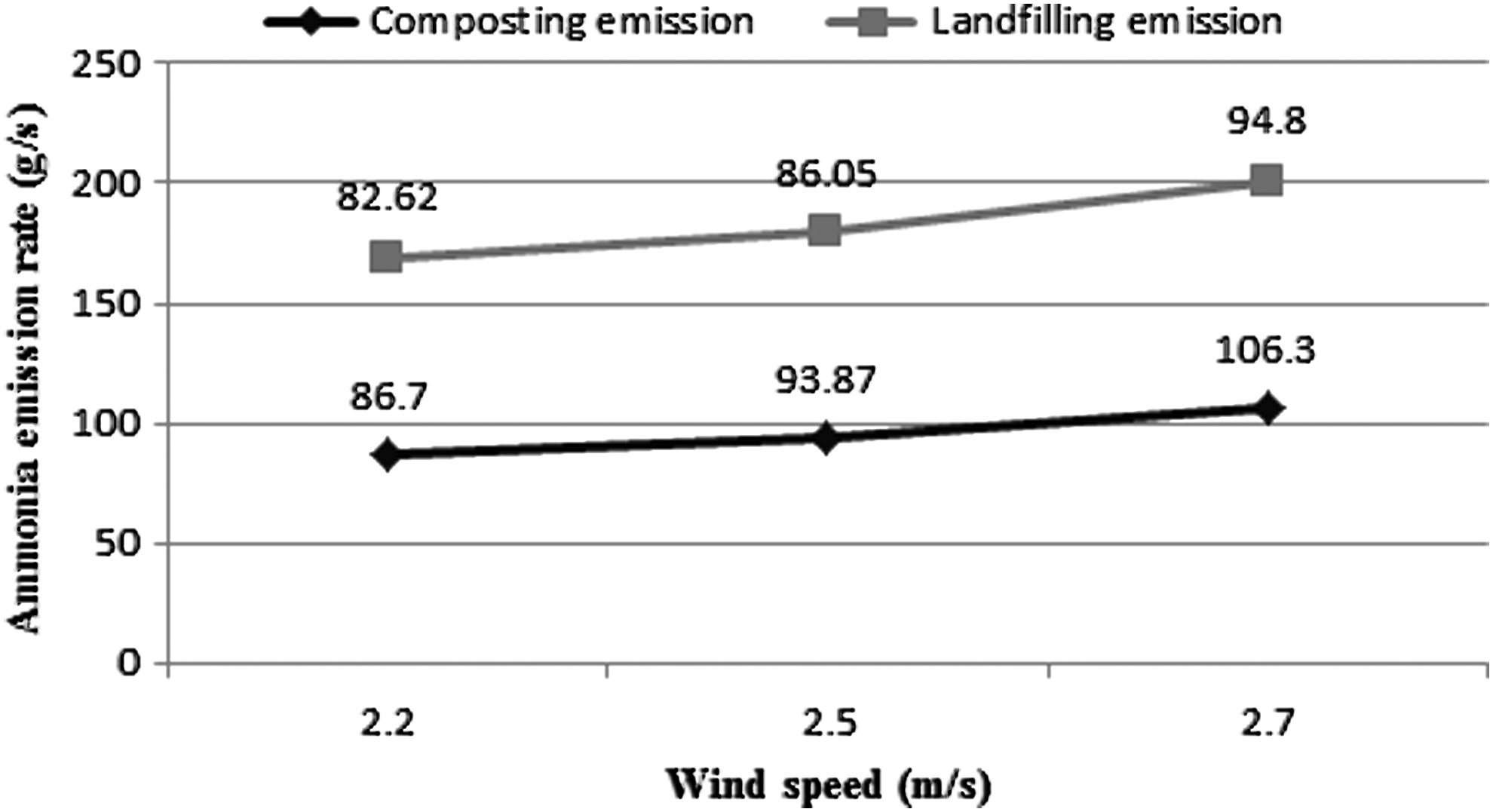
Ammonia emission rate at a different wind speed in winter.

A few studies about predicting ammonia emissions from full-scale composting processes have been carried out. Beck-Friss et al. (2001) studied the composting process in 200 L aerated reactors. They concluded that the ammonia emission rate of 1 ton organic fraction of MSW was 2.12 kg NH₃. Clemens and Cuhls (2003) reported that ammonia emissions in a composting process of an organic fraction of MSW for 1 ton of MSW are between 18 and 1,150 g. Cadena et al. (2009) attempted to determine gaseous emissions in a composting plant located in a Catalonia (Spain) treating source separated from MSW. They found in the aerated windrow composting process of 1 ton MSW that almost 3.9 kg ammonia was emitted into the atmosphere. The situation of the composting plants in the study area was similar to the study of Cadena et al. (2009). As previously mentioned, about 2,800 tons of Tehran's MSW were used for composting. Therefore, the daily ammonia emission rates in the autumn and winter from 1 ton MSW, which was processed in the aerated windrow composting, were 4.16 and 2.89 kg NH₃, respectively. Youssefi (2012) studied odor emission from Kahrizak landfill and composting facility. She indicated that ammonia emission from composting plants was around 103 g/s. However, in this study, ammonia emission in the autumn and winter was determined to be 134.80 and 93.87 g/s, respectively.

Due to the rate of biodegradability of solid waste in landfill, the total amount of gas produced for 1 kg MSW ranges from 0.87 to 1 m³, that is, for 1 pound of MSW the emitted gas varies between 14 and 16 ft³ (Tchobanoglous et al., 1993). One-tenth to one percent of the total released gases is ammonia (Tchobanoglous and Kreith, 2002). Four thousand tons per day of MSW are disposed off at the landfilling site, whose moisture content was assumed to be 25% by weight (Tchobanoglous and Kreith, 2002). Therefore, the dry mass of MSW in a landfill was 3,000 tons, which means that its ammonia emission rate could range from 0.0303 to 0.303 m³/s. In other words, in every second, the average ammonia released from the landfill varied between 23.4 and 234 g. Our results depicted that the emission of ammonia from the landfill in the autumn and winter was 96.73 and 86.05 g/s. Youssefi (2012) predicted the ammonia emission rate from Kahrizak landfill in January 6, 2008, using LandGEM-v302 software. She reported that the ammonia emission rate was 60 g/s, while the predicted ammonia emission in the winter (during December to January) was 86.05 g/s. This difference in the prediction of ammonia emission might be justified as follows:

• The locating of more monitoring stations at the Kahrizak landfill was not available.

• The characteristic of the MSW, which was disposed off in the landfill, was not considered in LandGEM software.

• The weather condition was not regarded in LandGEM software.

The comparison of our results with the studies mentioned earlier depicted a good convergence in predicting ammonia emission from the complex.

Prediction of the ammonia in the downwind

Due to the achieved results of the BLS technique in estimation of ammonia emission rate (ammonia considered an odorous compound), the downwind ammonia concentrations can be calculated using Screen View 3.5.0. We assumed the following assumptions to assess the autumn and winter downwind ammonia concentration:

• The SCREEN3 model is based on a single source (USEPA, 1995). As previously indicated, composting plants emitted the most ammonia at the site. Therefore, we selected the composting plant as the single source for using the software. The area source of the composting plant was 300×400 m.

• To account for the role of the landfill site in the ammonia emission, we added and distributed the total ammonia emission rate of the landfill on the composting plant dimensions. The emission rates of ammonia for landfill during the autumn and winter were calculated as 8.06×10⁻⁴ and 7.17×10⁻⁴ g/[m²·s], respectively [i.e., 7.17×10⁻⁴ g/[m²·s]=ratio of area integrated emission rate from the landfill (86.05 g/s) to the compost area dimension]. Therefore, we acquired the total emission rate of study area based on the dimensions of composting plants. In the autumn and winter, the total emission rates were 1.93×10⁻³ and 1.49×10⁻³ g/[m²·s], respectively.

• The mean directions of the wind in the autumn and winter were 285° and 135°, respectively.

• The study area was classified as a rural region.

The wind speed is one of the main factors in predicting the distances of ammonia dispersion [Equation (11)]. We ran the model for the minimum, mean, and maximum values of wind speed to identify the effect. The results of SCREEN3 dispersion model described that the variation of the wind speed did not have a significant effect on the ammonia concentration from distances more than 1,000 m from the source (Figs. 6 and 7). In addition, at an approximate distance of 1,800 m away from the source, the ammonia concentration would be negligible. The model results in the vicinity of the source did not have good agreement with the field measurement, as Zhu (1999) pointed out that Gaussian models (such as SCREEN3) prediction for distances less than 100 m from the source was not reliable. We had the limitation to measure ammonia concentration between zero distances and 450 m. However, the SCREEN3 predictions had relatively a good agreement with the field measurement (R²=0.85) when we move beyond the 450 m from the source. The standard deviations of the dispersion distance in the autumn and winter were around 44.73 m (ammonia concentration was 0.47 ppm) and 50.01 m (ammonia concentration was 0.47 ppm), respectively.

FIG. 6.

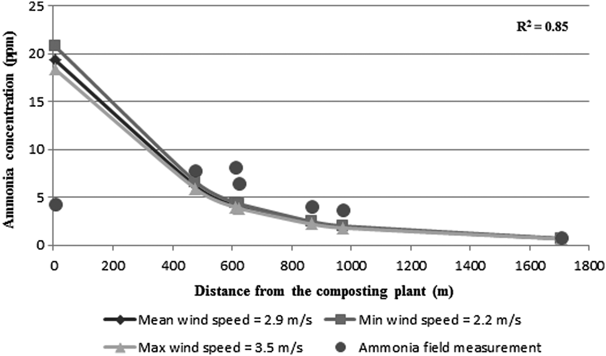
Difference between results of SCREEN3 model and field measurement in autumn.

FIG. 7.

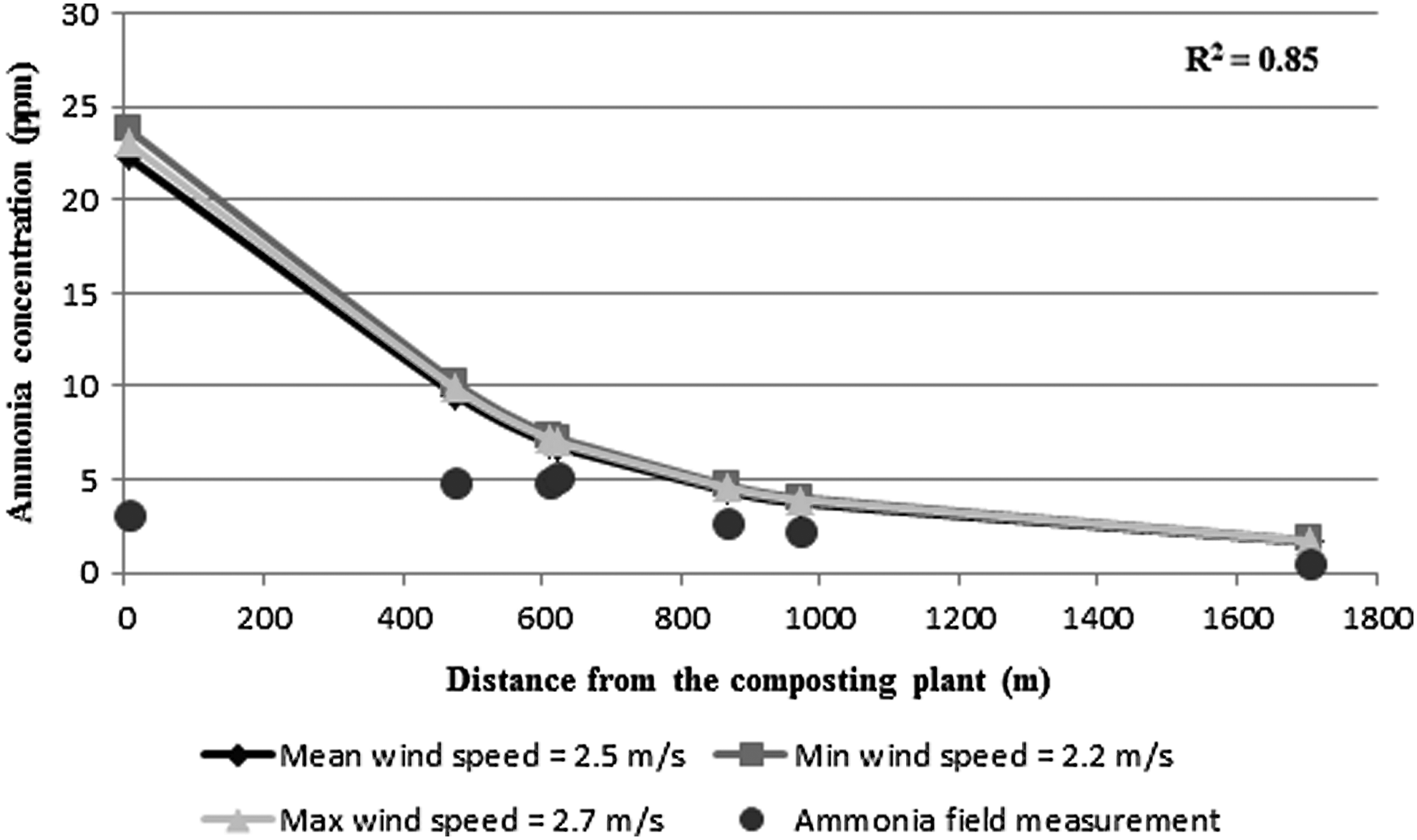
Difference between results of SCREEN3 model and field measurement in winter.

Youssefi (2012) predicted the emitted ammonia from Kahrizak landfill and composting facility using Environmental Protection Agency (EPA)'s ISC3 model. She estimated dispersion of ammonia for approximately 2,000 m away from the source. In her study, the average temperature, wind speed, and direction were considered 8.4°C, 3.6 m/s, and westerly, respectively.

Conclusions

Considering an experimental and mathematical study of Kahrizak composting plants and landfill, we summarized the following conclusions:

• Comparison of the monitored ammonia in each station indicated that the closer stations to the composting plants and landfill were more sensitive to the changes of temperature.

• The daily ammonia emission factors from the composting plants and landfill in the autumn were 4.16 and 2.02 kg/Mg of MSW, respectively. These values in the winter were predicted to be 2.89 and 1.86 kg/Mg of MSW.

• Due to the environmental features of the catchment area, the emitted ammonia could be detected for approximately 1,800 m away from Kahrizak landfill and composting plants. The result had good agreement with the field measurement.

• The results of the SCREEN3 model for the approximate distance less than 450 m from Kahrizak complex had a deep gap in comparison of the field measurement and could be considered unreliable.

• In addition, the results of the SCREEN3 model for the approximate distance more than 450 m from Kahrizak complex had a great convergence with the results of ammonia sampling (R²=0.85).

• Results depicted the good robustness of the BLS method in predicting ammonia emission rates from several sources and in contributing to the measured ambient concentration.

• Results of this study may be applicable to estimate ammonia emission rates in similar landfills and composting plants.

Footnotes

Acknowledgment

The authors would like to thank Arman Daneshikohan for his help in the preparation of this article.

Author Disclosure Statement

No competing financial interests exist.

References

Abdoli

, and Ghazizade

(2009). Comparison between anaerobic treatability of municipal landfill leachate containing both total and soluble substrate. J. Environ. Sci. Technol., 11, 61 (In Persian).

ASTM D1193 (2000). Specification for Reagent Water. West Cornshohocken, PA: ASTM International.

Beck-Friis

, Smars

, Jönsson

, and Kirchmann

. (2001). Gaseous emissions of carbon dioxide, ammonia and nitrous oxide from organic household waste in a compost reactor under different temperature regimes. J. Agric. Eng. Res., 78, 423.

Cadena

, Colón

, Sánchez

, Font

, and Artola

. (2009). A methodology to determine gaseous emissions in a composting plant. Waste Manag., 29, 2799.

Clemens

, and Cuhls

. (2003). Greenhouse gas emissions from mechanical and biological waste treatment of municipal waste. Environ. Technol., 24, 745.

Emerson

, Russo

R.C.

, Lund

R.E.

, and Thurston

R.V

. (1975). Aqueous ammonia equilibrium calculations: effect of pH and temperature. J. Fisheries Res. Board Canada, 32, 2379.

Flechard

C.R.

, Spirig

, Neftel

, and Ammann

. (2010). The annual ammonia budget of fertilised cut grassland—Part 2: seasonal variations and compensation point modeling. Biogeoscience, 7, 537.

Flesch

T.K.

, and Wilson

J.D.

(2005). Estimating tracer emissions with a backward Lagrangian stochastic technique. Agronomy Monograph No. 47. In Hatfield

J.L.

, Baker

J.M.

, and Viney

M.K.

, Eds., Micrometeorology in Agricultural Systems, Madison: American Society of Agronomy, Crop Science Society of America, and Soil Science Society of America, p. 513.

Flesch

T.K.

, Wilson

J.D.

, Harper

L.A.

, and Crenna

B.P

. (2005). Estimating gas emissions from a farm with an inverse-dispersion technique. Atmos. Environ., 39, 4863.

10.

Flesch

T.K.

, Wilson

J.D.

, Harper

L.A.

, Crenna

B.P.

, and Sharpe

R.R

. (2004). Deducing ground-to-air emissions from observed trace gas concentrations: a field trial. J. Appl. Meteorol., 43, 487.

11.

Flesch

T.K.

, Wilson

J.D.

, Harper

L.A.

, Todd

R.W.

, and Cole

N.A

. (2007). Determining ammonia emissions from a cattle feedlot with an inverse dispersion technique. Agric. Fores Meteorol., 144, 139.

12.

Flesch

T.K.

, Wilson

J.D.

, and Yee

. (1995). Backward-time Lagrangian stochastic dispersion models and their application to estimate gaseous emissions. J. Appl. Meteorol., 34, 1320.

13.

Harati

, Abdollahzade

, and Jamshidi

(2011). Investigating the potential for RDF production from reclaimed landfill in Iran (case study Arad Kooh landfill in Tehran), J. Environ. Sci. Technol., 13, 75 (In Persian).

14.

Holtslag

A.A.M.

, and Van Ulden

A.P

. (1983). A simple scheme for daytime estimates of the surface fluxes from routine weather data. J. Appl. Meteorol., 22, 517.

15.

Ivančič

, and Degobbis

. (1984). An optimal manual procedure for ammonia analysis in natural waters by the indophenol blue method. Water Res., 18, 1143.

16.

Lakes Environmental. (2013). Screen View™—Freeware, Onario, Canada. Available at: www.weblakes.com/products/screen/?AspxAutoDetectCookieSupport=1 (accessed December 12, 2013).

17.

Laubach

, and Kelliher

F.M

. (2005). Measuring methane emission rates of a dairy cow herd (II): results from a backward-Lagrangian stochastic model. Agric. Forest Meteorol., 129, 150.

18.

Liang

(2000). Nitrogen retention in the high rate stage of composting. PhD Dissertation, Department of Agricultural, Food and Nutritional Science, University of Alberta, Canada.

19.

Lodge

J.P.

(1989). Methods of Air Sampling and Analysis. 3rd Edn., Florida: Lewis Publisher.

20.

McGinn

S.M.

, Flesch

T.K.

, Crenna

B.P.

, Beauchemin

K.A.

, and Coates

. (2007). Quantifying ammonia emissions from a cattle feedlot using a dispersion model. J. Environ. Qual., 36, 1585.

21.

Oke

T.R.

(1978). Boundary Layer Climates. New York: John Wiley and Sons, Inc.

22.

Pagans

, Barrena

, Font

, and Sánchez

. (2006). Ammonia emissions from the composting of different organic wastes. Dependency on process temperature. Chemosphere, 62, 1534.

23.

Paine

R.J.

(1987). User's Guide to the CTDM Meteorological Preprocessor (METPRO) Program. EPA-600/8-88-004, U.S. Environmental Protection Agency, Research Triangle Park, NC. (NTIS No. BP 88-162102). Available at: http://cfpub.epa.gov/si/si_public_record_Report.cfm?dirEntryID=50449 (accessed August 10, 2013).

24.

Panofsky

H.A.

, and Dutton

J.A

. (1984). Atmospheric Turbulence: Models and Methods for Engineering Applications. New York: John Wiley and Sons, Inc.

25.

Richard

, Trautmann

(1996). The Science and Engineering of Composting. Cornell University. Available at: http://compost.css.cornell.edu/science.html (accessed October 10, 2013).

26.

Sawyer

C.N.

, McCarty

P.L.

, and Parkin

G.F

. (1994). Chemistry for Environmental Engineering. New York: McGraw-Hill Book Company.

27.

Skjøth

C.A.

, and Geels

. (2013). The effect of climate and climate change on ammonia emissions in Europe. Atmos. Chem. Phys., 13, 117.

28.

Sommer

S.G.

, McGinn

S.M.

, and Flesch

T.K

. (2005). Simple use of the backwards Lagrangian stochastic dispersion technique for measuring ammonia emission from small field-plots. Eur. J. Agron., 23, 1.

29.

Tchobanoglous

, and Kreith

. (2002). Handbook of Solid Waste Management. , 2nd edn, New York: McGraw-Hill, Inc..

30.

Tchobanoglous

, Theisen

, and Vigil

. (1993). Integrated Solid Waste Management: Engineering Principles and Management Issues. New York: McGraw-Hill, Inc..

31.

Tehran Municipality. (2013). Climate of Tehran, Tehran, Iran. Available at: http://en.tehran.ir/Default.aspx?tabid=106 (accessed October 10, 2013).

32.

Tehran Waste Management Organization (TWMO). (2008). Arad-Kouh Waste Disposal and Processing Complex. Available at: http://pasmand.tehran.ir/Default.aspx?tabid=90 (accessed October 10, 2013).

33.

Theobald

M.R.

, Løfstrøm

, Walker

, Andersen

H.V.

, Pedersen

, Vallejo

, and Sutton

M.A

. (2012). An intercomparison of models used to simulate the short-range atmospheric dispersion of agricultural ammonia emissions. Environ. Model. Softw., 37, 90.

34.

Thunder Beach Scientific. (2004). WindTrax Software, Nanaimo, Canada. Available at: www.thunderbeachscientific.com (accessed September 1, 2013).

35.

Todd

R.W.

, Cole

N.A.

, Clark

R.N.

, Flesch

T.K.

, Harper

L.A.

, and Baek

B.H

. (2008). Ammonia emissions from a beef cattle feedyard on the southern High Plains. Atmos. Environ., 42, 6797.

36.

US Environmental Protection Agency (USEPA). (1995). SCREEN3 Model User's Guide. EPA Publication No. EPA-454/B-95-004. Available at: www.epa.gov/scram001/userg/screen/screen3d.pdf (accessed August 1, 2013).

37.

US Environmental Protection Agency (USEPA). (2000). Meteorological Monitoring Guidance for Regulatory Modeling Applications. EPA-454/R-99-005. Available at: www.epa.gov/scram001/guidance/met/mmgrma.pdf (accessed August 5, 2013).

38.

Wark

(1995). Advanced Thermodynamics for Engine. ers, New York: McGraw-Hill.

39.

Webb

, and Misselbrook

T.H

. (2004). A mass-flow model of ammonia emissions from UK livestock production. Atmos. Environ., 38, 2163.

40.

Wyngaard

J.C.

(1988). Structure of the PBL. In: Venkatram

and Wyngaard

, Eds., Lectures on Air Pollution Modeling. Boston: American Meteorological Society, p. 9.

41.

Youssefi

(2012). Mathematical Model Development for Odor Emission from Kahrizak Landfill and Composting Plants Toward Residential Cities. MSc Thesis, Kharazmi University, Iran (In Persian).

42.

Zhang

(2008). Preventive Control of Ammonia and Odor Emissions During the Active Phase of Poultry Manure Composting. PhD Thesis, The University of British Columbia, Canada.

43.

Zhu

(1999). The influence of stability class on downwind odor concentration predicted by air dispersion models. J. Environ. Sci. Health Part A., 34, 1919.