Experimental Study of Electro-Kinetic Dewatering of Silt Based on the Electro-Osmotic Coefficient

Abstract

The electro-kinetic technique, which involves a direct electric current within porous media, has been studied extensively and applied in many areas. The technique is considered a promising method to dewater soil. However, uncertainty still exists as to the electro-osmotic coefficient, which is of great significance to the electro-kinetic dewatering effect. Therefore, the effective electro-osmotic coefficient and total electro-osmotic coefficient have been distinguished in this article. Influence of external factors (electric potential gradient, electrode material, and electrode spacing) and internal factors (initial water content, types of electrolytes, salt content, and humus content) on the electro-osmotic coefficient were investigated by laboratory experiments with Hangzhou silt. Results demonstrate that the external factors had a significant impact on the total coefficient but little influence on the effective coefficient. Internal factors such as initial water content, salt content, and humus content of the soil were found to have considerable impact on the effective coefficient whereas no obvious effect was noticed for varied electrolyte types. Moreover, critical values of the initial water content, salt content, and humus content were highlighted for the effective coefficient. The trend of the effective coefficient with a certain factor varies when the factor is within or beyond the critical value. As for the Hangzhou silt that was studied, critical values of the water content, salt content, and humus content were suggested to be between 70% and 79%, ∼0.5%, and between 10% and 20%, respectively. The electro-osmosis technique is believed to be inapplicable for soils with water content less than 70%, salinity higher than 2%, or humus content higher than 20%. The results obtained can provide guidance for evaluation of the applicability of the electro-osmosis technique.

Introduction

The electro-kinetic technique involves a direct electric current within porous media and has been studied extensively and applied in many areas, including soil stabilization (Cassagrande, 1949, 1983; Adamson et al., 1966; Shang, 1998; Burnotte et al., 2004), soil remediation (Jia et al., 2005; Ranjan and Manokararajah, 2005; Mena et al., 2016), and dehydration of wastewater sludge (Glendinning et al., 2008; Mahmoud et al., 2011; Tao et al., 2016). For soil stabilization, electro-osmosis, here referred to as the motion of water induced by the electro-kinetic technique, is considered a promising method for the treatment of soils with low permeability (Cassagrande, 1949, 1983; Bjerrum et al., 1967; Gray and Mitchell, 1967; Chappell and Burton, 1975; Mitchell, 1991; Shang et al., 2009).

Numerous researchers have reported the physical and chemical properties, such as soil water content or moisture content (Li, 2011; Tao et al., 2016), shear strength (Bergado et al., 2003; Shang et al., 2009; Tao et al., 2016), soil electric conductivity (Laursen, 1997; Bergado et al., 2003), Atterberg limits (Wu et al., 2016), zeta potential (Sumbarda-Ramos et al., 2010; Wu et al., 2016), and pH (Bergado et al., 2003; Estabragh et al., 2014) of soils stabilized by electro-osmosis. However, lack of understanding exists as to the soil electro-osmotic coefficient, which is a key parameter for the electro-kinetic dewatering process as the soil coefficient determines the ability of fluid to pass through the skeleton of the pores. Cassagrande (1949) studied the electro-osmotic coefficients of different soil types and found that the coefficients were quite steady with a value of ∼5E-5 cm²/sV. In this respect, Cassagrande (1949) regarded the electro-osmotic coefficient as one of the soil properties. This point of view was supported by Mitchell (1991). Since then, the electro-osmotic coefficient has been considered constant by a number of scholars, especially in theoretical and numerical studies (Cassagrande, 1949; Esrig, 1968; Su and Wang, 2003; Yuan et al., 2013). Nevertheless, other researchers have argued that the electro-osmotic coefficient is not constant and can be affected by many factors such as potential gradient (Lockhart, 1983a; Pang et al., 2011), void ratio (Feldkamp and Belhomme, 1990; Hu et al., 2012; Zhou et al., 2013), water content (Laursen, 1997), salinity (Li, 2011), pH (Lorenz and Philip, 1969), humic acid content (Chien et al., 2009), etc. For instance, Laursen (1997) found that the electro-osmotic coefficient increased with water content in the case of Ca bentonite and Na bentonite; Li (2011) studied the changes in the electro-osmotic coefficient with salinity in the range of 0–1.0% and found that k_e reached its peak when the salinity was 0.25%.

The electro-osmotic coefficient is of great significance in field experiments as well as in numerical simulation for the electro-osmosis technique. The electro-osmotic coefficient is one of the most important parameters for electro-osmosis calculation (Wan and Mitchell, 1976; Feldkamp and Belhomme, 1990; Su and Wang, 2003; Hu et al., 2012; Yuan and Hicks, 2016). However, disputes exist on the electro-osmotic permeability coefficient among previous scholars. To explore the influence of different factors on the electro-osmosis coefficient, a series of experiments with remolded soil was designed; two categories of the factors were highlighted, namely, external parameters and internal factors. The former category mainly consists of electrode material, potential gradient, and electrode spacing, and the latter includes water content, types of soluble salt, salt content, and humus content. These factors were investigated because they are common, accessible and can induce great impact on the electro-osmotic coefficient. Experimental results were interpreted from the total coefficient and the effective coefficient, which will be stated in detail in the next section. This study aimed at determining the influences of the concerned factor on the electro-osmotic coefficient and clarifying disputes in the preceding reports. The overall objectives of the study are to provide evaluation of the applicability of electro-osmosis as well as new perspectives to improve the electro-osmotic effect.

Effective Electro-Osmotic Coefficient and Total Electro-Osmotic Coefficient

Mathematically, the expression of the electro-osmotic coefficient is given as: \documentclass{aastex}\usepackage{amsbsy}\usepackage{amsfonts}\usepackage{amssymb}\usepackage{bm}\usepackage{mathrsfs}\usepackage{pifont}\usepackage{stmaryrd}\usepackage{textcomp}\usepackage{portland, xspace}\usepackage{amsmath, amsxtra}\usepackage{upgreek}\pagestyle{empty}\DeclareMathSizes{10}{9}{7}{6}\begin{document} \begin{align*} ke = \frac { v } { { ie } } = \frac { V } { A } { \frac { \Delta L } { \Delta \varphi } } , \tag { 1 } \end{align*} \end{document}

where v (cm/s) is the flow rate of the electro-osmotic flow in the soil; that is (V/cm) is the potential gradient, V (cm³) is the volume of electro-osmotic flow, A (cm²) is the cross-section area of the electro-osmotic flow, L (cm) is the seepage path, and Δφ is the potential difference across the soil samples. This article has distinguished between the effective electro-osmotic coefficient (k_ee) and the total electro-osmotic coefficient (k_e). The difference relies on the potential in calculation. In the electro-osmotic treatment, the output voltage from the power supply is not equal to the real voltage or the effective voltage applied on the soil since voltage loss exists between the electrodes and the soil, as discovered by Li (2011). When using the effective voltage in Equation (1), the electro-osmotic coefficient that is obtained is called the effective electro-osmotic coefficient, namely k_ee, \documentclass{aastex}\usepackage{amsbsy}\usepackage{amsfonts}\usepackage{amssymb}\usepackage{bm}\usepackage{mathrsfs}\usepackage{pifont}\usepackage{stmaryrd}\usepackage{textcomp}\usepackage{portland, xspace}\usepackage{amsmath, amsxtra}\usepackage{upgreek}\pagestyle{empty}\DeclareMathSizes{10}{9}{7}{6}\begin{document} \begin{align*} kee = \frac { V } { A } { \frac { \Delta L } { \Delta \varphi e } } \tag { 2 } \end{align*} \end{document}

Correspondingly, when using the total output voltage in calculation, the electro-osmotic coefficient is called the total electro-osmotic coefficient (k_e). In this study, the electro-osmotic coefficient has been thoroughly investigated from the perspective of the total coefficient as well as the effective coefficient. Attempts were also made to clarify the existing dispute regarding the electro-osmotic coefficient from these two perspectives.

Experimental Design

Samples and equipment

Undisturbed soil was collected in a foundation pit at Hangzhou, China and was divided into two parts (S₁ and S₂). The basic physical properties are given in Table 1. In the tests, the original soil was mixed with water to obtain moveable silts with a certain water content. The remolded soil was acquired as follows: (1) drying the undisturbed soil, grinding it into powder, putting it in a tray, pouring deionized water into the soil samples at the quality ratio of 1:5, and finally absorbing supernatant water with a straw until the soil samples changed into plain soil with a pH value of ∼7; (2) drying the plain soil in the oven; (3) grinding it and putting it into a mixing basin; (4) injecting water based on the target water content; (5) stirring the mixture to improve the uniformity, allowing the mixture to stand for 24 h, and finally testing the initial water content by the SL237-1999 test standard (Ministry of Water Resources of the People's Republic of China, 1999).

Table 1.

Basic Parameters of Undisturbed Soil

Serial no.	Density, g/cm ³	Specific gravity	Permeability coefficient, m/s	Water content, %	Saturation, %	Liquid limit, %	Plastic limit, %
S1	1.58	2.75	2.43 × 10⁻⁹	58.3	91.9	45.4	24.0
S2	1.61	2.73	2.27 × 10⁻⁹	41.5	93.1	37.2	17.2

The test equipment consists mainly of a self-made Miller box, DC power supply device, and water container. Two Miller boxes with the same design but different size, denoted as MA and MB, were used in this study and are shown in Fig. 1. MA and MB are made of plexiglass with the outer dimensions, respectively, 230 × 110 × 105 mm and 330 × 110 × 105 mm. Each box has two grooves with different size. The larger groove is used to accommodate soils and the smaller one to collect water. Two plate electrodes (with the dimensions of 100 × 100 × 4 mm) are attached to the two ends of the larger groove. On the cathodic plate, there are evenly perforated 5-mm diameter holes to drain. The cathode is wrapped with geotextile so that the water can be discharged through the geotextile filter and then flow to the beaker through the small hole in the smaller groove. To measure the effective potential in soil, three probes are inserted at the distance of 5 mm from the anode. The average of the measured results is taken as the anodic potential. The cathodic potential is obtained in the same way. Thus, the effective potential can be obtained by subtracting the anodic and cathodic potential (Mohamedelhassan and Shang, 2001; Li, 2011).

FIG. 1.

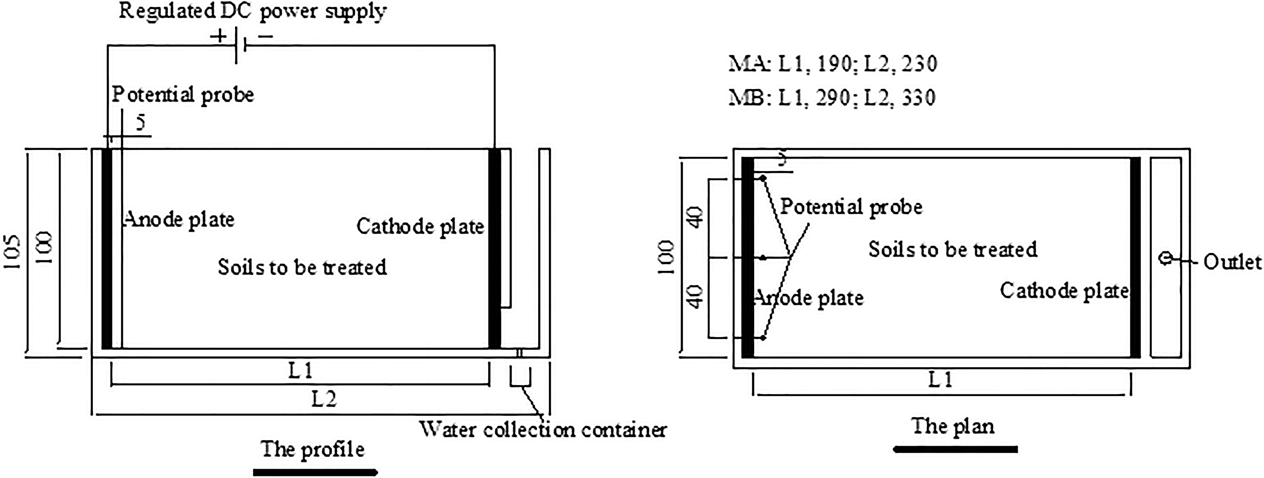
Diagram of Miller box MA and MB.

Experimental factors

For the external factors, Pang et al. (2011), Li (2011), and Wang et al. (2012) obtained a significant impact of the potential gradient and electrode spacing on the electro-osmotic coefficient, whereas huge disputes exist with their results. Moreover, electrode material is an important parameter in the electro-osmosis design. Therefore, electrode material, potential gradient, and electrode spacing were adopted as the external factors for the electro-osmotic coefficient. Specific evaluations of the external factors are given next.

Electrode material. Previous researchers performed many studies on electrode material, in which copper, iron, and aluminum electrodes were commonly used. Hence, these three materials were adopted in this study (Bjerrum et al., 1967; Lockhart, 1983b; Burnotte et al., 2004).

Potential gradient. A potential gradient range of 28–200 V/m was used in the existing literature (Lockhart, 1983a; Morris et al., 1985; Mohamedelhassan and Shang, 2001; Hu et al., 2012; Tao et al., 2016). Accordingly, potential gradients of 53, 79, and 158 V/m were employed in the experiments.

Electrode spacing. Distances of 190 and 290 mm were examined in these experiments, which were within the range of 100–400 mm tested by Li (2011).

As to the internal factors, initial water content, electrolyte type, salt content, and humus content were studied. Determinations of these factors are elaborated next.

Initial water content. The value of water content was set within the range of 50–80% according to the research of Laursen (1997).

Electrolyte type and salt content. To explore the impact of salt type and content on the electro-osmotic coefficient, inorganic electrolytes NaCl, Na₂CO₃, CaCl₂, and AlCl₃ were chosen in this study, due to their wide distribution in China. The results can also demonstrate the influence of anion and cation valences on the electro-osmotic process. Micic et al. (2001) performed an electro-osmosis test on Marine clay and found corrosion in the anode. Chew et al. (2004) used a conductive plastic drainage board in electro-osmosis treatment in an offshore reclamation project in Singapore, and the effect was not desirable. These results show that electro-osmosis is unsuitable for high-salinity-marine deposits. In addition, Mitchell (1991) expected good treatment effects for pore water salinity lower than 2 g NaCl/L, or soil electrical conductivity less than 0.25 S/m. Therefore, salinities of 0.25%, 0.5%, 1%, and 2% were used in this study. Here, the salinity refers to the mass percentage of salt contained in the dry soil (Li, 2011).

Humus content. The main humus species in natural soil are humic acid and fulvic acid (Shao et al., 2007), which are chemically stable and take approximately hundreds of years to decompose. Existing studies demonstrated that alkaline, dry, and aerobic conditions are beneficial to humic acid, whereas acidic, moist, and hypoxic conditions can promote the formation of fulvic acids. To simplify the experiment, the ratio of humic acid and fulvic acid was set as 1:1 to simulate the natural condition. Humic acid can be produced through biochemistry and mineralization. Normally, mineralized humic acid is obtained by extracting it from the soil. Thus, mineralized humic acid, more than the biochemistry acid, is similar to the actual soil. In this respect, mineralized humic acid was adopted in the tests. Nevertheless, a large difference exists with the humus contents in natural soils. Some soils have humus content less than 1%, whereas others, such as peat soil, have more than 20%. For the general cultivation layer, the humus content is within 3–5% (Shao et al., 2007). Therefore, the humus content was set as: 0%, 1%, 3%, 5%, 10%, and 20% in the tests.

In summary, influential factors for the electro-osmotic coefficient studied in this article, namely, external factors (potential gradient, electrode, and electrode spacing) and internal factors (water content, the type of electrolytes, salinity, and humus content) are listed in Tables 2 and 3.

Table 2.

External Factors for Electro-Osmotic Coefficient

Factors	Test no.	Electrode spacing, mm	Output voltage, V	Electrode material
Potential	A1	190	30	Copper
	A2		15
	A3		10
Electrode material	B1	190	15	Aluminum
	B2			Iron
	B3			Copper
Electrode spacing	C1	190	20	Iron
Electrode spacing	C2	290	30	Iron

Table 3.

Internal Factors for Electro-Osmotic Coefficient

Factors	Test no.	Initial water content, %	Electrolyte type	Salinity, %	Humus content, %
Initial water content	D1	51.1	—	—	—
	D2	57.5
	D3	69.8
	D4	79.4
Electrolyte type, salinity	E0	69.8	—	—
	E1	69.2	NaCl	0.25
	E2	70.2	Na₂CO₃
	E3	69.5	CaCl₂
	E4	70.1	AlCl₃
	E5	70.3	NaCl	0.5
	E6	69.8		1
	E7	71.0		2
Humus content	F0	69.8	—	—	0
	F1	69.7			1
	F2	68.3			3
	F3	70.1			5
	F4	69.6			10
	F5	70.3			20

Experimental procedure

The test started with making saturated-remolded soil samples, dissolving salt or humus in water, and stirring the mixture based on the target water content, salt content, or humus content. Then, the cathode was wrapped in geotextile, wet with water, put in the Miller box, and connected to the power. To eliminate the generation of bubbles, the soil samples were embedded in the Miller box by layers. An empty beaker was weighed and placed under the outlet of the smaller groove. Meanwhile, three probes were inserted near the anodic plate as well as the cathodic plate. Then, the circuit was connected and the output voltage was set. The power was turned on, and the electro-osmotic process began. During the process, the current, probe potentials, and the beaker weight were measured every hour to calculate the electro-osmotic coefficient and compare the electro-osmotic effect. Specifically, current values were recorded from the power supply. Probe potentials were measured with a digital voltmeter. Water discharges were computed from the difference of breaker weight. The process lasted for 29 h since volumes of effluent water for the last 3 h were all 1% lower than the corresponding total drainage. The tests ended by clearing away the soil and cleaning the equipment.

To explore the repeatability of the experiments, the electrode material tests were performed in triplicate. The experiment error was analyzed based on the monitored drainage. The ranges of the three data were within 15% of the average drainage at each moment. Therefore, the experimental errors were believed acceptable and the middle data of the tests for each electrode were adopted in this article. Moreover, the experiments were considered repeatable, and other tests were performed only once.

Experimental Results and Analysis

External factors for electro-osmotic coefficient

Potential gradient

Variations of the total electro-osmotic coefficient k_e with time for tests A1–A3 are shown in Fig. 2. The parameter k_e started from ∼7E-5 cm²/sV and ended with ∼1.5E-5 cm²/sV, with obvious difference of the three curves in the middle period. Therefore, the electro-osmotic process can be divided into three stages, namely stage I (0–12 h), stage II (12–26 h), and stage III (26–29 h). During stage I, k_e was relatively large and had obvious fluctuations yet declined rapidly. Nearly half of the total drainage occurred in stage I. During stage II, k_e decreased more slowly compared with stage I, yet faster than stage III. In stage III, k_e reached the minimum due to soil cracks and reduction of the soil water content. According to these three stages, designers can set different voltages during the electro-osmotic process to improve k_e as well as the electro-osmotic effect. Figure 2 also demonstrates that k_e decreased with increased potential gradient, especially in stage II. Similar results were also obtained by Pang et al. (2011), who considered that the total electro-osmotic coefficient is lower when the potential is higher. Mathematically from Equation (1), this lowering of the electro-osmotic coefficient occurred because the change rates of the electro-osmotic flow were smaller than that of the total potential.

FIG. 2.

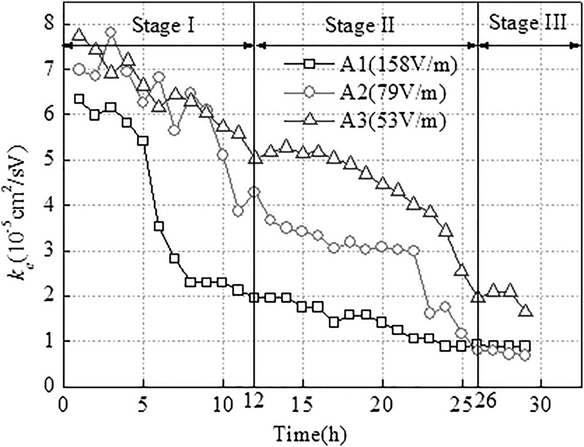
Total electro-osmotic coefficient k_e under different potential gradient.

The effective electro-osmotic coefficient was calculated by substituting the effective potential into Equation (2). The results are shown in Fig. 3. Similar to k_e in Fig. 2, k_ee also declined with time, from the initial value of ∼9E-5 to 4E-5 cm²/sV. However, the differences in the three curves were much less than in Fig. 2. For instance, the average difference of the total electro-osmotic coefficient was 2.63 whereas the average difference of the effective electro-osmotic coefficient was 1.46. Herein, the average difference refers to the average value of the differences of the maximum and minimum coefficient for A1–A3 every hour. Therefore, it is concluded that the total electro-osmotic coefficient is more dispersive. Moreover, k_ee is independent of the potential gradient whereas k_e can be substantially influenced by the potential gradient.

FIG. 3.

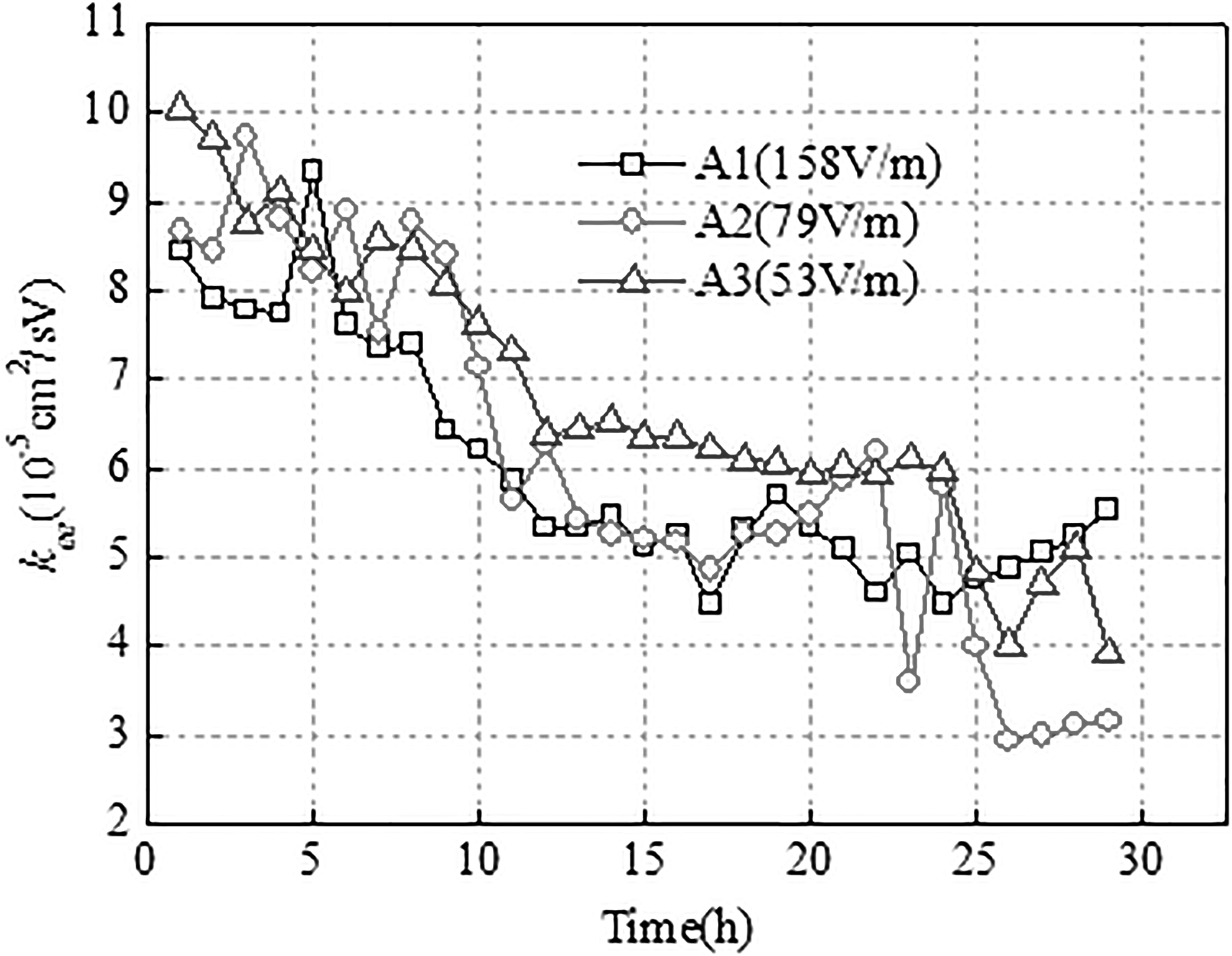
Effective electro-osmotic coefficient k_ee under different potential gradient.

The different results of the total and effective electro-osmotic coefficient come from the effective potential, which is the only difference in the formulas for the two coefficients. Figure 4 shows the curves of the effective potential for A1–A3. In the case of A1 (158 V/m), the effective potential was ∼25.8 V initially, then it dropped dramatically to only 14.5 V, followed by gradually decreasing until the end of the experiment. The initial rapid reduction of the curve for A1 is caused by electrochemical passivation of the copper anodes, as discussed by Zhou et al. (2015). For A2 (79 V/m), the initial effective potential was 12.33 V and then appeared to undergo a slow decline, which substantially coincided with A1. In the case of A3 (53 V/m), the effective potential was 7.70 V initially and stayed almost unchanged within the first 20 h. For the first 20 h of A3, the average effective potential was 7.76 V and the corresponding standard deviation was 0.24. Therefore, the effective potential loss was more obvious under higher voltage. Moreover, the effective potentials were close in stages II and III for A1–A3, even though the three tests were much different in total potential. With closer effective potentials, closer effective electro-osmotic coefficients were obtained from Equation (2). Thus, the total electro-osmotic coefficient displayed higher discreteness than the effective electro-osmotic coefficient. Further, the potential gradient was considered to have a great influence on the total electro-osmotic coefficient but little impact on the effective electro-osmotic coefficient.

FIG. 4.

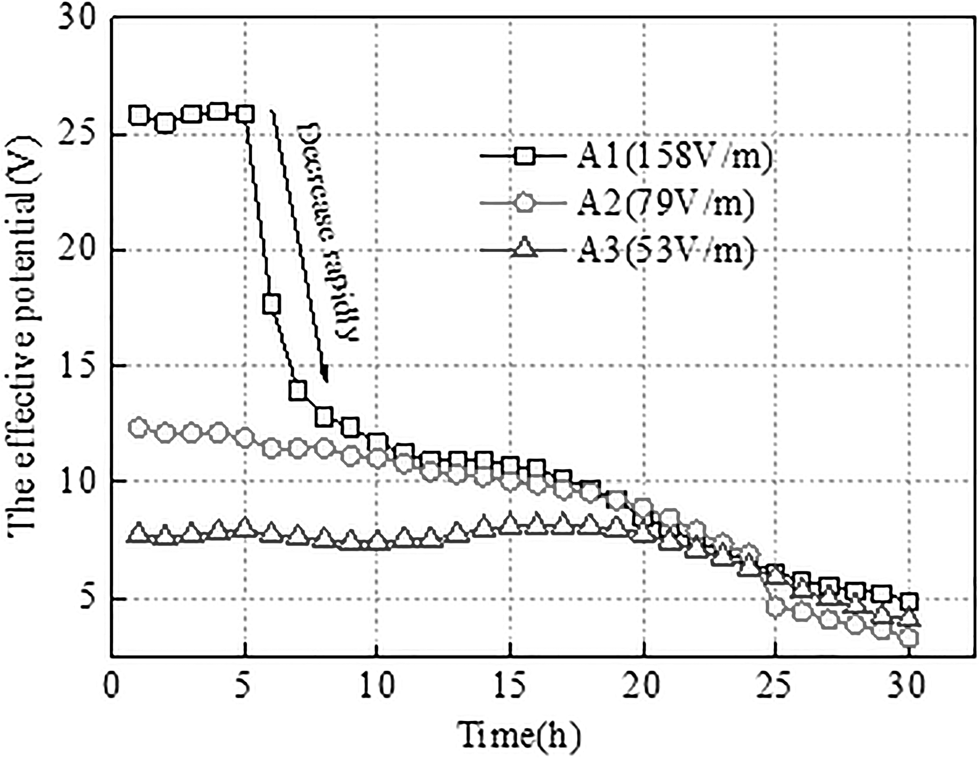
Effective potentials for tests A1–A3.

Electrode material

Figure 5 shows the total electro-osmotic coefficient obtained with different electrode materials. The total electro-osmotic coefficient k_e was smaller in the first 24 h for B1 (aluminum electrode), whereas k_e of B2 (copper electrode) and B3 (iron electrode) were quite close. Intersections were also discovered for B2 and B3. The smaller k_e of B1 can be caused by its smaller effective potential, which, according to Tao (2015), is mainly a result of the dense oxide film of aluminum leading to more soil-electrode interfacial resistance.

FIG. 5.

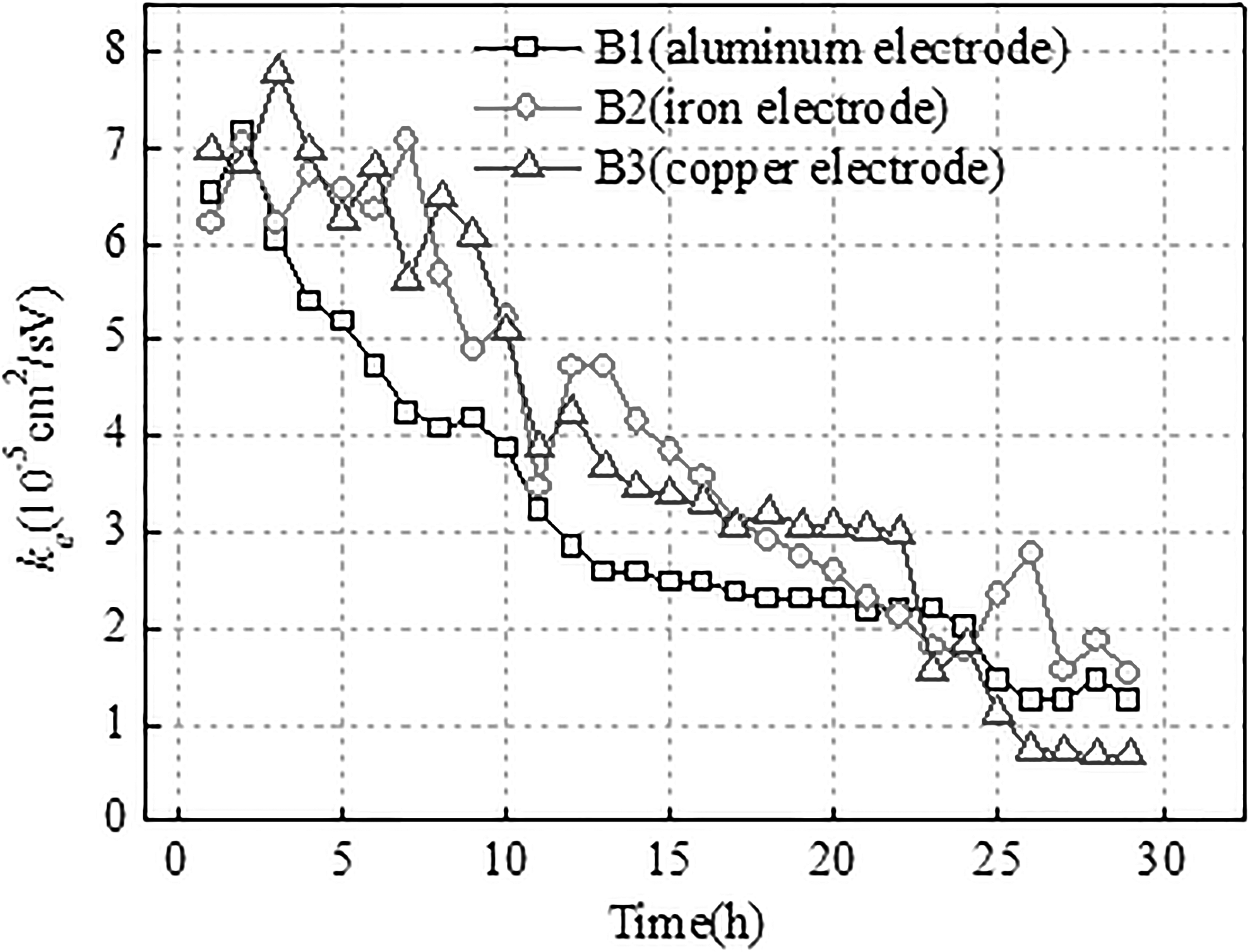
Total electro-osmotic coefficient k_e with different electrode materials.

Figure 6 displays the effective electro-osmotic coefficient of B1–B3. Figure 6 shows that the three curves were close. The average coefficient of B1, B2, and B3 is, respectively, 3.18, 3.99, and 3.88 cm²/sV, and the differential ratio between the maximum and the minimum is within 20%. Similar results were also obtained by Mohamedelhassan and Shang (2001). They studied the effective electro-osmotic coefficient of six different electrode groups. An average coefficient of 8.86–9.57 cm²/sV was achieved, with the differential ratio between the maximum and the minimum being within 7.4%. These results demonstrate the independence of k_ee of the electrode material.

FIG. 6.

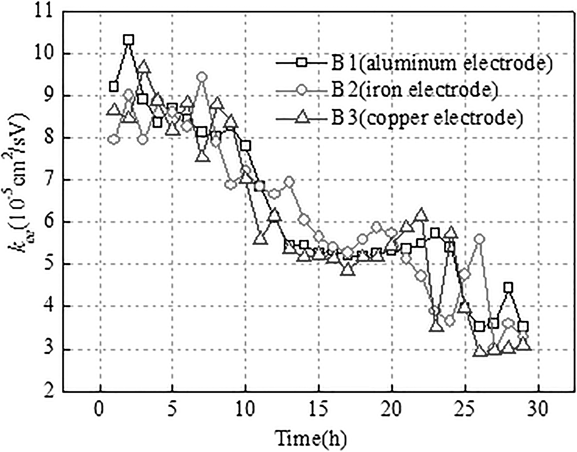
Effective electro-osmotic coefficient k_ee of different electrode materials.

Electrode spacing

Changes of k_e, k_ee and the effective potential with time for tests C1 and C2 are illustrated in Fig. 7. The effective potential gradient of C2 was relatively stable in the range of 0.91–0.95 V/cm, whereas C1 had a wider distribution of effective potential gradient in the range of 0.88–1.03 V/cm. Further, Fig. 7 presents very similar curves of k_e (or k_ee) for C1 and C2, revealing that electrode spacing was not a significant factor if the potential gradient was similar when using plate electrodes.

FIG. 7.

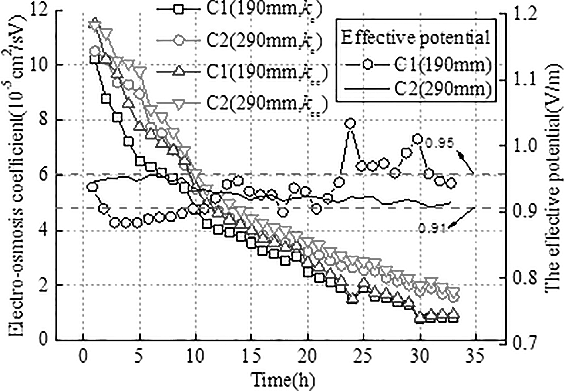
The k_e, k_ee and effective potential under different electrode spacing.

The earlier results show that the effective electro-osmotic coefficient was independent of the concerned external factors, whereas the total electro-osmotic coefficient was greatly influenced by external factors such as potential gradient and electrode material. No direct influence on the effective or total electro-osmotic coefficient was detected for electrode spacing.

Internal factors for electro-osmotic coefficient

Based on the conclusions in the external factors section, it is assumed that the effective electro-osmotic coefficient can be related to the internal factors such as soil water content, types of soluble salt, salt content, and humus content. Therefore, the effective electro-osmotic coefficient was investigated next, and the electro-osmotic coefficient in this section refers to the effective electro-osmotic coefficient (k_ee).

Water content

Figure 8 shows the effective electro-osmotic coefficient k_ee under varied initial water content. The average k_ee in the first 10 h, the maximum and the minimum k_ee are presented to illustrate the experimental results clearly. The average k_ee in the first 10 h is adopted as a reasonable reflection for the effect of the initial water content on k_ee as the soil water content changes with the electro-osmotic process. Figure 8 shows that the maximum and average k_ee increase with water content whereas the minimum k_ee decreases slightly. The average of k_ee increases from 4.55 × 10^–5 to 8.13 × 10^–5 cm²/sV with water content growing from 51.1% to 69.8%. The maximum k_ee also increases, yet with a decreasing rate.

FIG. 8.

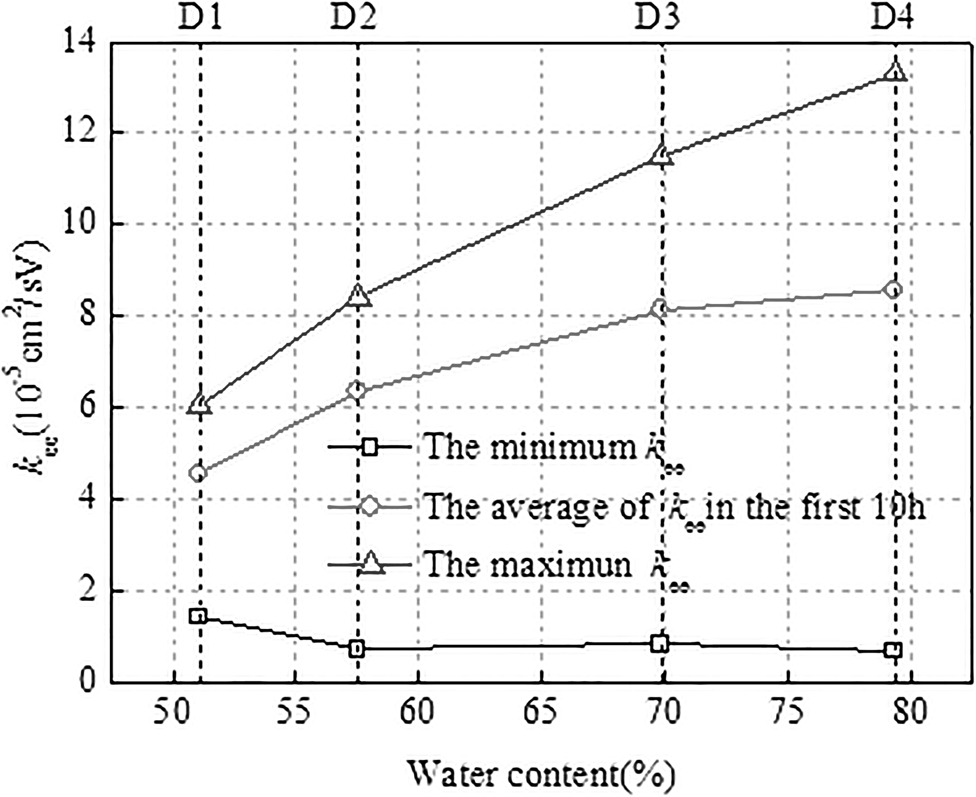
Effective electro-osmotic coefficient versus initial water content.

The total drainage of D1, D2, D3, and D4 is, respectively 215.70, 346.40, 464.17, and 461.10 mL. Drainages of D3 (69.8%) and D4 (79.4%) are similar with less than 1% difference, which also gives the upper limit of the drainage. With respect to the effective potential, similar data for D3 and D4 were also obtained in the tests. Therefore, the drainage and effective potential barely changes with the initial water content increasing from 69.8% to 79.4%. It can be further deduced that k_ee will vary little with the water content range of 69.8–79.4% based on Equation (1). In this respect, marginal initial water content exists from the perspective of the electro-osmotic coefficient. In other words, k_ee will increase with water content below the critical value, and it will maintain or decrease when water content is above the critical value. For the concerned Hangzhou silt, the marginal moisture content is considered within 70–79%.

Salt content

Figure 9 shows the effective electro-osmotic coefficient k_ee under varied salt content. Similarly, the average k_ee in the first 4 and 10 h, the maximum and the minimum k_ee are presented to illustrate the experimental results clearly. E7 (salinity, 2%) is implied to possess the highest salt content but the lowest k_ee. This result is in accordance with that depicted by previous scholars (Micic et al., 2001; Chew et al., 2004). Mitchell (1991) pointed out that the electro-osmosis technique had better performance than other foundation treatment methods such as loading or vacuum preloading, when the salinity was less than 2 g/L or electrical conductivity did not exceed 0.25 s/m. Therefore, soil salt content has a significant impact on the electro-osmotic performance as well as the electro-osmotic coefficient.

FIG. 9.

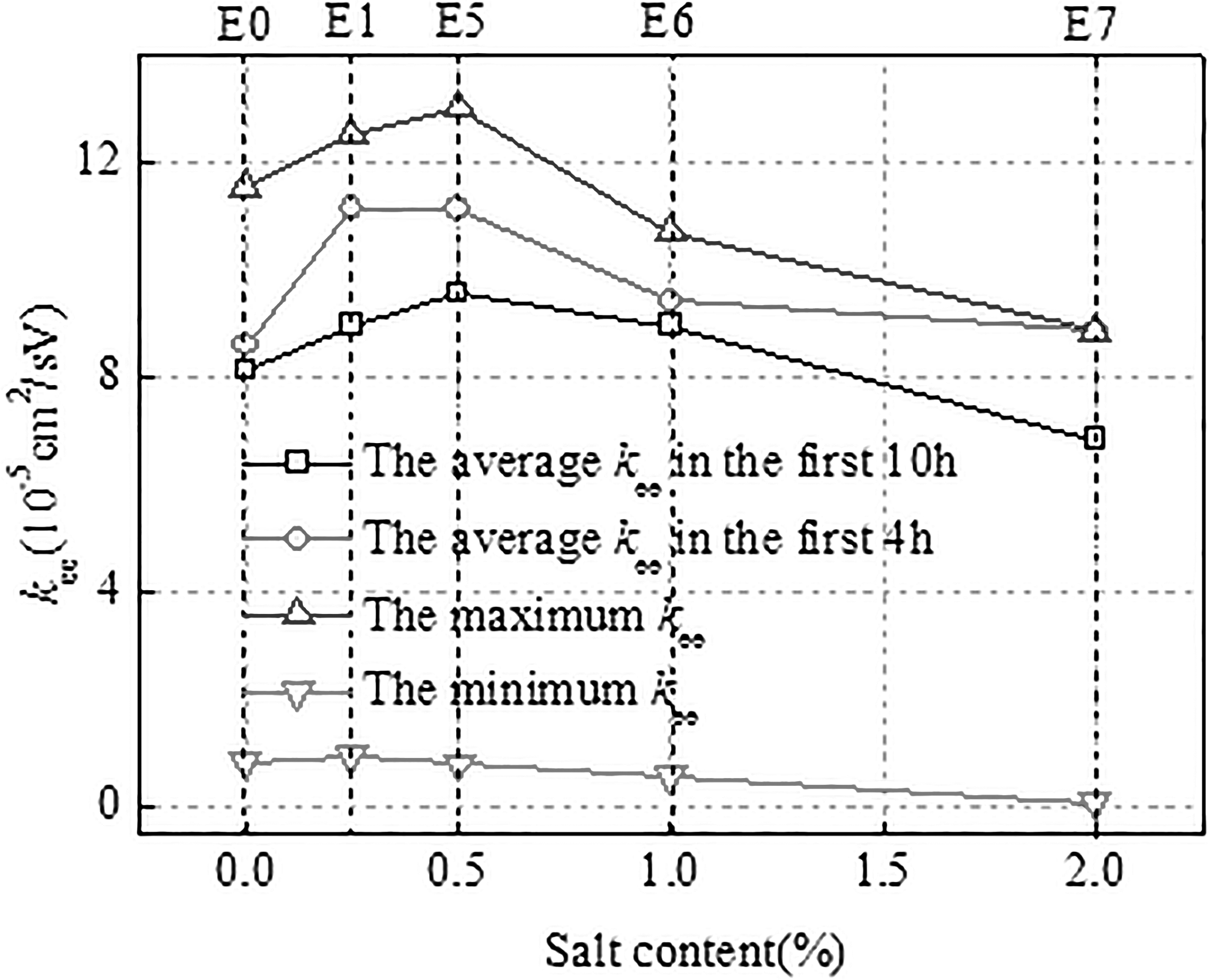
Effective electro-osmotic coefficient under different salt content.

Comparing the effective electro-osmotic coefficients k_ee under different salinity, Fig. 9 displays that the salinity of 0.5% corresponded to peak values of the maximum k_ee, the 4 h-average k_ee, and the 10 h-average k_ee, which were, respectively, 9.5E-5, 11.1E-5, and 13.0E-5 cm²/sV. More specifically, the maximum k_ee as well as the average k_ee in the first 4 and 10 h rose with salinity when the salinity was below 0.5% while displaying an opposite trend when the salinity was beyond 0.5%. This demonstrates the existence of the optimal salinity, which corresponds to the highest k_ee and the best electro-osmotic performance. Further discussion will be presented in the Discussion section.

Electrolyte types

Figure 10 illustrates the electro-osmotic coefficient k_ee with different electrolytes. To have a comprehensive investigation, the average k_ee in the first 4 and 10 h, the maximum and the minimum k_ee, and experimental results from Chien et al. (2009) are adopted in Fig. 10. The average k_ee in the first 10 h ranged from 7.93E-5 to 8.95E-5 cm²/sV, with the difference being 12.86%. The average k_ee in the first 4 h and the maximum k_ee are, respectively, 8.17E-5–10.3E-5 cm²/sV and 9.4E-5–13.5E-5 cm²/sV. To further explore these data for k_ee, statistical tests were performed. p-Values of E1–E2, E2–E3, E3–E4, and E4–T0 are 0.33, 0.43, 0.40, and 0.38, respectively. No significant difference was observed with different electrolytes. Therefore, it is deduced that different ions had little effect on the electro-osmotic coefficient in the case of 0.25% salt content.

FIG. 10.

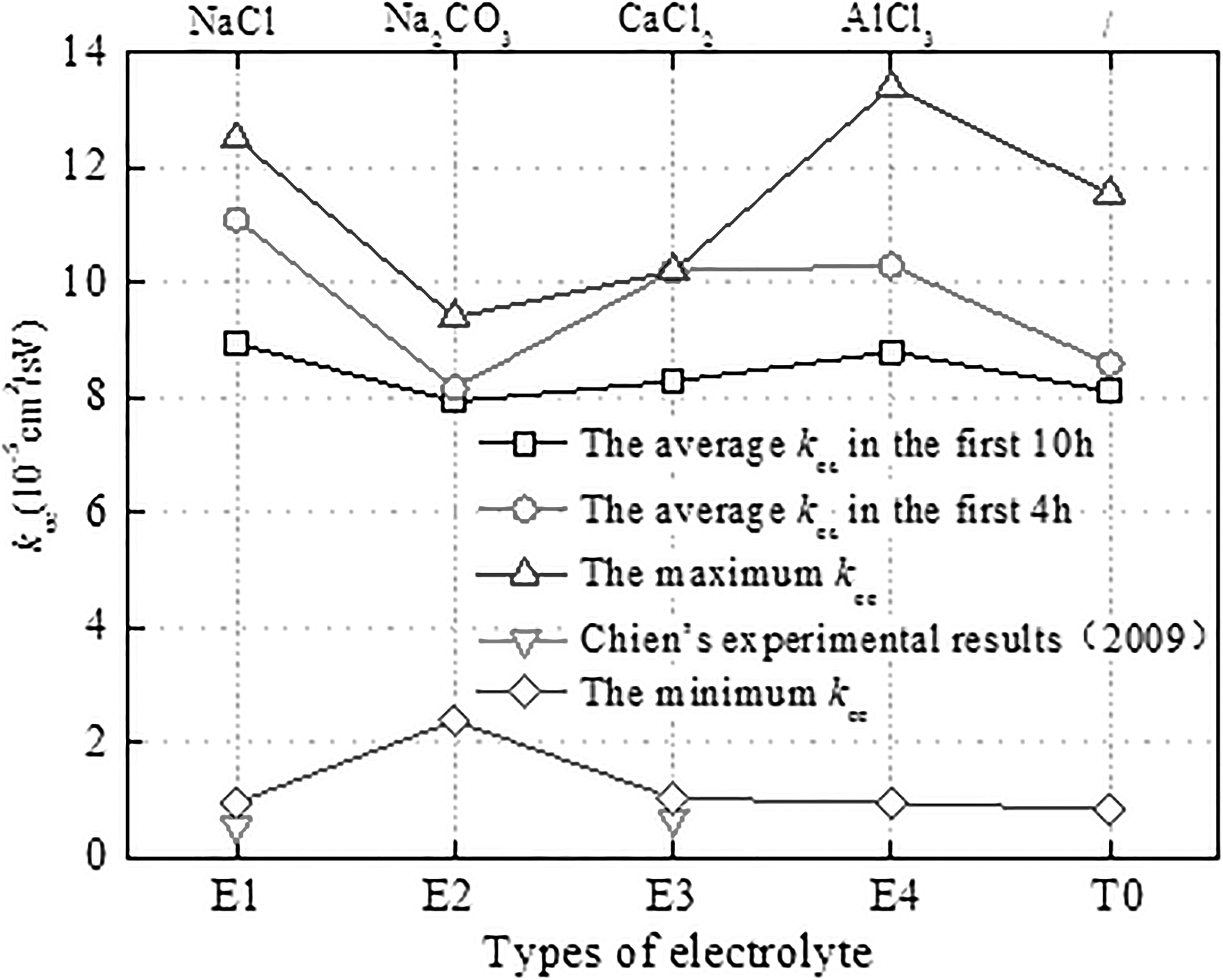
Effective electro-osmotic coefficient with different electrolytes.

Humus content

Figure 11 shows the development of the electro-osmotic coefficient k_ee with time under different humus content. The curves, except F5 (20%), were very close to each other in the first 20 h, with F2 (3%) and F3 (5%) being relatively higher. For F5 (20%), there was no significant difference from the other curves in the beginning. However, the curve of F5 (20%) declined substantially at ∼7 h and then stayed the lowest. This effect can be caused by the high acid content of F5, namely 20%. On the whole, similar developing trends of k_ee were obtained with humus content below 10%.

FIG. 11.

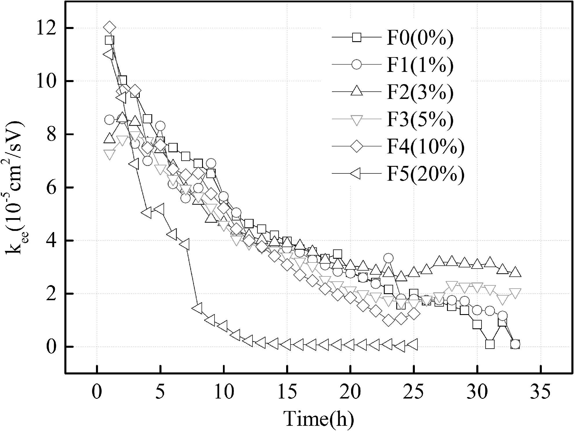
Effective electro-osmotic coefficient versus time under different humus content.

Figure 12 presents the average k_ee in the first 10 h with different humus content. The average k_ee ranged from 6.53E-5 (F3) to 8.11E-5 cm²/sV (F0) when the humus content was within 0–10%. Nevertheless, when the humus content ranged from 10% to 20%, the average k_ee decreased from 7.71E-5 to 4.88E-5 cm²/sV, with a rate of decrease of 37%. Combined with the consequences just mentioned based on Fig. 11, the humus content has significant influence on the electro-osmotic coefficient provided that the acid content exceeds some certain value, for instance 10% in our case.

FIG. 12.

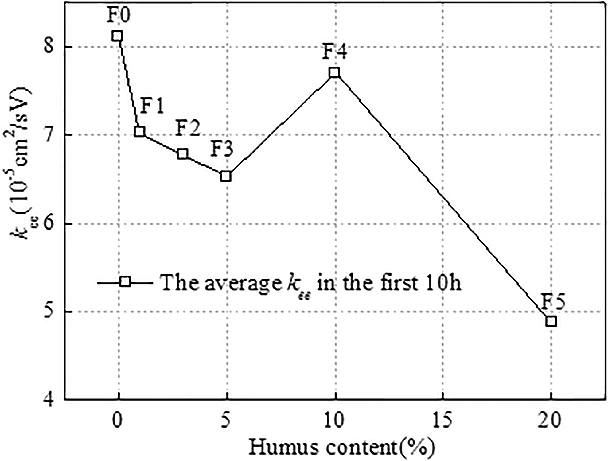
Average k_ee versus different humus content.

Discussion

External factors

For the external factors, there were obvious differences in the total electro-osmotic coefficient k_e when different potential gradient or electrode material was applied, whereas no obvious difference was observed for the effective electro-osmotic coefficient k_ee. The total electro-osmotic coefficient k_e decreased with increased potential gradient and electrode material affects k_e via effective potential or potential loss (Zhou et al., 2015). Thus, it is concluded that external factors such as potential gradient or electrode material possess significant effects on k_e. k_ee is believed to be independent of the external factors and is essentially a property of the soil, which is in accordance with Cassagrande (1949).

Internal factors

To sum up the internal factors, the average electro-osmotic coefficient k_ee in the first 10 h was taken for analysis. When the initial water content varied from 51% to 70%, the average k_ee increased with the water content. For salinity less than 0.5%, the average k_ee increased with salinity, whereas an opposite trend was attained with salinity higher than 0.5%. Obvious variation of the average k_ee was also attained when the humus content increased from 10% to 20%. It is, thus, concluded that the initial water content, soil salinity, and humus content exert a significant impact on the effective electro-osmotic coefficient. Moreover, critical values of the initial water content, salt content, and humus content were obtained for k_ee. For the adopted Hangzhou silt, critical values of the water content were suggested to be between 70% and 79%, humus content between 10% and 20%, and salt content ∼0.5%. Therefore, the electro-osmosis technique is not applicable for soils with water content less than 70%, salinity higher than 2%, or humus content higher than 20%. However, the type of electrolyte was found to have little influence on the average electro-osmotic coefficient. The largest difference of the k_ee was 12.86% for different soluble salts with the salinity of 0.25% because different ions have similar contributions to the transportation process of electro-osmosis (Zhou et al., 2015).

Remarkably, the pH value of Na₂CO₃ and AlCl₃ solution was, respectively, 11.4 and 3.6, whereas the average k_ee values in the first 10 h for E2 (Na₂CO₃) and E4 (AlCl₃) were 7.93E-5 and 8.80E-5 cm²/sV, with the difference being 10.97%. Hamed and Bhadra (1997) conducted two series of electrokinetic experiments on kaolinite to study the effects of influent pH on the electro-kinetic process and concluded that increasing the influent pH did not lead to any increase in the electric potential across the cell. Combined with our study, no significant impact of pH on the electro-osmotic coefficient was observed. However, other researchers obtained contradictory results. Lorenz and Philip (1969) and Xiang and Somasundaran (1996) determined the relationship between pH and zeta potential, based on which opposite zeta potentials will be deduced for pH 11.4 and 3.6. According to the Helmholtz–Smoluchowski theory, which gives the direct proportion of the electro-osmotic coefficient with zeta potential, electro-osmotic coefficients of soils with pH 11.4 will be opposite to those of soils with pH 3.6, indicating that the electro-osmotic flow will be in the opposite direction. Therefore, a great discrepancy exists between this research and previous studies (Lorenz and Philip, 1969; Xiang and Somasundaran, 1996). This discrepancy is caused by the constraints of the Helmholtz–Smoluchowski theory, which has overestimated the flow driving force and underestimated the flow resistance. Further studies need to be performed in this respect.

Conclusions

Laboratory experiments were performed to investigate the influence of three external factors (potential gradient, electrode materials, and electrode spacing) and four internal factors (water content, electrolyte type, salt content, and humus content) on the electro-osmotic coefficient. The results were presented in terms of the total and effective electro-osmotic coefficient. The effective electro-osmotic coefficient was found to be independent of the external factors. However, the total electro-osmotic coefficient was significantly influenced by external factors such as potential gradient and electrode material other than the electrode spacing. For the internal factors, the initial water content, soil salt content, and humus content were found to exert a significant impact on the electro-osmotic coefficient, whereas no obvious influence was observed with respect to electrolyte type.

It is also observed that the effective electro-osmotic coefficient increased with water content when the initial water content was below a certain value, while maintaining or decreasing when the water content was above this value. Similar results were also reported for salt content and humus content. Therefore, critical values of the initial water content, salt content, and humus content were emphasized for the effective electro-osmotic coefficient. In terms of the concerned Hangzhou silt, critical values of the water content and humus content were suggested to be between 70% and 79% and 10% and 20%, respectively, whereas the critical value of salt content was ∼0.5%. The electro-osmosis technique is considered to be inapplicable for soils with water content less than 70%, salinity higher than 2%, or humus content higher than 20%.

Footnotes

Acknowledgments

The study presented in this article was substantially supported by the Natural Science Foundation of China (grant nos. 51478425, 51708507, 41572299, 41602308), the National Key Research and Development Plan of China (grant no. 2016YFC0800203), the Natural Science Foundation of Zhejiang Province (grant nos. LQ17E090001, LZ13D020001), and the Open Fund of the MOE Key Laboratory of Soft Soils and Geoenvironmental Engineering (grant no. 2016P01).

Author Disclosure Statement

No competing financial interests exist.

References

Adamson

L.G.

, Chilingar

G.V.

, Beeson

C.M.

, and Armstrong

R.A.

(1966). Electrokinetic dewatering, consolidation and stabilization of soils. Eng. Geol. 1, 291.

Bergado

D.T.

, Sasanakul

, and Horpibulsuk

(2003). Electro-osmotic consolidation of soft bangkok clay using copper and carbon electrodes with pvd. Geotech. Test. J. 26, 277.

Bjerrum

, Moum

, and Eide

(1967). Application of electro-osmosis to a foundation problem in a Norwegian quick clay. Geotechnique, 17, 214.

Burnotte

, Lefebvre

, and Grondin

(2004). A case record of electroosmotic consolidation of soft clay with improved soil electrode contact. Can. Geotechn. J. 41, 1038.

Cassagrande

(1949). Electro-osmosis in soils. Géotechnique, 1, 159.

Cassagrande

(1983). Stabilization of soils by means of electro-osmosis: State of the art. J. Boston Soc. Civil Eng. 69, 255.

Chappell

B.A.

, and Burton

P.L.

(1975). Electro-osmosis applied to unstable embankment. J. Geotechn. Eng. Div. 101, 733.

Chien

S.C.

, Ou

C.Y.

, and Wang

M.K.

(2009). Injection of saline solutions to improve the electro-osmotic pressure and consolidation of foundation soil. Appl. Clay Sci. 44(3): 218.

Chew

S.H.

, Karunaratne

G.P.

, Kuma

V.M.

, Lim

L.H.

, Toh

M.L.

, and Hee

A.M.

(2004). A field trial for soft clay consolidation using electric vertical drains. Geotext. Geomembr. 22(12): 17.

10.

Esrig

M.I.

(1968). Pore pressure, consolidation, and electrokinetic. J. Soil Mech. Found. Div. 94, 899.

11.

Estabragh

A.R.

, Naseh

, and Javadi

A.A.

(2014). Improvement of clay soil by electro-osmosis technique. Appl. Clay Sci. 95, 32.

12.

Feldkamp

J.R.

, and Belhomme

G.M.

(1990). Large-strain electrokinetic consolidation: Theory and experiment in one dimension. Geotechnique, 40, 557.

13.

Glendinning

, Lamont-Black

, Jones

C.J.F

.P., and Hall

(2008). Treatment of lagooned sewage sludge in situ using electrokinetic geosynthetics. Geosynth. Int. 15, 192.

14.

Gray

D.H.

, and Mitchell

J.K.

(1967). Fundamental aspects of electro-osmosis in soils. J. Soil Mech. Found. Div. 93, 209.

15.

Hamed

J.T.

, and Bhadra

(1997). Influence of current density and pH on electrokinetics. J. Hazard. Mater. 55, 279.

16.

L.M.

, Wu

W.L.

, and Wu

(2012). Numerical model of electro-osmotic consolidation in clay. Géotechnique, 62, 537.

17.

Jia

, Larson

, Slack

, and Walworth

(2005). Electrokinetic control of nitrate movement in soil. Eng. Geol. 77, 273.

18.

Laursen

(1997). Laboratory investigation of electroosmosis in bentonites and natural clays. Can. Geotechn. J. 34, 664.

19.

(2011). Experimental and theoretic study on electro-osmotic consolidation of soft clay foundation. PhD thesis, Zhejiang University, Zhejiang.

20.

Lockhart

N.C.

(1983a). Electroosmotic dewatering of clays. I. Influence of voltage. Colloids Surf., 6, 229.

21.

Lockhart

N.C.

(1983b). Electroosmotic dewatering of clays, III. Influence of clay type, exchangeable cations and electrode materials. Colloids Surf., 6, 253.

22.

Lorenz

, and Philip

(1969). Surface conductance and electrokinetic properties of kaolinite beds. Clays Clay Miner. 17, 223.

23.

Mahmoud

, Olivier

, Vaxelaire

, and Hoadley

(2011). Electro-dewatering of wastewater sludge: Influence of the operating conditions and their interactions effects. Water Res. 45, 2795.

24.

Mena

, Villaseñor

, Rodrigo

M.A.

, and Cañizares

(2016). Electrokinetic remediation of soil polluted with insoluble organics using biological permeable reactive barriers: effect of periodic polarity reversal and voltage gradient. Chem. Eng. J. 299, 30.

25.

Micic

, Shang

J.Q.

, Lo

K.Y.

, Lee

Y.N.

, and Lee

S.W.

(2001). Electrokinetic strengthening of a marine sediment using intermittent current. Can. Geotechn. J. 38, 287.

26.

Mohamedelhassan

, and Shang

J.Q.

(2001). Effects of electrode materials and current intermittence in electro-osmosis. Proc. Inst Civil Eng. Ground Improv. 5, 3.

27.

Ministry of Water Resources of the People's Republic of China. (1999). Specification of soil test. SL237-1999.

28.

Mitchell

J.K.

(1991). Conduction phenomena: From theory to geotechnical practice. Geotechnique, 41, 299.

29.

Morris

D.V.

, Hillis

S.F.

, and Caldwellg

J.A.

(1985). Improvement of sensitive silty clay by electroosmosis. Can. Geotechn. J. 25, 17.

30.

Pang

, Liu

S.H.

, and Wu

. (2011). Lab experimental study on electro-osmotic parameters for soft soil consolidation. Port Water Eng. 148.

31.

Ranjan

R.S.

, and Manokararajah

(2005). Electrokinetic retention, migration and remediation of nitrates in silty loam soil under hydraulic gradients. Eng. Geol. 77, 263.

32.

Shang

J.Q.

(1998). Electroosmosis-enhanced preloading consolidation via vertical drains. Can. Geotechn. J. 35, 491.

33.

Shang

J.Q.

, Tang

Q.H.

, and Xu

Y.Q.

(2009). Consolidation of marine clay using electrical vertical drains. Geomech. Eng. 1, 275.

34.

Shao

Y.F.

, Gong

X.N.

, Xu

R.Q.

, and Liu

Z.Y.

(2007). Experimental study on stabilization of humus-containing soft soil. J. Zhejiang Univ. Eng. Sci. 41, 1472.

35.

J.Q.

, and Wang

(2003). The two-dimensional consolidation theory of electro-osmosis. Geotechnique, 53, 759.

36.

Sumbarda-Ramos

E.G.

, Guerrero-Gutierrez

O.X.

, Murillo-Rivera

, and Gonzalez

(2010). Electrokinetic treatment for clayed and sandy soils. J. Appl. Electrochem. 40, 1255.

37.

Tao

Y.L.

(2015). Electro-osmotic process under different electrode materials and a novel method for discharge calculation based on electrical conductivity. PhD thesis, Zhejiang University, Zhejiang.

38.

Tao

Y.L.

, Zhou

, Gong

X.N.

, and Hu

(2016). Electro-osmotic dehydration of Hangzhou sludge with selected electrode arrangements. Dry. Technol. 34, 66.

39.

Wan

T.Y.

, and Mitchell

J.K.

(1976) Electro-osmotic consolidation of soils. J. Geotechn. Eng. Div. 102, 473.

40.

Wang

N.W.

, Jiao

, and Xiu

Y J.

(2012). Effect of electrode spacing on standard electro-osmotic dewatering. Chin. J. Geotechn. Eng. (S1): 177.

41.

, Hu

L.M.

, and Zhang

(2016). Effects of electro-osmosis on the physical and chemical properties of bentonite. J. Mater. Civil Eng, 28: 06016010.

42.

Xiang

, and Somasundaran

(1996). Role of polymer conformation in interparticle-bridging dominated flocculation. J. Colloid Interf. Sci. 177: 283.

43.

Yuan

, and Hicks

M.A.

(2016). Numerical simulation of elasto-plastic electro-osmosis consolidation at large strain. Acta Geotech. 11:127.

44.

Yuan

, Hicks

M.A.

, and Dijkstra

(2013). Numerical model of elasto-plastic electro-osmosis consolidation of clays. In Poromechanics V: Proceedings of the Fifth Biot Conference on Poromechanics, Vienna, Austria, p. 2076.

45.

Zhou

, Tao

Y.L.

, Xu

C.J.

, and Gong

X.N.

(2015). Electro-osmotic strengthening of silts based on selected electrode materials. Soils Found. 55: 1171.

46.

Zhou

Y.D.

, Wang

B.T.

, and Deng

(2013). Piecewise-linear model for electro-osmosis-surcharge preloading coupled consolidation. Chin. J. Geotechn. Eng. 35: 2311.