Measuring and Modeling Atmospheric Ammonia from Agricultural Sources at a Landscape Scale

Abstract

Measurements of atmospheric ammonia (NH₃) concentrations were made at 28 sites on a landscape scale in Bretagne (north-western France) using passive diffusion ALPHA (adapted low-cost passive high adsorption) samplers. The measured ambient concentrations of NH₃ vary typically between 2.03 and 105.17 NH₃ μg/m³ within a few 100 m (∼700 m) from the emission sources. The interpretation of measurements was supported by simulations with the AERMOD model using a horizontal fine spatial resolution of 25 × 25 m². Simulations were based on estimates of the NH₃ emission calculated separately from livestock grazing, livestock housing, waste storage, land spreading, and mineral fertilizers in the area during the four seasons of 2008. Our findings show that AERMOD performance is acceptable for this experimental study with intensive livestock farming. However, the model still overestimates the observed NH₃ concentrations over most of the area, which is well marked for cold seasons and low wind speeds; this overestimation could be more attributed to an overestimation of NH₃ emissions in the model, source placements, passive sampler placements, and depletion/deposition processes, rather than roughness length and source height estimates.

Introduction

Emissions of ammonia (NH₃) originate mostly from the agricultural sector. In 2018, it accounted for more than 93% of the total emissions in France, of which 15% were from the Bretagne region (the largest emitter of NH₃ among all regions of France) (ADEME, 2019a, 2019b; Air Breizh, 2019). Agricultural emissions in this region accounted alone for 98% of total emissions (Air Breizh, 2019). As a result, the French Agency for Ecological Transition (ADEME, 2019a, 2019b) established a French national guide to good agricultural practices to limit NH₃ emissions with the aim of improving air quality. This guide sets emission reduction targets of 4% between 2020 and 2029 compared to 2005, and of 13% from 2030.

Agricultural NH₃ emissions come mainly from livestock housing and manure storage, land spreading of manures, and fertilizer N application (Beusen et al., 2008). Thus, with their null/small release heights, agricultural NH₃ emissions were then often close to the ground level. Therefore, at low or zero exit velocities, at near-ambient temperatures, and due to its high deposition velocity and short atmospheric lifetime, a large proportion of NH₃ was mainly found within a few kilometers from their sources (Theobald et al., 2012, 2015; Kelleghan et al., 2021).

The passive diffusion ALPHA (adapted low-cost passive high adsorption) samplers is among the most suitable methods to monitor ambient concentrations of NH₃ (Tang et al., 2001) and they have been extensively used as simple and reliable measurement technique for long-term monitoring (Sutton et al., 2001; Theobald et al., 2015). Because of the large spatial variability of atmospheric NH₃, it was not possible to infer concentrations from a monitoring network methodology/evaluation alone (Singles et al., 1998). For these reasons, a range of different methodologies has been applied to assess the environmental impact of NH₃, including, for example, information from imaging satellites (Wang et al., 2020), interpolation between sparse monitoring sites, and dispersion plume models (Dragosits et al., 2002; Theobald et al., 2012; Vogt et al., 2013).

Although air pollution modeling is one of the most challenging problems, it is a commonly used approach to predict spatial and temporal variations of pollutants. Thus, several studies have been conducted to quantify the effect of NH₃ emission sources on surrounding ecosystems: Theobald et al. (2012) compared ADMS (Carruthers et al., 1994), AERMOD (Cimorelli et al., 2005), LADD (Loubet et al., 2009), and OPS-st (Van Jaarsveld, 2004) in terms of NH₃ concentrations within 1,000 m of a source. Overall, they showed that AERMOD performed well within the range of acceptability criteria (Chang and Hanna, 2004).

Furthermore, they found that the predicted concentrations near to the ground level depended essentially on specific meteorological and emission source characteristics, and they recommended that predicted concentrations should be supported by measurements at multiple locations across the experiment study area.

Dragosits et al. (2002) provided a detailed analysis to investigate the variability of NH₃ emission, concentration, and deposition within a 5 × 5 km² landscape in England; the spatial variability of NH₃ was predicted using the atmospheric LADD model at a 50 × 50 m² grid resolution. By the use of measuring and modeling NH₃ concentrations and deposition at 25 × 25 m² grid resolution, Vogt et al. (2013) established many impacts related to the spatial heterogeneity of atmospheric NH₃ at a rural landscape containing intensive poultry farming, agricultural grassland, woodland, and moorland.

Their simulations were made using the LADD model where the input data included land cover and emission data for each grid square and NH₃ concentrations at domain boundaries. The appropriate roughness length and canopy resistance for each given land cover type were calculated and assigned in LADD. They showed that the most impacted areas were predicted for woodland patches located within the agricultural area, while areas that received less pollutant were predicted for large moorland areas, due to atmospheric dispersion, prevailing wind direction, and low NH₃ background. Frati et al. (2007) predicted large effects of high emissions from a pig farm on sensitive vegetation (lichens) in central Italy.

Monitoring was carried out using passive diffusion tube samplers for a period of 2 weeks (August 13–27, 2003, and October 31 to November 12, 2003) placed in four sites along a transect downwind of the livestock housing in the dominant wind direction. Their results confirmed that NH₃ did not directly influence the lichen vegetation through an increased availability of bark NH₄⁺, but rather by increased bark pH.

In this article, the AERMOD model (Cimorelli et al., 2005) is used to simulate the atmospheric dispersion in the boundary layer. Although AERMOD was developed for industrial events, it has been evaluated for a range of applications in agricultural studies (Zou et al., 2010; Huang and Guo, 2019; Kelleghan et al., 2021) and performed acceptably when emissions rates and meteorological data inputs were known with sufficient accuracy. In this context, the first purpose of this study is to validate the AERMOD by comparing its predicted concentrations with the measurement ones supported by calculating standard statistical metrics. The second purpose is to provide the spatial distribution of NH₃ concentrations at an intensive agricultural landscape scale containing multiple farms where NH₃ emissions and their impacts are extremely variable in time and space.

Materials and Methods

Site description

The experimental study was carried out in the Bretagne region, situated in the north-west of France, which contains intensive livestock farming where only during ∼4 months of 2008 the site received 28.74 NH₃ t. The area comprises over 4,100 ha (∼5.5 km by 7.5 km) where most of it is open flat terrain used for arable crops and grazing. The experiment was conducted during the four seasons of 2008, where measurements were available: period 1, January 7th–31st; period 2, March 4th–April 7th; period 3, June 27th–July 31st; and period 4, October 31st–December 2nd.

It should be noted that, all necessary data to compute the roughness lengths (z₀) corresponding to the used fine spatial resolution (25 × 25 m²) were not available; thus, all simulations were done with a homogeneous surface for each period. A plausible range for z₀ according to the revised classification scheme is applied for the dispersion area (Wieringa, 1992), the roughness length is hence estimated and fundamentally uncertain. Therefore, two values are considered for each period to investigate the sensitivity of AERMOD to this parameter: period 1, z₀ = 0.05 m and z₀ = 0.10 m; period 2 and period 3, z₀ = 0.15 m and z₀ = 0.20 m; and period 4, z₀ = 0.10 m and z₀ = 0.15 m (Bell, 2017).

Ammonia emission estimates

Supplementary Table A gives more details on the 18 livestock housing installed in the experiment study area corresponding to each period where a different type of animals exists (e.g., dairy cow, beef, and piglets). NH₃ emissions from livestock grazing, livestock housing, and manure storage, and spreading of manures and fertilizer N application to crops and grassland were calculated separately taking into account the type and number of animals kept, their age and weight, and manure storage. All calculations were made using the French inventory of gaseous emissions obtained through experimentation and mass balance calculations (Bioteau et al., 2011). Emissions were considered point sources with an effective diameter of D_S = 20 m (Bell, 2017).

In reality, each point source includes several individual sources, which are mostly livestock housing, livestock grazing, and waste or slurry storage areas. The release height of the livestock housing is not documented, and ventilation may occur through the walls or the ceiling of the building, or both. Thus, there are multiple release heights for each source area, ranging from ground level to several meters above the ground (up to 6 m in height). Therefore, to take into account the effect of the source release height on the atmospheric NH₃ dispersion, two release heights are assumed, to be equal to approximately the average of individual sources, H_S = 2 m and H_S = 2.5 m (Bell, 2017).

Table 1 gives the emission rates (NH₃ kg/day) associated with livestock productions and N fertilizer use for each source during the four periods, with the exception of period 4 where there were no fertilizer application events in this area. These emission rates were estimated taking all the involved factors into account and using a pre-existing inventory of animal numbers for the source areas, derived from farm surveys and interviews with farmers, as given in Supplementary Table A. Emission rates for some sources were constants in all periods; this is due to the same type, housing duration, and number of animals existing in each of the corresponding livestock buildings as it is presented in Supplementary Table A, as well as to the use of an annual average emission rate.

Table 1.

Ammonia Emission Rates (kg/Day) Calculated for Each Period Using the French Inventory of Gaseous Emissions (Bioteau et al., 2011)

Source number	Period 1	Period 2	Period 3	Period 4
Livestock 1	15.42	15.42	15.42	15.42
Livestock 2	7.82	6.29	2.62	6.29
Livestock 3	9.61	7.19	0.82	8.51
Livestock 4	10.58	10.58	10.58	10.58
Livestock 5	16.57	16.57	16.57	16.57
Livestock 6	16.94	14.84	6.45	5.50
Livestock 7	20.61	20.61	20.61	20.61
Livestock 8	19.23	29.73	29.73	29.73
Livestock 9	6.85	3.87	0.55	0.55
Livestock 10	5.88	5.88	5.88	5.88
Livestock 11	5.86	5.86	5.86	5.86
Livestock 12	43.48	38.79	38.79	38.79
Livestock 13	18.04	18.04	18.04	18.04
Livestock 14	0.43	0.43	0.43	0.43
Livestock 15	1.13	0.93	0.00	0.00
Livestock 16	3.64	3.64	3.64	3.53
Livestock 17	19.61	19.61	19.61	19.61
Livestock 18	14.92	14.92	14.92	14.92
Total emission per period (t)	5.92	8.16	7.37	7.29

The last line of the table is the total emission (t) per period. Livestock and number in bold correspond to NH₃ sources used to plot crosswind concentration profiles in Figs. 4 and 5.

NH₃, ammonia.

Ammonia concentration measurements

To assess NH₃ measurement precision and uncertainty, ALPHA samplers were deployed in triplicate at 28 locations across the experiment site at a height of 2 m above ground to measure mean concentrations of NH₃ for each period. Samplers were mainly distributed, in collaboration with farmers and surrounding sources in the site, and according to the prevailing southwest wind direction with the majority of the samplers placed in the lee of the source areas toward the northeast, and a few samplers were placed in upwind locations SW of the source areas (Fig. 1). More accurately, the nearest sampler to an emission source was placed at 60 m under the prevailing wind direction of a livestock building (to avoid saturation of the samplers) and the furthest one to an emission source was located at ∼700 m.

FIG. 1.

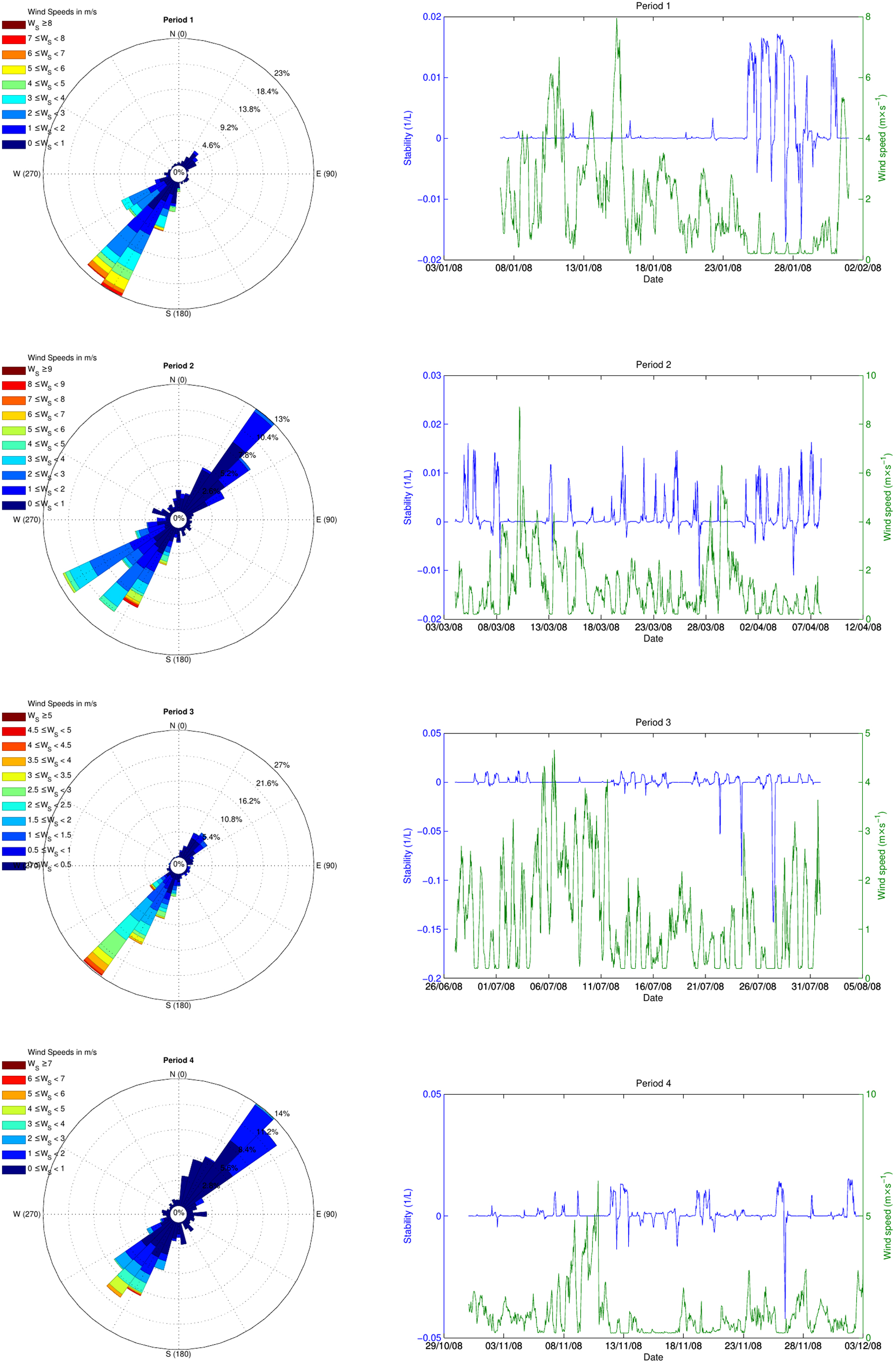
Typical wind field and atmospheric stability in the landscape study corresponding to the four periods. Averaging period is 1 h. Wind rose is plotted using windrose code v1.6 showing the prevailing wind directions (Pereira, 2020) (left), and the mean wind speed and the atmospheric stability expressed by the reciprocal of the Monin-Obukhov length 1/L (right). Air temperature, which is not presented in this study, ranges from −4.8°C to 14°C with an average of 7.8°C for period 1; from −3.1°C to 20.1°C with an average of 7.6°C for period 2; from 6.5°C to 28.9°C with an average of 16.7°C for period 3; and from −2.2°C to 15.5°C with an average of 8.3°C for period 4.

The exposure time of the ALPHA sampler measurements was around 1 month where the suitable range of NH₃ concentrations was 0.03–100 NH₃ μg/m³ (CEH, 2021). ALPHA samplers were stored in a cold room until analysis in the laboratory by INRA chemists trained for this at U.K. Centre for Ecology & Hydrology (CEH), according the protocol adopted by CEH (Tang et al., 2018). Supplementary Table B gives the coefficient of variation calculated for each ALPHA and it shows the good average agreement within triplicates (<9%). The ALPHA samplers were evaluated against the DELTA denuder reference system and shows the good strength between the two ammonia detection systems, R² = 0.991.

Indeed, there was one DELTA sampler permanently installed in the field, which was co-located with 1 of the 28 ALPHA measurement stations. The DELTA denuder sample trains were changed at exactly the same times as the ALPHA samples at this site. Supplementary Figure A provided the comparison of the DELTA sampler with the co-located ALPHA data. The ALPHA time series shown on the comparison plot with the DELTA sampler is the time series of the ALPHA sampler co-located with the DELTA. To check for contamination, a set of field and laboratory blanks was generated for each monthly batch of samplers. Locations of passive ALPHA in the experiment study area are shown in Fig. 3 by “plus.”

Meteorological data and dispersion modelling

The standard meteorological records, offered from the Agroclim agency, were provided by a station located within the experimental domain with an averaging period of 1 h. These include the wind speed, wind direction, temperature, relative humidity, rainfall, and solar radiation. Given that cloud cover measurements were unavailable in the site, an equivalent cloud cover (nnc) was calculated using the solar radiation, R, and the clear sky insolation, R_o, as follows (Cimorelli et al., 2005):

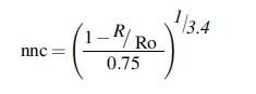
Figure 1 shows the atmospheric stability for each measurement period, as well as the wind rose indicating the measured wind speed and direction statistics during the four periods, which were plotted using windrose code version 1.6 (Pereira, 2020).

To investigate the impact of the spatial variability of NH₃ emissions, the AERMOD was applied to predict monthly average air NH₃ concentrations at a landscape scale, at a 25 × 25 m² grid resolution (Cimorelli et al., 2005). This Gaussian plume model uses the Monin-Obukhov similarity theory rather than the ordinary stability classes (Pasquill and Smith, 1983) which is a more up-to-date representation of state of the atmosphere (Foken, 2006).

The friction velocity (u*) and the mixing height (L) were computed through an iterative process (Cimorelli et al., 2005), as it is done in the present simulations or may be provided in the input file.

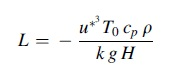
where C_p is the specific heat capacity of air, k is the von Karman constant, g is the acceleration due to gravity, ρ is the density of the air, H is the heat flux, and T₀ is the temperature at the surface. This atmospheric stability indicator is negative (positive) for an unstable (stable) situation, whereas |L| >> 1 indicates neutral situation.

AERMOD simulates dry deposition processes using resistance models; it has seasonal parameterizations for such processes based on land cover types. Dry and wet deposition of NH₃ were included in the simulations in only unidirectional exchange, but due to the absence of the surface characteristics in the entire study area, deposition rates were then not presented in this study. Chemical reactions of NH₃ in the atmosphere were also assumed to be negligible for short-range dispersion.

Emissions were modeled as elevated point sources with an effective diameter of D_S = 20 m, vertical exit velocity V_S = 0 m/s, and exit temperature is T_S = T the ambient temperature. The standard input variables and parameters used to run the model are summarized in Table 2 and in Souhar et al. (2008).

Table 2.

Ammonia Input Variables and Parameters to AERMOD Dispersion Model

Variable	Symbol/value	Unit	Measurement site
Wind speed	u	m/s	Met. station (z = 1.8 m)
Wind direction	—	°	Met. station (z = 1.8 m)
Friction velocity	u∗	m/s	Met. station
Monin_obukhov length	L	M	AERMOD pre-processor
Rainfall rate	P	mm/h	Met. Station
Air temperature	T	°C	Met. station (z = 1.8 m)
Relative humidity	RH	%	Met. station
Roughness length	Z ₀	m	Estimated (0.05–0.2) Wieringa (1992)
Diffusivity in air	D_a	m²/s	2.29 Massman (1998)
Diffusivity for water vapor in air	D_w	m²/s	2.49 Massman (1998)
Leaf cuticular resistance	R_c	s/m	Estimated (600–1,000) Singles et al. (1998)
Henry's law coefficient	—	Pa m³/mol	1.61
Source release height	H _S	m	Estimated (2–2.5)

Statistical performance parameters

Model performance can be evaluated qualitatively by drawing a scatter diagram using predicted (C_p) and observed (C_o) values when observations are available, whereas a quantitative evaluation is most often made through statistical performance parameters. This evaluation will be done with regard to variations of the roughness length z₀ and heights of point sources H_S. Many statistical performance measures are available (Chang and Hanna, 2004). For the current evaluation, five largely used parameters are applied to investigate the performance of the model (Zou et al., 2010; Vogt et al., 2013; Moreira et al., 2014):

Fractional bias: $F B = 2 \times (\bar{C_{o}} - \bar{C_{p}}) ∕ \bar{C_{o}} + \bar{C_{p}}$

Geometric mean bias: $M G = exp (\bar{ln C_{o}} - \bar{ln C_{p}})$

Geometric mean variance: $V G = exp (\bar{{(ln C_{o} - ln C_{p})}^{2}})$

Normalized mean square error: $N M S E = \bar{{(C_{o} - C_{p})}^{2}} ∕ \bar{C_{o}} \times \bar{C_{p}}$

and the fraction of model predictions within a factor of two of observations (FAC2), where overbars denote the mean of each dataset. FB, based on a linear scale, is a dimensionless symmetrical and bounded number; the FB values range from −2.0 to +2.0 (extreme over and under predictions). Like FB, the MG, although based on a logarithmic scale, measures the mean bias and indicates only systematic errors that always lead to the overestimation (MG <1) or underestimation (MG >1) of the measured values.

The NMSE and VG are composite measures that take into account both scatter and bias to the predicted values relative to the observations. A perfect model would have MG = VG = 1, FAC2 = 100%, and FB = NMSE = 0, a condition that is never satisfied in reality. Thus, the performance of an atmospheric dispersion model can be deemed acceptable if |FB| < 0.3, 0.7 < MG <1.3, 1.0 ≤ VG <4.0, FAC2 > 50%, and NMSE <1.5 (Chang and Hanna, 2004).

Results

Figure 1 shows how many hours per NH₃ concentration measurement periods the wind blows from the indicated direction. Throughout this figure, it can be seen that there is a tendency for south-west to north-east winds within the domain. Wind speeds had seasonal trends, in fact, and using the following wind speed classification: wind speeds below 0.5 m/s occurred 23% of period 1; 30% of period 2; 34% of period 3, and 40% of period 4, while wind speeds above 3 m/s occurred 21% of period 1; 10% of period 2; 7% of period 3, and 4% of period 4. During periods 1 and 4, there was a prevailing SW wind direction, the second direction encountered in period 2 and 3 was from the NE.

Air temperature, which is not presented in this study, had also large seasonal trends. The boundary layer structure is described using Monin-Obukhov length and boundary layer height rather than using Pasquill stability categories. Period atmospheric stabilities were estimated as the reciprocal of the Monin-Obukhov length (1/L) (Foken, 2006). Figure 1 shows that a neutral stratification occurred over the entire period 1, except for the last week where obviously stability/unstability took place, while moderate stable and unstable stratifications occurred overall the entire period 2, period 3, and period 4.

The evaluation of emission inventories at a landscape scale should proceed through the quantification of the emissions from farm-scale sources. Thus, emission rates, given in Table 1, are estimated by cumulating individual emissions from livestock housing and manure storage, land spreading of manures, and fertilizer N application. NH₃ emission rates in the current experimental area are predominantly associated with livestock housing, waste storage, and land application of manure, which account for 80% of total NH₃ emissions.

This result is in line with the 2018 annual national emissions inventory where it is shown that these three sources account for 76% of the total NH₃ emissions (Air Breizh, 2019). The total emissions were estimated at 5.92, 8.16, 7.37, and 7.29 NH3 t per period 1, 2, 3, and 4, respectively, leading to a nearly constant daily emission rate of 225 NH₃ kg/day for all periods. NH₃ emission estimates are made according to the French inventory of gaseous emissions (Bioteau et al., 2011) and by using data given in the (Supplementary Table A).

ALPHA samplers fall into two sets: (i) samplers placed roughly NE of source areas upwind the prevailing wind direction and (ii) samplers placed roughly SW of source areas (downwind the second prevailing wind direction). To measure horizontal concentration gradients, samplers were placed at different distances from the source areas at the same height of 2 m. Monthly NH₃ concentration measurements for all periods have a large spatial variability ranging from 2.83 to 105.17 for period 1; 3.57 to 76.08 for period 2; 2.86 to 67.15 for period 3, and 1.77 to 64.27 NH₃ μg/m³ for period 4.

Figure 2 gives a scatter diagram between predicted and observed concentrations at a 2 m height for the four measurement periods with H_S = 2.5 m for all periods, and z₀ = 0.10, 0.20, 0.20, and 0.15 m for periods 1, 2, 3, and 4, respectively. It provides an immediate visualization of the overall AERMOD performance and it shows that the predicted concentrations are in good agreement with the observed ones for periods 2 and 3, while these predicted concentrations are overestimated for periods 1 and 4. However, for all periods, the measured and modeled NH₃ concentrations were highly correlated (R² > 0.96).

FIG. 2.

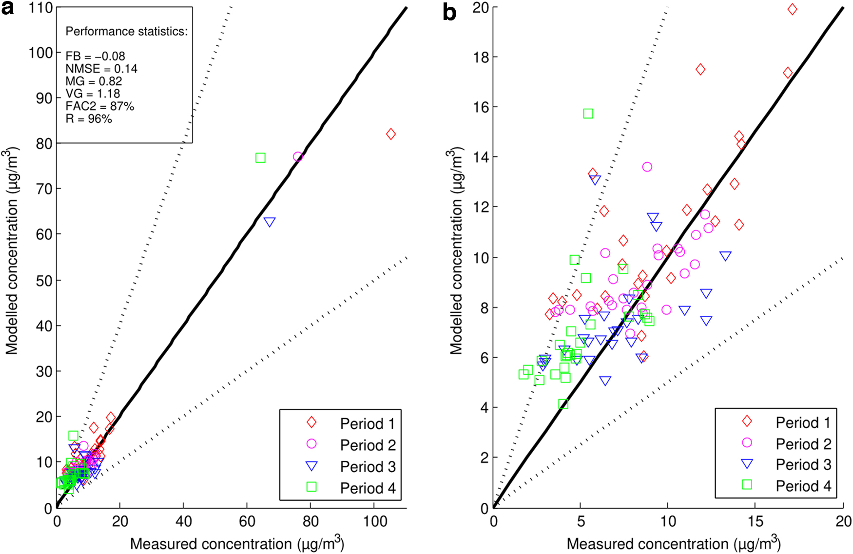
AERMOD modeled NH₃ concentrations versus measured concentrations at height of 2 m for H_S = 2.5 m for all periods, while z₀ = 0.10 m, 0.20 m, 0.20 m, and 0.15 m for periods 1, 2, 3, and 4, respectively. The data points are plotted separately during the four periods (a) and a zoom on the scatter diagram (b). The solid line is the one-to-one between modeled and observed concentrations, whereas the dotted lines correspond to factor of two. The box at the upper left gives the statistics, calculated for the four periods, used to assess the model's performance. NH₃, ammonia.

Figure 3 clearly shows the high spatial variation of NH₃ concentration (μg/m³) at the height of 2 m above the ground in the experiment domain using 25 × 25 m² grid squares and hourly temporal resolutions.

FIG. 3.

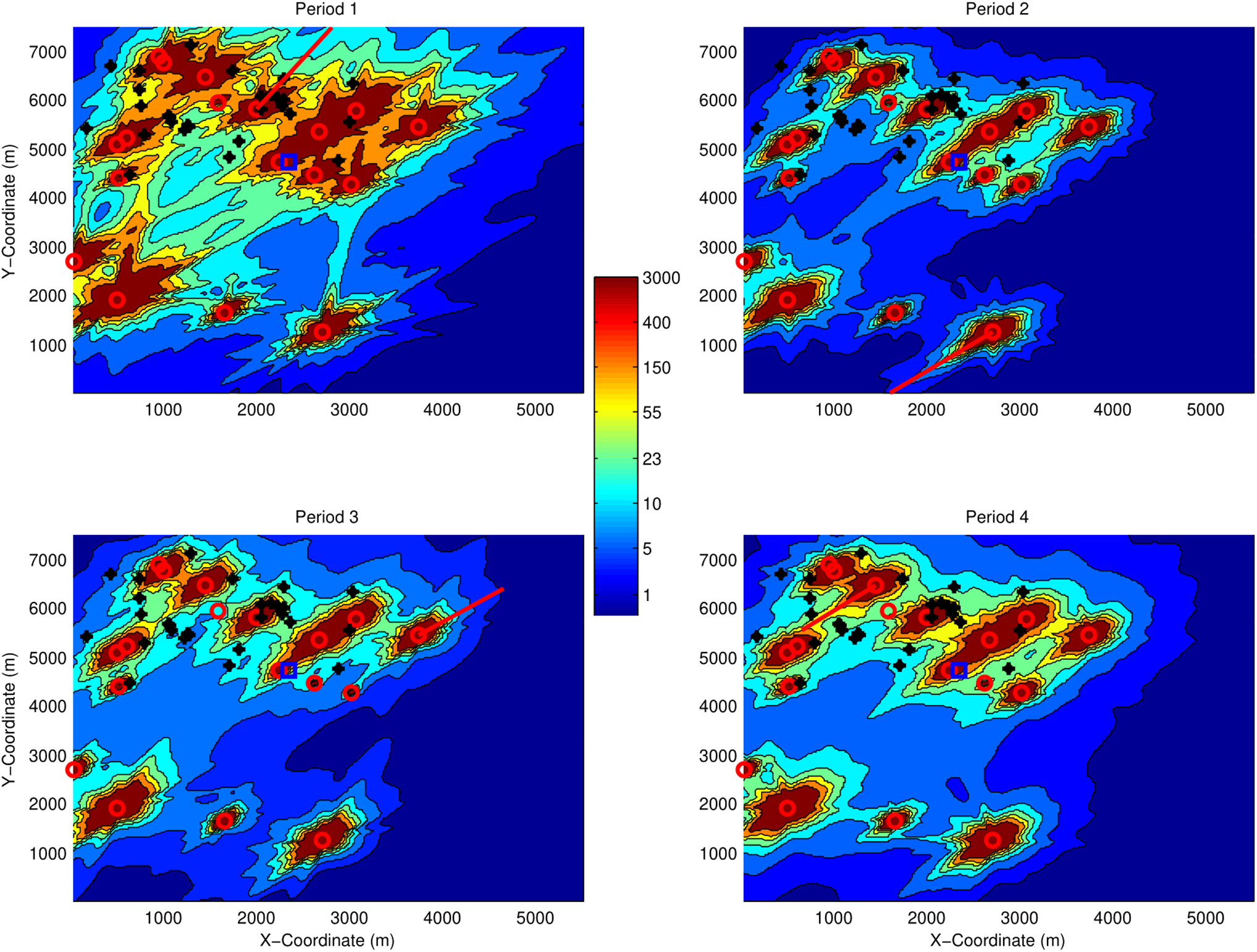
Spatial variation in NH₃ concentration (μg/m³) at height of 2 m during the four periods for the study area, which is considered a flat terrain with H_S = 2.5 m for all periods, and z₀ = 0.10 m, 0.20 m, 0.20 m, and 0.15 m for periods 1, 2, 3, and 4, respectively. Sources and samplers are plotted, respectively, by o and +, while the meteorological station is presented by a blue square. Red lines present the transect concentrations shown in Figs. 4 and 5.

The modeled distribution across the landscape is strongly heterogeneous. The highest concentration levels are marked along the centerline around the livestock building and manure storage facilities (<50 m); for example, concentrations approximately reach 2,900 NH₃ μg/m³ close to the source areas, while around 100 m from the source areas, the concentrations are predicted >100 NH₃ μg/m³. The lowest concentrations are observed in the long way areas from sources. Note that the spread of the pollutant and the shape of the plume vary slightly between periods of the year, that is, they vary according to the meteorological data and depend particularly on the wind speed and the atmospheric stability.

The UNECE has recommended the monthly CLE at 23 NH₃ μg/m³ as a provisional value for croplands to deal with the possibility of high peak emissions during periods of manure application (e.g., in spring) (UNECE, 2007). This critical level is, of course, merely indicative and is subject to change as required since there is no scientific research that supports this value. The monthly provisional CLE exceedance in our domain is estimated from the measured and modeled period average atmospheric NH₃ concentrations.

As a consequence, the areas that exceeded the CLE occur then in the vicinity of the sources (< ∼350 m) and account for 24%, 16%, 15%, and 17% from the total area for periods P1, P2, P3, and P4, respectively. From the Supplementary Table A, it seems that high concentrations occur through the year. In addition, a part from the French national guide to good agricultural practices to limit NH₃ emissions by developing methodologies and technologies to reduce NH₃ emissions, there are little opportunities for recovery in the few future years since there is no direct potential cost implication for farmers.

To illustrate concentrations close to source areas, a separate farm was considered where the influence from other sources of NH₃ is negligible as marked by the red line in Fig. 3 (Panel: period 2). The suitable farm corresponds to Livestock 8 in Table 1, where the emission rate is as follows: for period 1, Q = 19.42 NH₃ kg/day; and for periods 2, 3, and 4, Q = 29.73 NH₃ kg/day. Figure 4 illustrates the AERMOD concentration profiles at 2 m height plotted against the distance in the prevailing wind direction for the four periods. The figure shows the same log-scale behavior of the concentration for all periods; concentration decreased with increasing distance in the prevailing wind direction and the horizontal gradient at 2 m above the ground is generally smooth. Red line presents a simple model to simulate the NH₃ concentration profile provided as the simple decay curve

where x is the distance from the point source of 2.5 m height, emitting Q (NH₃ kg/day) depending on periods. It should be noted that the simple decay curve is obtained from the average of simple models given by Thöni et al. (2004) to simulate the concentration profile of Asman and van Jaarsveld (1990) near and far from the point source. An immediate visualization shows that the simple model tended to have a good performance to simulate the AERMOD concentration profiles in the prevailing wind direction. Furthermore, relative errors by period are as follows; RelErr(P1) = 0.36, RelErr(P2) = 0.17, RelErr(P3) = 0.38, and RelErr(P4) = 0.13. Relative error is defined as the ratio of differences in concentrations obtained by AERMOD and the simple decay curve and those simulated by AERMOD.

FIG. 4.

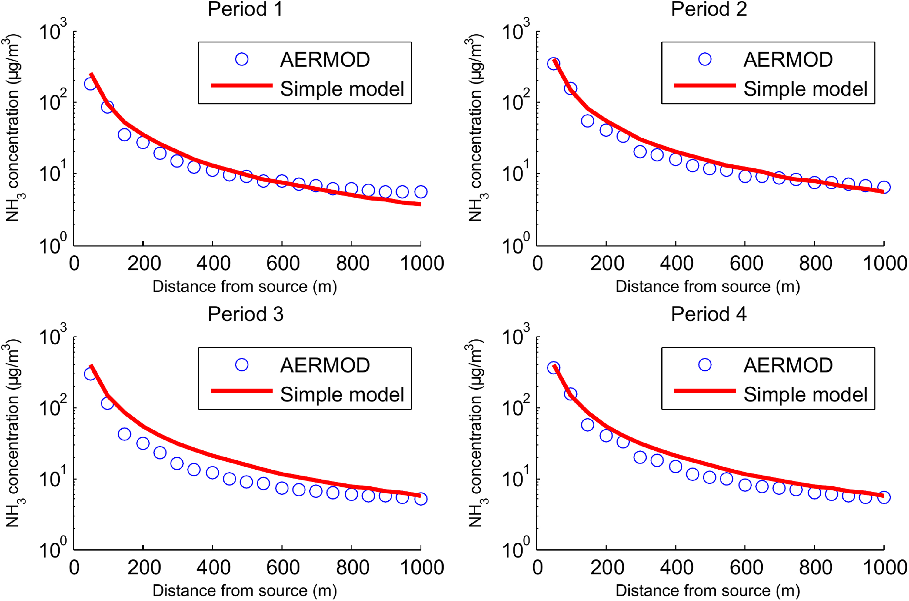
Horizontal crosswind concentration profiles (corresponding to the red line in Fig. 3, Panel: period 2) plotted on a log-scale in the prevailing wind direction distance of the same source of 2.5 m height. Solid red line is the simple model given by C(x) = Q*365*(15.197*x − 1.3922 + 8.38*x − 1.8235)/2 where x is the distance in the prevailing wind direction of the point source emitting Q (NH₃ kg/year).

By specifying the receptor network in the input file for AERMOD (Cimorelli et al., 2005), Fig. 5 shows the modeled vertical profile of NH₃ concentrations, marked by the red lines in Fig. 3, at different distance from 50 to 1,000 m from the source areas for each period. Emission rates Q₁ = 15.42, Q₂ = 29.73, Q₃ = 18.04, and Q₄ = 19.61 NH₃ kg/day for periods 1, 2, 3, and 4 are emitted, respectively, from Livestock 1, 8, 13, and 17 in Table 1.

FIG. 5.

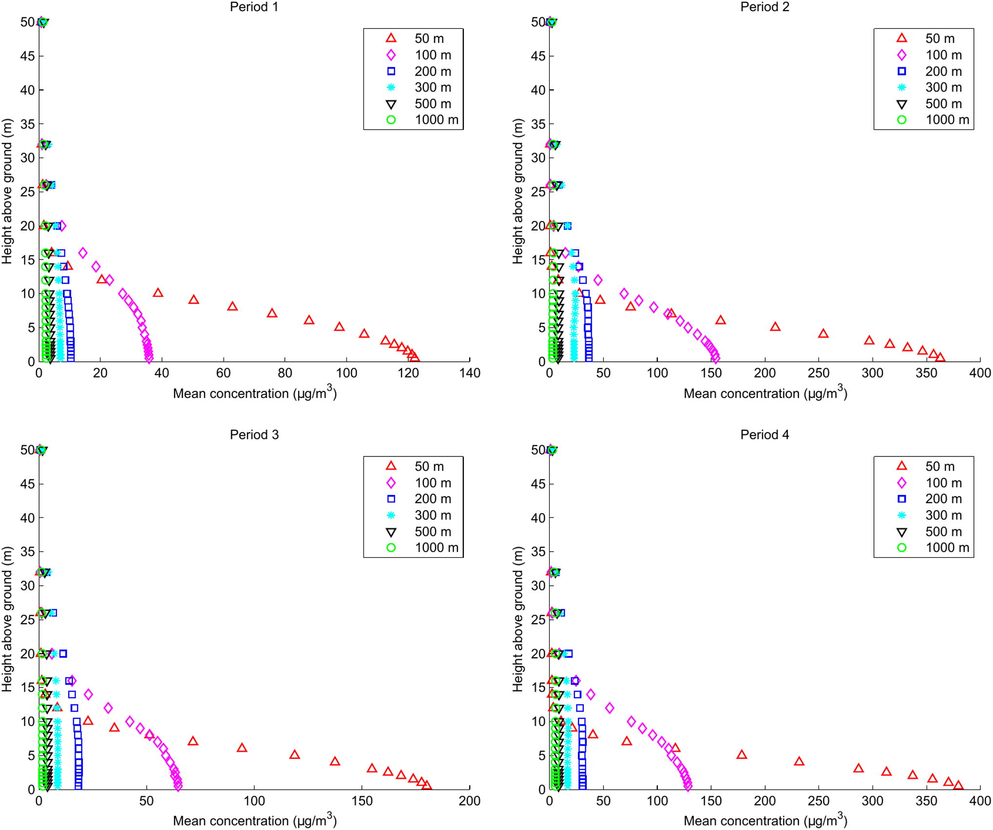
Vertical concentration profiles of NH₃ (corresponding to red lines in Fig. 3) with distance from 50 to 1,000 m in the prevailing wind direction of sources and at different heights from 0.5 to 50 m.

Areas of the higher modeled concentration are observed close to the livestock housing and manure storage facilities, as well as near the ground level, and the peak concentrations are at a height of 0.5 m and the lowest concentrations are predicted far from sources. It should be noted that concentrations above 30 m are small and homogenous in the experiment study area and approximately are unvarying with the height at 1,000 m. In conclusion, Fig. 5 also demonstrates how areas in the prevailing wind direction and near the source placements receive the largest concentrations.

At local scale, concentrations of NH3 are sensitive to multiple parameters such as the source height, land cover type, wind speed, atmospheric stability, and specific surface parameters. As it is already mentioned in the MM section, the source height and the roughness length are very approximate in the simulation part; it is thus judicious to carry out a brief study of sensitivity analysis with respect to variations of these two parameters. Two values of z₀ and H_S for each period were simulated, which leads to 448 predicted values (28 sampler localizations × 2 roughness lengths × 2 building heights × 4 periods), which were used to assess the quantitative evaluation of the model by considering the statistical parameters FB, MG, NMSE, VG, and FAC2.

In fact, of the total simulated values, 87% are within factor of two (FAC2) of the observations, and all statistical parameters values are mostly within the range of acceptable model performance. This result essentially shows that the source height and roughness length are well estimated. However, the parameterized turbulence near the surface may not necessarily be an accurate representation of real atmospheric conditions. Indeed, by analyzing and depicting the encountered results provided in Table 3 according to each period, it shows that the predicted concentrations are overestimated in general by the model for all periods. These overestimations are well marked for period 1 and period 4 (corresponding to cold seasons) where MG is outside the performance range.

Table 3.

Summary of Five Statistical Performance Parameters Calculated for the 28 Observations With Regard to Variations of the Roughness Length z₀ and the Source Height H_S

Statistical parameters	Period 1	Period 2	Period 3	Period 4	Target performance
FB	−0.05	−0.02	−0.03	−0.28	\|FB\| < 0.3
NMSE	0.15	0.14	0.07	0.20	<1.5
MG	0.83	0.91	0.89	0.69	0.7 < MG <1.3
VG	1.15	1.15	1.13	1.28	1.0 ≤ VG <4
FAC2	86%	89%	93%	0.82%	FAC2 > 50%

Discussion

The aim of this work is to validate the AERMOD under different situations for an intensive agricultural landscape as well as to give a spatial variability of atmospheric NH₃, and therefore provide areas with high concentrations. To best model the dispersion of NH₃, the results show that it is important to accurately provide measurement and estimation of NH₃ emissions, which constitute the main challenge with regulation of NH₃ from agriculture (Hellsten et al., 2008). In fact, atmospheric NH₃ emissions cannot easily be directly quantified due, for example, to a bad knowledge of emission from the sources, in both time and space. It is also due to inaccurate estimates of NH₃ emission dynamics at the daily, seasonal, and annual time scale for a diversity of animal species, building types, and effluent management practices (Dragosits et al., 2002; Pinder et al., 2004).

Species, number, and age of the livestock are major determinants of NH₃ emission. NH₃ emissions from housing and storage are highly variable in space and time depending not only on the type and number of animals present in each livestock building but also on the housing duration leading to seasonal/daily emission variability (Anderson et al., 2003; Aneja et al., 2003; Battye et al., 2003). Due to the large uncertainty in emission estimates, the application of atmospheric measurements and inverse modeling is perhaps the most interesting methodology to accurately quantify the emissions of NH₃ (Flesch et al., 2009; Harper et al., 2010; Bell, 2017).

In this study, the emission rates are assumed to be constant per period and the point sources with a single release height. In reality, each point source is composite of individual source areas with multiple release heights ranging from ground level to several meters above the ground. The influence of these simplifications could directly move the vertical and crosswind dispersion of the plume, which hence impacts the spatial distribution of NH₃. Moreover, Bell (2017) has shown that changing source release height from 1 to 0 m caused a 64–76% increase in emissions leading to a considerable reduction in simulated concentrations. Ammonia emissions and their air concentrations are highly temporally variable and the assessment of ammonia is usually made annually. As a consequence, the use of these 1-month periods should necessarily be the important downside of our approach.

The emission plume is originated from the ground level, then the turbulent mixing near the land surface (a function of z₀) is more important, and plume depletion due to deposition could also reduce the atmospheric concentrations. The pattern of the pollutant dispersion is a slowly expanding plume due to the low magnitude of wind speed for all periods as well as because of the high deposition velocity of NH₃; most of the NH₃ is deposited close to the source (Dragosits et al., 2002; Vogt et al., 2013; Kelleghan et al., 2021). As a consequence, the highest monthly concentrations (>23 NH₃ μg/m³) occur then in the vicinity of point sources (< ∼350 m) where areas are arable cropping and grazing, which could have potential impacts on both the health of the farmers and their crops.

The horizontal gradient at 2 m above the ground is generally smooth in the prevailing wind direction from sources. The results are in line with those provided by Loubet et al. (2006) during the “Bretagne 99” experiment.

The AERMOD has a tendency to predict higher concentrations at 2 m height compared to measurements, which is in line with previous intercomparisons of this model (Theobald et al., 2012). In addition, Bajwa et al. (2008) showed that AERMOD underestimated NH₃ dry deposition for grass and short vegetation and therefore overestimates air concentrations. This overestimation may also be explained by the fact that the roughness length and the release height are not well estimated and/or related to the parameterization of the atmospheric stability of the model. Wind speed greatly influences local concentration.

In fact, an increase in the wind speed generates an increase in the turbulent diffusion that has the consequence of decreasing the surface concentration, which may give reason for results obtained during periods 1 and 4. During period 4, low wind speeds (below 0.5 m/s) occur 40% with moderate stable and unstable stratifications, which led to higher concentrations than the measured ones. Under low winds, the advection no longer dominates over diffusion; therefore, it becomes difficult to accurately simulate concentrations using a dispersion model. Although AERMOD includes routines for such situations, it is still difficult to simulate accurately the NH₃ dispersion as also shown by Theobald et al. (2015).

The overestimations, during period 1, may be either due to the roughness length or to the atmospheric stability of the model. By the use of the OPS-st, a plume model for local scale application, the source height and the surface roughness affect strongly the concentration within a few 100 m from the source (Asman et al., 1998). At this short distance, the concentration can decrease up to 60% with a higher point of emission and by higher roughness. The overestimations during these two cold periods are also linked to the use of an annual average emission rate rather than seasonal rate, which is an important limitation of this study.

In the same way, but only quantitatively, statistical indices given in Table 3 show that the performance of the model depends separately on local particularities of each experiment, although the calculated values are mostly within the range of acceptable model performance, that is, small variations in the source height and the roughness length have more influence on air concentrations for periods 1 and 4 than for periods 2 and 3.

Knowing the uncertainty in the source estimates (Dragosits et al., 2002; Pinder et al., 2004), AERMOD is found to be a good model among existing atmospheric models being applied at the landscape scale.

The observed discrepancies between the modeled and measured NH₃ concentrations may be due to cumulating uncertainties involving (Loubet et al., 2006):

(i) as detailed above, uncertainty in NH₃ emissions;

(ii) errors due to uncertainties in the localization of sources and samplers, and the large horizontal concentration gradients near point sources;

(iii) another potential source of these overestimations that should be suspected is linked to the depletion through dry deposition. Asman et al. (1998) and Loubet et al. (2009) have estimated that 20–75% of the NH₃ plume may be depleted within 2 km downwind of the source;

(iv) uncertainties are linked to the transport and the transforming processes in the atmosphere; and

(v) uncertainties are involved by the dry deposition process because of the absence of data to calculate the roughness length. A short-range dry deposition of NH₃ is estimated to be the dominant deposition mechanism and wet deposition may be ignored (Loubet et al., 2009).

Although the results are acceptable for this study, concentration predictions can be improved by introducing the following four important processes in the AERMOD model: (i) the plant canopies can act both as a sink for or a source of atmospheric NH₃, not only as a net sink that is a simplified hypothesis in the AERMOD; (ii) the interactions between different pollutants may be taken into account; (iii) even if the model can now introduce different surface roughness coefficients, the way that it takes this into account is very limited and should be improved; and (iv) the boundary conditions need to be taken into account.

Conclusion

The AERMOD model was applied to simulate the atmospheric dispersion of NH₃ during four periods and under different stability conditions of the year 2008 at 25 × 25 m² grid resolution over a rural landscape containing intensive agricultural farms. Period average NH₃ concentrations at 2 m height above ground level were simulated and compared to measured ones. The analysis showed that modeled and measured values were in good agreement for two periods with moderate wind speeds and atmospheric stability. In addition, although the calculated statistical indices were mostly within the range of acceptable model performance, AERMOD estimates high NH₃ concentrations for some particular situations (period 1 and period 4). Our study has shown that concentrations are high near and downwind from the sources and have strong vertical and horizontal gradients.

Footnotes

Acknowledgments

The first author wishes to thank P. Cellier, J.L. Drouet, and B. Loubet (EcoSys INRAE-AgroParisTech, France) for their helpful discussions, as well as M. Mifdal, Professor of English at Chouaib Doukkali university, for editorial advice about English.

Authors’ Contributions

O.S.: conceptualization, methodology, software, validation, writing-original draft, review, and editing.

Y.F.: reviewing.

C.F.: conceptualization, methodology, and editing.

Author Disclosure Statement

No competing financial interests exist.

Funding Information

No funding was received for this article.

Supplementary Material

References

ADEME. (2019a). Guide des bonnes pratiques agricoles pour l'amélioration de la qualité de l'air, Rapport, Juin-2019, 116p.

ADEME. (2019b). Guide des bonnes pratiques agricoles pour l'amélioration de la qualité de l'air, Synthèse de l'étude, www.ademe.fr (accès 20 octobre 2021), mai 2019, 7 p.

Air Breizh. (2019). Rapport annuel, Rapport interne, 2019, 87p. (accès 20 octobre 2021) https://www.airbreizh.asso.fr/voy_content/uploads/2020/06/rapport-annuel-2019-v6.pdf

Anderson

, Strader

, and Davidson

(2003). Airborne reduced nitrogen: Ammonia emissions from agriculture and other sources. Environ. Int. 29, 277.

Aneja

V.P.

, Nelson

D.R.

, Roelle

P.A.

, Walker

J.T.

, and Battye

(2003). Agricultural ammonia emissions and ammonium concentrations associated with aerosols and precipitation in the southeast United States. J. Geophys. Res. Atmos. 108, 1.

Asman

W.A.H.

, Sutton

M.A.

, and Schjoerring

J.K.

(1998). Ammonia: Emission, atmospheric transport and deposition. New Phytol. 139, 27.

Asman

W.A.H.

, and van Jaarsveld

H.A.

(1990). A variable-Resolution Statistical Transport Model Applied for Ammonia and Ammonium. Bilthoven, the Netherlands: National Institute of Public Health and Environmental Protection (RIVM).

Bajwa

, Arya

S.P.

, and Aneja

V.P.

(2008). Modeling studies of ammonia dispersion and dry deposition at some hog farms in North Carolina. J Air Waste Manag. Assoc. 58, 1198.

Battye

, Aneja

V.P.

, and Roelle

P.A.

(2003). Evaluation and improvement of ammonia emissions inventories. Atmos. Environ. 37, 3873.

10.

Bell

(2017). Emission, Dispersion and Deposition of Ammonia from the Plot to the Landscape Scale. Doctoral thesis, Université Européenne de Bretagne, Rennes, France.

11.

Beusen

A.H.W.

, Bouwman

A.F.

, Heuberger

P.S.C.

, Van Drecht

, and Van Der Hoek

K.W.

(2008). Bottom-up uncertainty estimates of global ammonia emissions from global agricultural production systems. Atmos. Environ. 42, 6067.

12.

Bioteau

, Gac

, and Béline

(2011). Evaluation et Spatialisation des Emissions GAzeuses liées à la gestion des déjections d'élevage (ESEGA): de l'inventaire au test de technologies de réduction des émissions gazeuses. Ingénieries—EAT, IRSTEA édition, 2007, 19.

13.

Carruthers

D.J.

, Holroyd

R.J.

, Hunt

J.C.R.

, Weng

W.S.

, Robins

A.G.

, Apsley

D.D.

, Thompson

D.J.

, and Smith

F.B.

(1994). Uk-Adms - a new approach to modeling dispersion in the earths atmospheric boundary-layer. J. Wind Eng. Ind. Aerod. 52, 139.

14.

Centre for Ecology & Hydrology (CEH). (2021). Air sampler systems for environmental monitoring. https://www.ceh.ac.uk/services/air-samplers (accès 20 octobre 2021).

15.

Chang

J.C.

, and Hanna

S.R.

(2004). Air quality model performance evaluation. J. Meteorol. Atmos. Phys. 87, 167.

16.

Cimorelli

A.J.

, Perry

S.G.

, Venkatram

, Weil

J.C.

, Paine

R.J.

, Wilson

R.B.

, Lee

R.F.

, Peters

W.D.

, and Brode

R.W.

(2005). AERMOD: A dispersion model for industrial source applications. Part I: General model formulation and boundary layer characterization. J. Appl. Meteorol., 44, 682.

17.

Dragosits

, Theobald

M.R.

, Place

C.J.

, Lord

, Webb

, Hill

, ApSimon

H.M.

, and Sutton

M.A.

(2002). Ammonia emission, deposition and impact assessment at the field scale: A case study of sub-grid spatial variability. Environ. Pollut. 117, 147.

18.

Flesch

T.K.

, Harper

L.A.

, Powell

J.A.

, and Wilson

J.D.

(2009). Inverse-dispersion calculation of ammonia emissions from wisconsin dairy farms. Trans. ASABE, 52, 253.

19.

Foken

(2006). 50 Years of the Monin-Obukhov similarity theory. Bound. Layer Meteorol. 119, 431.

20.

Frati

, Santoni

, Nicolardi

, Gaggi

, Brunialti

, Guttova

, Gaudino

, Pati

, Pirintsos

S.A.

, and Loppi

(2007). Lichen biomonitoring of ammonia emission and nitrogen deposition around a pig stockfarm. Environ. Pollut. 146, 311.

21.

Harper

L.A.

, Flesch

T.K.

, and Wilson

J.D.

(2010). Ammonia emissions from broiler production in the San Joaquin Valley. Poult. Sci. 89, 1802.

22.

Hellsten

, Dragosits

, Place

C.J.

, Vieno

, Dore

A.J.

, Misselbrook

T.H.

, Tang

Y.S.

, and Sutton

M.A.

(2008). Modelling the spatial distribution of ammonia emissions in the UK. Environ. Pollut. 154, 370.

23.

Huang

, and Guo

(2019). Dispersion modeling of odour, gases, and respirable dust using AERMOD for poultry and dairy barns in the Canadian Prairies. Sci. Tot. Environ. 690, 620.

24.

Kelleghan

D.B.

, Hayes

E.T.

, Everard

, and Curran

T.P.

(2021). Predicting atmospheric ammonia dispersion and potential ecological effects using monitored emission rates from an intensive laying hen facility in Ireland. Atmos. Environ. 247, 118214.

25.

Loubet

, Asman

W.A.H.

, Theobald

M.R.

, Hertel

, Tang

Y.S.

, Robin

, Hassouna

, Dammgen

, Genermont

, Cellier

, and Sutton

M.A.

(2009). Ammonia deposition near hot spots: Processes, models and monitoring methods. In M.A. Sutton, S. Reis, and S.M.H. Baker, Eds., Atmospheric Ammonia Detecting Emission Changes and Environmental Impacts. Dordrecht: Springer, p. 205.

26.

Loubet

, Cellier

, Milford

, and Sutton

M.A.

(2006). A coupled dispersion and exchange model for short-range dry deposition of atmospheric ammonia. Q. J. R. Meteorol. Soc. 132, 1733.

27.

Massman

W.J.

(1998). A review of the molecular diffusivities of H₂O, CO₂, CH₄, CO, O₃, SO₂, NH₃, N₂O, NO and NO₂ in air, oxygen and N₂ near STP. Atmos. Environ. 32, 1111.

28.

Moreira

D.M.

, Moraes

, Goulart

A.G.

, and Albuquerque

(2014). A contribution to solve the atmospheric diffusion equation with eddy diffusivity depending on source distance. Atmos. Environ. 83, 254.

29.

Pasquill

, and Smith

F.B.

(1983). Atmospheric Diffusion. , 3rd ed, New York: Wiley.

30.

Pereira, D. (2020). Wind Rose. MATLAB Central File Exchange. Retrieved May 8, 2020. https://www.mathworks.com/matlabcentral/fileexchange/47248-wind-rose (Accessed March 12, 2021).

31.

Pinder

R.W.

, Pekney

N.J.

, Davidson

C.I.

, and Adams

P.J.

(2004). A process based model of ammonia emissions from dairy cows: Improved temporal and spatial resolution. Atmos. Environ. 38, 1357.

32.

Singles

R.J.

, Sutton

M.A.

, and Weston

K.J.

(1998). A multi-layer model to describe the atmospheric transport and deposition of ammonia in Great Britain. Atmos. Environ. 32, 393.

33.

Souhar

, Cellier

, and Loubet

(2008). Description and comparison of some transport and deposition atmospheric models: LADD, OML, OPS and AERMOD. Technical Report, INRAE AgroParisTech EGC, Grignon, p. 10.

34.

Sutton

M.A.

, Tang

Y.S.

, Miners

, and Fowler

(2001). A new diffusion denuder system for long-term regional monitoring of atmospheric ammonia and ammonium. Water Air Soil Pollut. Focus, 1, 145.

35.

Tang

, Cape

, and Sutton

(2001). Development and types of passive samplers for monitoring atmospheric NO2 and NH3 concentrations. ScientificWorldJournal. 1, 513.

36.

Tang

Y.S.

, Braban

C.F.

, Dragosits

, Dore

A.J.

, Simmons

, van Dijk

, Poskitt

, Dos Santos Pereira

, Keenan

P.O.

, Conolly

, Vincent

, Smith

R.I.

, Heal

M.R.

, and Sutton

M.A.

(2018). Drivers for spatial, temporal and long-term trends in atmospheric ammonia and ammonium in the UK. Atmos. Chem. Phys. 18, 705.

37.

Theobald

M.R.

, Løfstrøm

, Walker

, Andersen

H.V.

, Pedersen

, Vallejo

, and Sutton

M.A.

(2012). An intercomparison of models used to simulate the short-range atmospheric dispersion of agricultural ammonia emissions. Environ. Modell. Softw. 37, 90.

38.

Theobald

M.R.

, Sanz-Cobena

, Vallejo

, and Sutton

M.A.

(2015). Suitability and uncertainty of two models for the simulation of ammonia dispersion from a pig farm located in an area with frequent calm conditions. Atmos. Environ. 102, 167.

39.

Thöni

, Brang

, Braun

, Seitler

, and Rihm

(2004). Ammonia monitoring in Switzerland with passive samplers: patterns, determinants and comparison with modelled concentrations. Environ. Monit. Assess. 98, 93.

40.

UNECE. (2007). Review of the 1999 Gothenburg Protocol: Report on the Workshop on Atmospheric Ammonia: Detecting Emission Changes and Environmental Impacts. 39th Session, April 18–20, 2007, Geneva, Switzerland.

41.

Van Jaarsveld

J.A

. (2004). The Operational Priority Substances Model; Description and Validation of OPS-Pro 4.1. RIVM Report 500045001.

42.

Vogt

, Dragosits

, Braban

C.F.

, Theobald

M.R.

, Dore

A.J.

, van Dijk

, Tang

Y.S.

, McDonald

, Murray

, Rees

R.M.

, and Sutton

M.A.

(2013). Heterogeneity of atmospheric ammonia at the landscape scale and consequences for environmental impact assessment. Environ. Pollut. 179, 120.

43.

Wang

, Uno

, Osada

, Itahashi

, Yumimoto

, Chen

, Yang

, and Wang

(2020). Spatio-temporal variations of atmospheric NH₃ over East Asia by comparison of chemical transport model results, satellite retrievals and surface observations. Atmosphere, 11, 900.

44.

Wieringa

(1992). Updating the Davenport roughness classification. J. Wind Eng. Ind. Aerodyn. 41, 357.

45.

Zou

, Zhan

F.B.

, Wilson

J.G.

, and Zeng

(2010). Performance of AERMOD at different time scales. Simul. Modell. Pract. Theory, 18, 612.

Supplementary Material

Please find the following supplemental material available below.

For Open Access articles published under a Creative Commons License, all supplemental material carries the same license as the article it is associated with.

For non-Open Access articles published, all supplemental material carries a non-exclusive license, and permission requests for re-use of supplemental material or any part of supplemental material shall be sent directly to the copyright owner as specified in the copyright notice associated with the article.

0.00 MB

0.02 MB

0.28 MB