Differential Ambient Air Pollution Exposure in a Chronic Obstructive Pulmonary Disease Cohort: The Role of Area-Level Socioeconomic Factors

Abstract

Background: Disparities in environmental exposures have been investigated in a multitude of epidemiologic studies. Many of these studies have demonstrated that minorities and poorer individuals were disproportionately exposed to elevated levels of air pollution and other environmental hazards. To date, differential air pollution exposures have not been assessed in a cohort of individuals with compromised respiratory health. We evaluated the distribution of air pollution exposures in such a cohort by area-level socioeconomic factors. Methods: Data from the National Emphysema Treatment Trial (NETT) (1998–2003), which included 1218 subjects ages 39–84, were linked with air pollution data from the U.S. Environmental Protection Agency Air Quality Systems database. The air pollution data included daily values of fine particulate matter (PM_2.5) and ozone. ZIP code specific exposures were spatially interpolated with the use of log-normal kriged models. This methodology was employed in order to assign exposures in areas with few nearby air pollution monitors. We investigated whether there was evidence of differential air pollution exposure by area-level measures of socioeconomic status (SES). Results: NETT participants experienced varying levels of exposure to ozone and PM_2.5 and increasing cumulative pollutant exposures were associated with decreasing values of area-level SES such as median income, material deprivation, and percent unemployment. Conclusion: There was evidence of increasing air pollution exposure with decreasing area-level measures of SES. This finding adds to the literature on environmental justice and indicates that SES-related inequalities in air pollution exposure could lead to increased adverse health outcomes, particularly among individuals with existing respiratory disease.

Introduction

Social inequalities in air pollution exposures have been investigated in several epidemiologic studies. One of the earliest of these investigations was performed by Freeman et al. in Distribution of Environmental Quality and demonstrated that poorer individuals and minorities residing in Kansas City, St. Louis, and Washington, DC were more likely to have higher exposures to sulfates and total suspended particulates compared to wealthier individuals and Caucasians.¹ Much of the succeeding literature has focused on the unequal burden in environmental hazards experienced by disadvantaged minorities. These studies have suggested that among such groups, there is a higher likelihood of residing close to point sources of pollution, such as industrial plants and waste sites.^2,3 In addition to race, socioeconomic status (SES) is an important social determinant in environmental justice. Brochu et al. studied the association between particulate matter (PM) and area-level SES in the northeastern United States. They reported that individuals with lower SES tended to be exposed to higher levels of PM when compared to higher SES individuals.⁴ A recent nationwide study, published by Miranda et al., reported similar findings.⁵

Despite the expansive nature of the published literature, there is no clear methodological consensus with respect to assessing differential air pollution exposures by socio-demographic characteristics. Several challenges in comparing research findings on systematic racial or socioeconomic disparities in air pollution exposure include the use of different geographical units of analyses (e.g., regional, census tract, and ZIP code level), different analytic methodologies, difficulties in disentangling race and SES, and different measures of exposure.^6,7,8 To date, much of the extant literature on environmental justice has been based on group level variables in the general population.⁷ Less is known on how area-level SES predictors relate to ambient air pollution exposures in an already vulnerable subgroup. This is particularly important in studies that consider the effects of air pollution on respiratory health outcomes since ambient air pollution concentrations and pre-existing health conditions may be modified by area-level SES characteristics.

This article aimed to characterize and quantify the burden of ambient air pollution exposures experienced by a vulnerable subgroup of subjects with chronic obstructive pulmonary disease (COPD). We used both U.S. Environmental Protection Agency (EPA) Air Quality Systems (AQS) pollution data and results from the National Emphysema Treatment Trial (NETT) to detect differences in ambient air pollution exposure with area-level SES factors. Identifying whether there exists evidence of differential exposure in air pollution concentrations based area-level SES factors would contribute to a greater understanding of the potential health risk faced in an already susceptible population.

Methods

Study population

The NETT was a multicenter, randomized controlled trial with the objective of assessing whether lung volume reduction surgery (LVRS) in conjunction with medical therapy was a better long-term treatment for subjects with severe emphysema when compared to medical therapy alone.^9,10 The major outcomes of interest in the study were post-treatment mortality and maximal exercise capacity. Additional outcomes of interest included lung function, as determined by spirometry, distance walked in six minutes and quality of life. During the period 1998–2002, a total of 1,218 participants were enrolled in the study, of which 608 were randomized to LVRS and medical management; 610 were randomized to traditional medical therapy alone, such as steroids and bronchodilators.¹¹

Radiologists characterized emphysema distribution and magnitude in the lungs with chest computed tomography (CT) scans and a visual scoring scale. The aim of the LVRS was to remove 25% to 35% of the lung, with a particular focus on the most affected areas.⁹ Medical histories of all participants were collected at 6, 12, 24, 36, 48, and 60 months after baseline. Participants were followed for an average of 29.2 months.^9,11

Air pollution data

We obtained pollution data from the U.S. EPA AQS database.¹² We restricted these data to average daily ozone levels (1997–2003), and average daily PM_2.5 values (1999–2003). Because exact addresses were not available for NETT participants, we used ZIP codes to define participant place of residence. Participants were assigned residence at the centroid of their ZIP code, as determined by the 2000 census. Values from monitors within specific ZIP codes were used to interpolate pollutant concentrations at the centroid of the ZIP code, and were then merged with the NETT data. Only resident ZIP codes corresponding with kriged ZIP code specific pollution levels, were considered for the analysis, per Liao et al.¹³ Air pollution data were estimated using log-normal kriging, a technique that allows for the estimation of pollutant values in areas that may not be monitored, in which data from nearby monitoring stations are weighted based on distance and number of monitored locations. Participants with the same ZIP code were assumed to share the same level of exposure. In these analyses, daily pollutant concentrations were averaged as a cumulative measure over the duration of the study.

Geographical units of analysis

Aggregate SES data were obtained from the 2000 U.S. Census Summary File 3 (SF3).¹⁴ Variables were obtained at the ZIP code tabulation area (ZCTA) level. Although ZCTA codes are similar to ZIP codes in that they both share the same designation, ZIP codes were developed as a means to expedite postal delivery, whereas ZCTA codes were developed based on characteristics of Census blocks. The ZCTA code is determined by the U.S. Census by calculating the total number of addresses contained within the Census block boundaries. The Census Bureau then assigns the most frequently occurring ZIP code to the Census block tabulation area. In the case where no ZIP code data are available, values from a contiguous block are employed to assign the ZCTA code. Only one ZIP code is assigned to each Census block tabulation area regardless of its size.^15,16

Socio-demographic variables

Measures of area-level socioeconomic deprivation (SED) have been common and effective ways to examine the effect of socioeconomic disparities on health. Indices such as the Carstairs score and the Townsend SED index have been utilized to capture and summarize multiple aspects of SES.^17,18 In our study, we measured area-level SES with the use of the Townsend SED Index, which more readily allowed for the inclusion of Census data. This index was constructed with the following variables: percent of unemployed individuals aged 16 and older, percent renters, percent overcrowding (defined as more than one occupant per room), and percent of individuals that do not own a car. Values of all variables were obtained at the ZCTA level. Percent unemployed and percent overcrowding were log-transformed before being standardized. Percent renters and percent without a car were also standardized before being included in the overall score. Standardization was performed by subtracting the mean value from the variable of interest and dividing it by its standard deviation. These individual z-scores were then summed to yield the overall SED index value. The SED index value was then stratified and ranked by deciles. Additional ZCTA-level variables considered in the analyses included total population, median income, mean earnings, percent urban residents, and percent of individuals living below 200% of the federal poverty level (FPL).

Statistical analysis

Air pollution, Census, and NETT data were merged based on participant ZIP code. Bivariate analyses were performed to assess how ZIP code level variables correlated with cumulative ozone and PM_2.5. ZIP code level variables that were significantly correlated (r>0.3, p-value<0.05) with pollutant concentrations were included in the linear models. Area-level SES variables that were highly correlated with the SED index were not included in the hierarchical models in order to minimize problems associated with multicollinearity. To model cumulative pollutant exposure, models were initially constructed with ZCTA-level SES factors alone, and then with interactions of ZCTA-level SES characteristics. We compared nested linear regression models using a likelihood ratio test or the likelihood-based Akaike's information criterion (AIC).¹⁹ The final linear models included the following covariates: region of residence, SED index deciles, total number of people residing in the ZIP code, median income, and percent of people living below the poverty level in the ZIP code.

The PROC REG procedure was used for the linear regression models. All analyses were performed with SAS 9.2 (SAS Institute Inc, Cary, NC).

Ethics

Approval for this study was received from the Institutional Review Board at The Ohio State University. Because this was a secondary data analysis, no patient contact or consent was required.

Results

Of the original 1,218 participants, there were 1,204 subjects for whom there was complete ozone and PM_2.5 data and whose ZIP codes were also designated in the U.S. Census SF3 database. There were a total of 1,128 unique ZIP codes.

Results of our analyses show evidence of an association between SES measures and air pollution. Specifically, individuals residing in ZIP codes that were in the lowest percentile of the SED index had increased PM_2.5 exposures compared to those residing in the highest percentiles (Figure 1). Although there was more variability seen with cumulative ozone levels, it is still indicative of the trend line of increased exposure among those with a higher SED index (Figure 2). In the bivariate analyses, cumulative ozone was significantly correlated with median income (r=−0.22, p<0.01) and percent below 200% FPL (r=0.11, p<0.01). It was not however correlated with SED index (r=0.04, p=0.14) but it was significantly correlated with the ranked SED index (r=−0.07, p<0.05). Cumulative PM_2.5 was significantly correlated with SED index (r=0.12, p<0.01), ranked SED index (r=−0.11, p<0.01), median income (r=0.11, p<0.01), and percent below 200% FPL (r=−0.1, p<0.01) (Table 1).

FIG. 1.

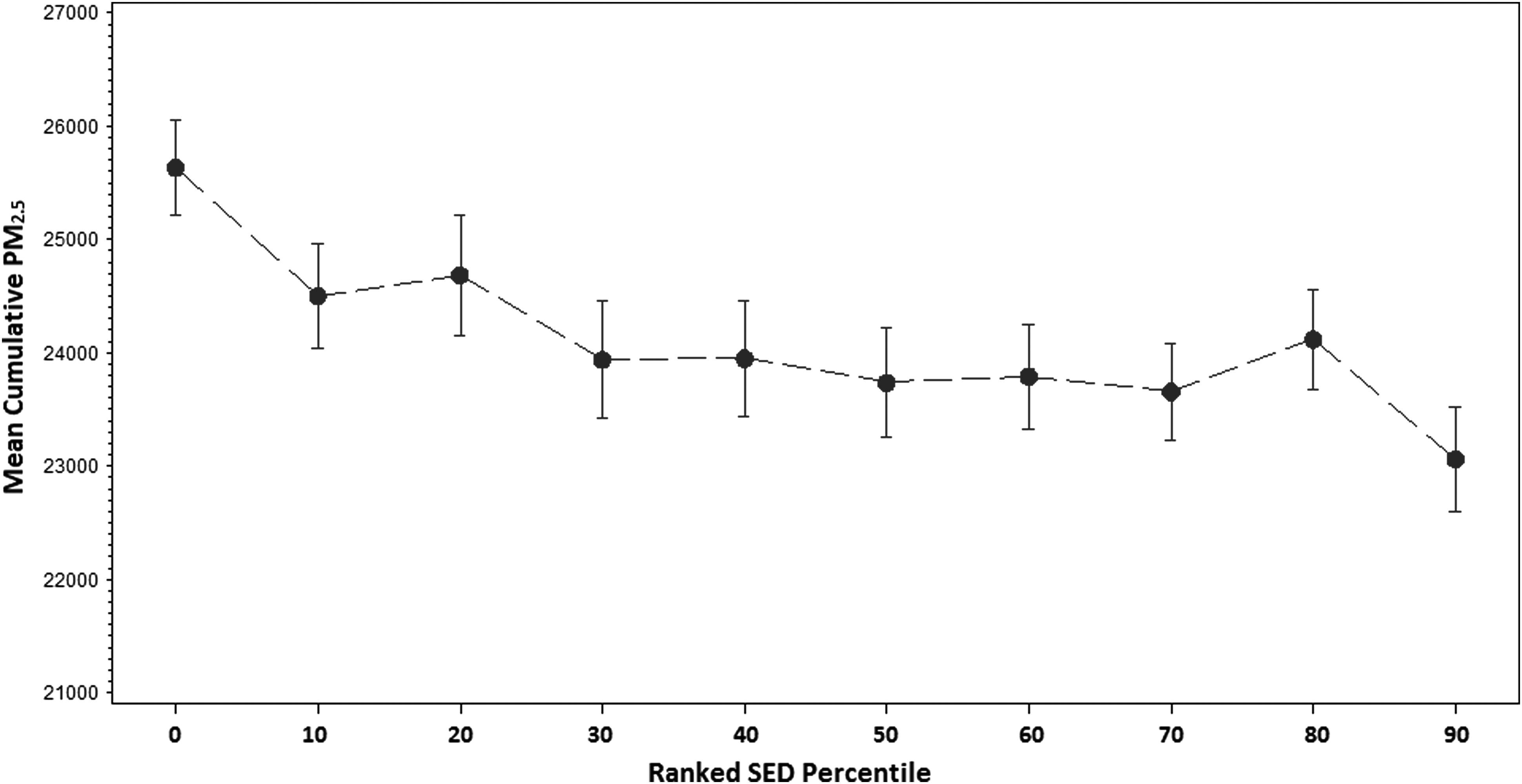
Mean cumulative PM_2.5 by ranked SED index percentile. Mean cumulative PM_2.5 were calculated and plotted against each ranked SED percentile. Error bars represent±1 standard error of the mean. PM_2.5: particulate matter; SED: socioeconomic deprivation.

FIG. 2.

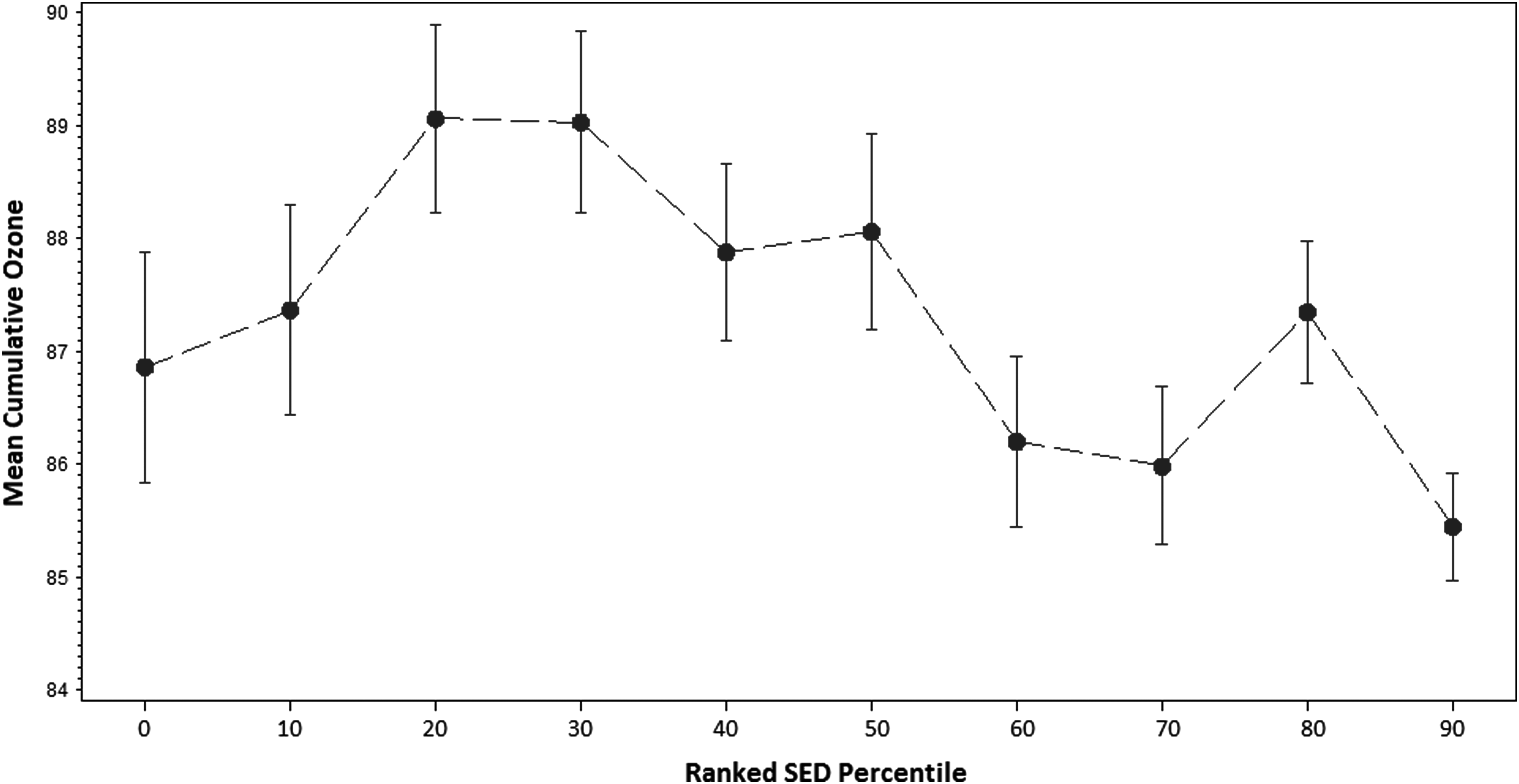
Mean cumulative ozone by SED index percentile. Mean cumulative ozone concentrations were calculated and plotted against each ranked SED percentile. Error bars represent±1 standard error of the mean. SED: socioeconomic deprivation.

Table 1.

Bivariate Spearman Correlations between Individual and ZIP Code-Level Covariates

Variable Name	SED	No Car	Unemployed (log)	Renter	Crowding (log)	Median Income	Percent <200% FPL	Cumulative Ozone	Cumulative PM_2.5	Percent Urban
SED	1	0.56^**	0.52^**	0.32^**	0.45^**	0.13^**	−0.04	0.04	0.12^**	0.30^**
No Car	0.56^**	1	−0.22^**	−0.36^**	0.62^**	0.59^**	−0.21^**	−0.14^**	0.09^**	0.45^**
Unemployed (log)	0.52^**	−0.22^**	1	0.47^**	−0.29^**	−0.45^**	0.26^**	0.21^**	0.05	−0.14^**
Renter	0.32^**	−0.36^**	0.47^**	1	−0.51^**	−0.71^**	0.13^**	0.13^**	−0.02	−0.06
Crowding (log)	0.45^**	0.62^**	−0.29^**	−0.51^**	1	0.8^**	−0.15^**	−0.13^**	0.1^**	0.28^**
Med Income	0.13^**	0.59^**	−0.45^**	−0.71^**	0.8^**	1	−0.11^**	−0.22^**	0.11^**	0.21^**
% Poverty	−0.04	−0.21^**	0.26^**	0.13^**	−0.15^**	−0.11^**	1	0.11^**	−0.1^**	−0.54^**
Cumulative Ozone	0.04	−0.14^**	0.21^**	0.13^**	−0.13^**	−0.22^**	0.11^**	1	0.21^**	−0.07^**
Cumulative PM_2.5	0.12^**	0.09^**	0.05	−0.02	0.1^**	0.11^**	−0.1^**	0.21^**	1	0.11^**
Percent Urban	0.30^**	0.45^**	−0.14^**	−0.06	0.28^**	0.21^**	−0.54^**	−0.07^**	0.11^**	1

SED: socioeconomic deprivation index; FPL: federal poverty level; PM_2.5: particulate matter.

p-value<0.05.

In the cumulative pollutant regression models adjusted for region of residence, SED index deciles, total number of people residing in the ZIP code, median income, and percent of people living below the poverty level in the ZIP code, ranked SED index was significantly associated with cumulative PM_2.5 (Table 2). Increasing SED index decile was associated with a decrease of 155.09 μg/m³ (standard error [SE]=58.11, p<0.01) in cumulative PM_2.5. Individual level factors such as sex and region of residence were all significantly associated with increased cumulative PM_2.5 exposure. Interestingly, median income was significantly associated with increased cumulative PM_2.5 exposure, although the effect was relatively small (β=0.03, SE=0.01, p<0.01). Individual level age and education were not considered as covariates in the cumulative PM_2.5 model as the model focused solely on ZIP-code-level variables.

Table 2.

Regression of Cumulative PM_2.5 Exposure (μg/m³) with ZIP Code-Level SES Variables

Variables	Estimate	SE	p-value
Intercept	19509	679.34	<0.01
Region
Midwest	2715.66	453.13	<0.01
Northeast	3392.08	432.33	<0.01
South	3420.76	443.35	<0.01
West (Referent)	-	-	<0.01
Median Income	0.030	0.01	<0.01
Ranked SED Index	−155.09	58.11	<0.01
Total Population	0.128	0.022	<0.01

PM_2.5: particulate matter; SES: socioeconomic status; SE: standard error; SED: socioeconomic deprivation index.

For the cumulative ozone model, there was a significant negative effect of the ranked SED index (β=−0.32, p=0.02); however this occurred in the presence of a significant interaction between the ranked SED index and total population (Table 3). The only significant covariates in the model were median income, region of residence, and percent living below 200% FPL. Large effect estimates were seen for region of residence in both pollutant models.

Table 3.

Regression of Cumulative Ozone Exposure (Ppm) With ZIP Code-Level SES Variables

Variables	Estimate	SE	p-value
Intercept	93.9	1.26	<0.01
Region
Midwest	−3.29	0.69	<0.01
Northeast	−3.59	0.68	<0.01
South	4.93	0.71	<0.01
West (Referent)	-	-	-
Median Income	−0.0001	0	<0.01
Ranked SED Index	−0.32	0.14	0.02
Total Population	−0.0001	0	0.02
Ranked SED Index^Total Population*	0.000	0.00	0.02
Percent Below Poverty Level	0.069	0.03	0.05

SES: socioeconomic status; SE: standard error; SED: socioeconomic deprivation index.

Discussion

Our findings suggest there is a significant differential exposure to ambient ozone and PM_2.5 exposures among persons with lower area-level measures of SES. As a measure of area-level SES, a higher SED index was clearly and strongly associated with increasing levels of ambient ozone and PM_2.5. Utilizing pollution data from over 1,000 ZIP codes, the NETT study allowed us to assess differential ambient exposures on a national scale (Figure 3). Unlike many previous studies that examined air pollution disparities in the United States, our study is one of the few to consider the effects of Census-based area-level measures of SES on differential pollutant exposures. To date, it is also the only study to employ data from a cohort of individuals with severe respiratory disease. Although our study does not explicitly focus on the health effects related to differential exposures, it provides a preliminary estimate of the influence of SES factors on health in the context of a ubiquitous environmental risk factor, air pollution. In a group of already susceptible subjects, this differential exposure may be of particular concern in the evaluation of health outcomes.

FIG. 3.

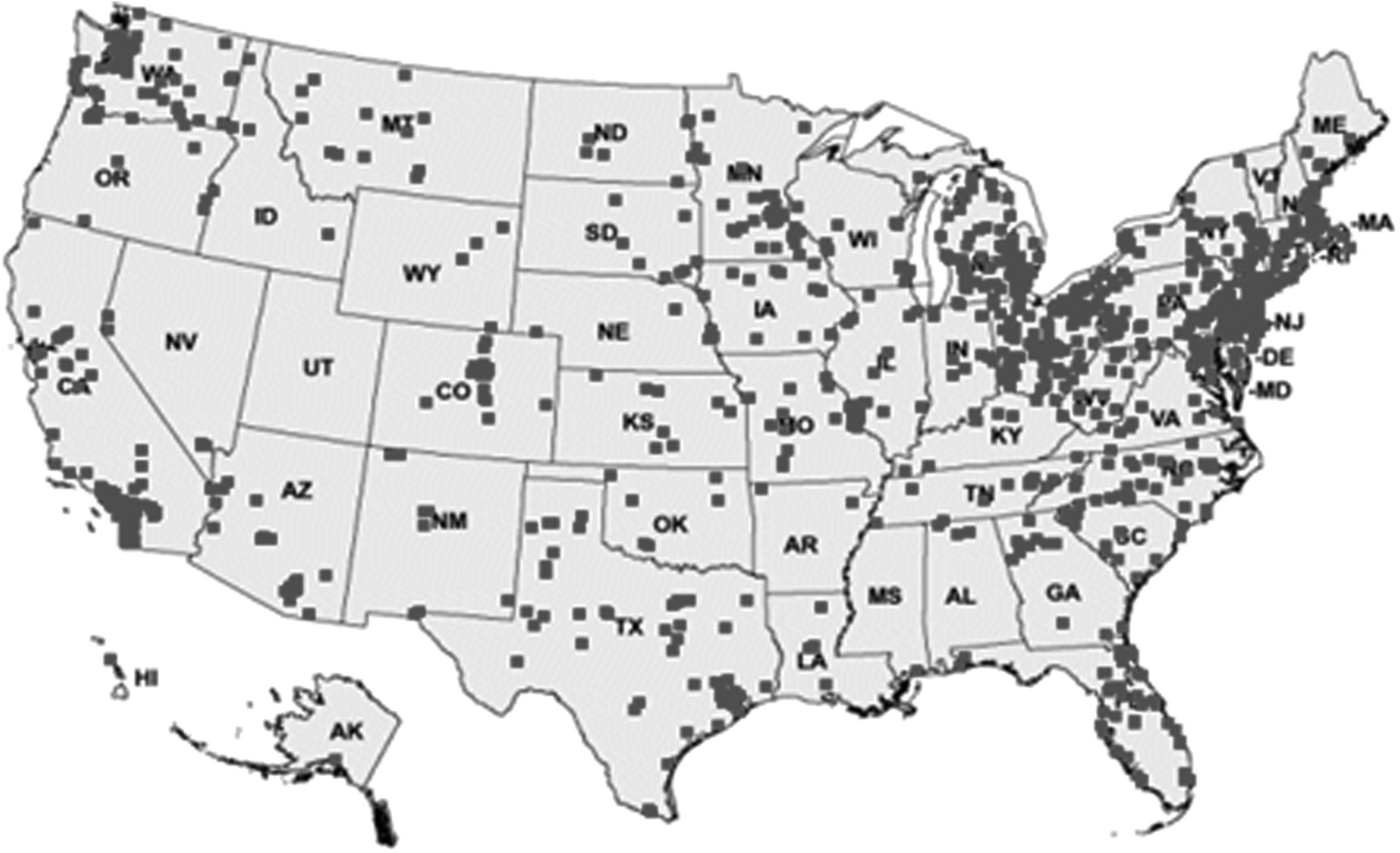
Distribution of ZIP Codes for NETT Participants. Number of ZIP codes=1,128.NETT: National Emphysema Treatment Trial.

Environmental justice is usually defined in terms of differential exposure and differential susceptibility. As we studied an already vulnerable population, we could not assess differential susceptibility in our study. However, using the pathways illustrated in Figure 4, we can see how the presence of differential exposure in our study could relate to differential susceptibility in a healthy but otherwise similar population. Social epidemiologists have postulated that area-level factors exert independent effects on health outcomes.²⁰ Area-level indicators of SES may represent environmental factors such as safety, crowding, availability of healthy food sources, and a sense of community. One or both of these factors could influence differential air pollution exposure risk and differential susceptibility. Those with a lower area-level SES may also be more likely to experience disproportionately higher levels of ambient air pollution exposures due to closer residential proximity to high traffic roadways and industrial sites.^1,3,6

FIG. 4.

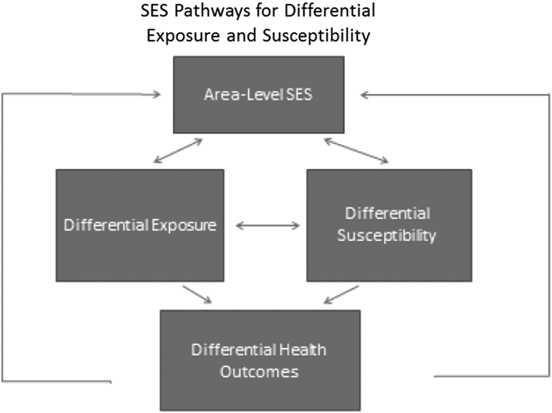
Area-level SES pathways for differential exposure and susceptibility. SES: socioeconomic status.

Comparing our findings to other studies, we found similarities in terms of overall conclusions. Studies by Marshall et al. and Su et al. reported a disproportionate burden of air pollution exposure among lower-income groups.^21,22 A study by Young et al. described differential hazardous air pollution (HAP) exposures with respect to urbanization and neighborhood-level SED, reporting increasing exposure hazards with increasing levels of SED.²³ Despite similar findings, several of the existing studies have focused on the relationship between SES and proximity to hazardous sites and facilities rather than with summary measures of exposure.⁶ In addition, these studies have tended to focus on relatively small geographic areas and disparate group level variables (e.g., census tract), thereby making direct comparisons problematic.

Strengths

Our measure of air pollution exposure was particularly well-suited for this type of study. Typically, spatial autocorrelation is a limitation that is often present in other environmental studies. Air pollution data are particularly subject to this limitation since measures of air quality in nearby communities are not independent of each other. The term spatial autocorrelation in the context of air pollution can be aptly described with the statement “everything is related to everything else, but near things are more related than distant things.”²⁴ Failure to account for this spatial autocorrelation would bias the results by assuming independence in air pollution values when in fact there is not. Our study, which relies on kriged air pollution data, is not subject to this limitation. The kriging methodology is highly dependent on the spatial autocorrelation structure in the data for its prediction or interpolation of air pollution values.^25,13,24 Secondly, we chose to evaluate air pollution exposure with a cumulative rather than a mean value. Using a cumulative measure allowed us to take into account all the daily exposure data as well as capture ranges of low to high exposure concentrations. Relying strictly on a mean value would mask some of the extreme values especially since we are dealing with several years' worth of pollution data. Lastly, the large geographic area covered by the NETT study participants also allows for the generalizability of our findings to populations across the U.S.

Limitations

Although we observed an association between area-level SES and air pollution exposure, we could not assess a similar relationship between individual measures of SES and differential air pollution exposure. Since our exposure was obtained at the ecological level, we could not include individual level measures of SES in our regression analyses. However, since ambient pollutant concentrations were kriged to the centroid of the ZIP code, assessing the relationship between individual-level SES and ZIP code-level concentrations could have been subject to considerable bias. The largely small cluster sizes, ranging from one to three, may have not been representative of the individuals residing within that ZIP code. Since our sample population tended to be largely Caucasian, older, and male, it is likely that their individual-level SES characteristics could have differed considerably from others in their ZIP codes.

As stated previously, much of the literature on environmental justice has been based on ecological or aggregate data. Dependence on ecological data to assess evidence of differential exposure or susceptibility limits one's ability to extrapolate results to the individual level. Control for confounding is also difficult when dealing with purely ecological data, since adjusting for confounders in group level data can be subject to bias or misspecification.²⁶ Confounders at the group-level may not be confounders when examined at the individual-level and the examination of individual-level variables as confounders or effect modifiers cannot be evaluated in strictly ecological studies.²⁷ Employing two separate measures of SES in our study would have permitted the multilevel specification of individual and contextual effects on differential exposures.

One important limitation associated with using ZCTAs to evaluate ZIP code-specific SES characteristics for NETT participants is that although they share the same designation, there is no clear spatial correlation between ZCTAs and ZIP codes.¹⁶ In addition, there are several pitfalls in utilizing ZIP codes as geographical units of analyses. ZIP code boundaries can overlap, be included within other ZIP codes or may be discontinued or newly created over time.²⁸ They can also encompass vast geographical areas and have an average population of approximately 30,000. The development of ZCTA codes as Census groupings arose as a result of the increased use of ZIP codes by public health researchers and investigators.^15,28 ZCTA codes, unlike ZIP codes, are restricted to Census block groups (average population: 1,000).²⁸ In terms of our study, there is potentially significant spatial mismatch in the individuals selected and their representation within the given ZIP code. It is possible that they may reside in an area assigned one ZCTA code but may actually have a different ZIP code. Area-level SES designations may then be inaccurate for these individuals.

The lack of racial/ethnic diversity in our sample did not allow us to assess racial disparities in exposure. Although important, racial and SES inequalities are not strictly functions of one another. Much of the literature on social disparities emphasizes the importance of distinguishing between SES- and racial-related health disparities.²⁹ It has been demonstrated that racial minorities are often at increased risk of adverse health outcomes and higher ambient exposures.^{30,31,32,33,34,35,36} They are also often more likely to have a lower SES.³¹ However, studies have shown that SES and race have independent effects on health outcomes and employing one as a proxy for another may be an inadequate analytic choice.²⁹

Although not the aim of our analyses, we could not infer a causal relationship between SES and differential air pollution exposure. It is often difficult to determine which preceded which—environmental hazards or vulnerable populations. Since region of residence is a non-random selection and land values are typically lower in areas with a greater preponderance of manufacturing plants and waste treatment facilities, it is possible that those from a lower SES would live in areas that contain more of these environmental hazards.³⁰ It is also possible that noxious facilities may be driven away from affluent neighborhoods into poorer areas.³⁷

Another limitation of our study is the lack of information on personal exposures. For this research, we relied on kriged ambient air pollutant concentrations as proxies for personal exposure. Spatial heterogeneity in exposure could have impacted how closely these ambient concentrations correlated with personal exposures. In our study however, this limitation may not be as significant since the heterogeneity in the distribution of ambient pollutant exposure varies greatly by pollutant type. Specifically, PM_2.5 has been shown to have a rather uniform distribution in urban areas due to the predominant influence of small, long-range transport particles.³⁸ This is particularly applicable to our study as our sample was largely urban. Like PM_2.5, ozone has also been shown to have a homogenous distribution over large areas.³⁹ Thus, this limitation may be relatively minor within our sample population.

Lastly, our analyses did not consider the potential multiplicative or additive effects of multiple pollutants. Bivariate correlations revealed a moderate association between ozone and PM_2.5. However, simultaneous consideration of both pollutants in our model would have been inappropriate, as the availability of pollution data was not equal for both pollutants. Ozone data were available from 1998–2003, whereas PM_2.5 were only available from 1999–2003. The disparity in the duration of exposure between pollutants would have complicated controlling for possible interactive effects.

Conclusion

The implications of our study are multifold. We found evidence of an environmental justice equity issue in a vulnerable population. This differential pollutant exposure was shown to be strongly associated with area-level SES. Our study which utilized area-level SES descriptors, over a large geographical area, may enable researchers to more readily compare findings and results. Investigators may also consider applying a similar air pollution kriging methodology in the secondary analysis of health studies with large geographical cohorts. The availability of air pollution data from monitoring databases readily allows for the assessment of differential ambient air pollution in geographically diverse study populations. Specifically, our results speak more directly in support of environmental inequality rather than environmental justice. Characterizing whether this inequality is socially unjust is less clear and subject to further research.

Footnotes

Author Disclosure Statement

The author has no conflicts of interest or financial ties to disclose.

References

Freeman

. “Distribution of Environmental Quality.” In AV Kneese and BT Bower. Environmental Quality Analysis: Theory and Method in the Social Sciences. (Johns Hopkins Press, 1972), 243–278.

Gelobter

Michel

. “Toward a Model for Environmental Discrimination: How Environmental Laws Discriminate Against Low-Income and Minority Communities.” In Bryant and Moohai. Race and the Incidence of Environmental Hazards (1992).

UCC (United Church of Christ). Toxic Wastes and Race in the United States: A National Report on the Racial and Socio-Economic Characteristics of Communities with Hazardous Waste Sites. (United Church of Christ, Commission for Racial Justice, 1987).

Brochu

, et al. “Particulate Air Pollution and Socioeconomic Position in Rural and Urban Areas of the Northeastern United States,”. American Journal of Public Health, 101(2011): S224–S230.

Miranda

, et al. “Making the Environmental Justice Grade: The Relative Burden of Air Pollution Exposure in the United States,”. Int J Environ Res Public Health, 8(2011): 1755–71.

Perlin

, et al. “Distribution of Industrial Air Emissions by Income and Race in the United States: An Approach Using the Toxic Release Inventory,”. Environ Sci Technol, 29(1995): 69–80.

Krieger

, et al. “Painting a True Picture of US Socioeconomic and Racial/Ethnic Health Inequalities: The Public Health Disparities Geocoding Project,”. Am J Public Health, 95(2005): 312–323.

Havard

, et al. “Traffic-related Air Pollution and Socioeconomic Status: Spatial Autocorrelation Study to Assess Environmental Equity on a Small-Area Scale,”. Epidemiology, 20(2009): 223–230.

The National Emphysema Treatment Trial Research Group. “Rationale and Design of The National Emphysema Treatment Trial: A Prospective Randomized Trial of Lung Volume Reduction Surgery. The National Emphysema Treatment Trial Research Group,”. Chest, 116(1999): 1750–61.

10.

Wood

and DeCamp

. “The National Emphysema Treatment Trial: A Paradigm for Future Surgical Trials,”. Ann Thorac Surg, 72(2001): 327–9.

11.

Criner

, Sternberg

. “National Emphysema Treatment Trial: The Major Outcomes of Lung Volume Reduction Surgery in Severe Emphysema,”. Proc Am Thorac Soc, 5(2008): 393–405.

12.

Lutz

David

. AQS Basics: What Data Are in the AQS?. EPA.gov (June 2002). [Cited: June 30, 2011.] <http://www.epa.gov/ttn/airs/airsaqs/manuals/AQS%20Basics.pdf>.

13.

Liao

, Peuquet

, et al. “GIS Approaches for the Estimation of Residential-Level Ambient PM Concentrations,”. Environ Health Perspect, 114(2006): 1374–80.

14.

U.S. Census Bureau. American Fact Finder, Census 2000 Summary File 3 (SF3). (2002).

15.

—. Census 2000 ZIP Code Tabulation Areas Technical Documentation. Census.gov. <http://www.census.gov/geo/ZCTA/zcta_tech_doc.pdf>.

16.

Grubesic

and Matisziw

. “On the Use of ZIP Codes and ZIP Code Tabulation Areas (ZCTAs) for the Spatial Analysis of Epidemiological Data,”. 2006, Int J Health Geogr, 5(2006): 58–73.

17.

Adams

, Ryan

and White

. “How Accurate Are Townsend Deprivation Scores as Predictors of Self-reported Health? A Comparison with Individual Level Data,”. J Public Health, 27(2004): 101–106.

18.

Morris

, Carstairs

. “Which Deprivation? A Comparison of Selected Deprivation Indexes,”. J Public Health Med, 13(1991): 318–26.

19.

Pan

Wei

. “Akaike's Information in Generalized Estimating Equations,”. Biometrics, 57(2001): 120–125.

20.

Kawachi

and Berkman

. Neighborhoods and Health. (Oxford University Press, 2003).

21.

, et al. “Inequalities in Cumulative Environmental Burdens among Three Urbanized Counties in California,”. Environmental International, 40(2012): 79–87.

22.

Marshall

. “Environmental Inequality: Air Pollution Exposures in California's South Coast Air Basin,”. Atmospheric Environment, 42(2008): 5499–5503.

23.

Young

, et al. “Differential Exposure to Hazardous Air Pollution in the United States: A Multilevel Analysis of Urbanization and Neighborhood Socioeconomic Deprivation,”. Int J Environ Res Public Health, 9(2012): 2204–25.

24.

Jerrett

, Gale

, and Kontgis

. “Spatial Modeling in Environmental and Public Health Research,”. Int J Environ Res Public Health, 7(2010): 1302–1329.

25.

Legendre

and Fortin

. “Spatial Pattern and Ecological Analysis,”. Vegetatio, 80(1989): 107–38.

26.

Greenland

. “Ecologic versus Individual-Level Sources of Bias in Ecologic Estimates of Contextual Health Effects,”. Int J Epidemiol, 30(2001): 1343–50.

27.

Diez-Roux

Ana

. “Investigating Neighborhood and Area Effects on Health,”. Am J Public Health, 91(2001): 1789–1789.

28.

Krieger

, et al. “Zip Code Caveat: Bias Due to Spatiotemporal Mismatches between ZIP Codes and US Census Defined Geographic Areas—The Publich Health Disparities Geocoding Project,”. Am J Public Health, 92(2002): 1100–1102.

29.

O'Neill

, et al. “Health, Wealth, and Air Pollution: Advancing Theory and Methods,”. Environ Health Perspect, 111(2003).

30.

Brown

. “Race, Class, and Environmental Health: A Review and Systematization of the Literature,”. Environ Res, 69(1995): 15–30.

31.

Gwynn

and Thurston

. “The Burden of Air Pollution: Impacts Among Racial Minorities,”. Environ Health Perspect, 104(Suppl 4, 2001): 501–6.

32.

Krieger

, et al. “Geocoding and Monitoring of US Socioeconomic Inequalities in Mortality and Cancer Incidence: Does the Choice of Area-Based Measure and Geographic Level Matter? The Public Health Disparities Project,”. Am J Epidemiol, 156(2002): 471–482.

33.

Charafeddine

and Boden

. “Does Income Inequality Modify the Association Between Air Pollution and Health?,”. Environ Res, 106(2008): 81–88.

34.

Jerrett

, et al. “Do Socioeconomic Characteristics Modify the Short Term Association Between Air Pollution and Mortality? Evidence from a Zonal Time Series in Hamilton, Canada,”. J Epidemiol Community Health, 58(2004): 31–40.

35.

Deguen

and Zmirou-Navier

. “Social Inequalities Resulting from Health Risks Related to Ambient Air Quality—A European Review,”. European Journal of Public Health, 20(2010): 27–35.

36.

Dominici

, et al. “Revised Analysis of the National Morbidity, Mortality, and Air Pollution Study: Mortality Among Residents of 90 Cities,”. J Toxicol Environ Health A, 68 (2005): 1071–1092.

37.

Downey

. “US Metropolitan-area Variation in Environmental Inequality Outcomes,”. Urban Stud, 44(2007): 953–977.

38.

Burton

, Suh

and Koutrakis

. “Spatial Variation in Particulate Concentration within Metropolitan Philadelphia,”. Environ Sci Technol, 30(1996): 400–7.

39.

Godish

Thad

. Air Quality. (CRC Press, 1997).

40.

Bowen

. “An Analytical Review of Environmental Justice Research: What Do We Really Know?,”. Environ Manage, 29(2002): 3–15.