Methods for Monitoring Trends in the Incidence of Foodborne Diseases: Foodborne Diseases Active Surveillance Network 1996

Abstract

Foodborne illnesses are a substantial health burden in the United States. The Foodborne Diseases Active Surveillance Network (FoodNet) is the principal foodborne disease component of the Centers for Disease Control and Prevention's Emerging Infections Program. FoodNet is a collaborative project among Centers for Disease Control and Prevention, Emerging Infections Program sites, the U.S. Department of Agriculture, and the U.S. Food and Drug Administration. One of FoodNet's main objectives is to monitor changes in the incidence of selected foodborne pathogens. In 1996, FoodNet began active, population-based surveillance for laboratory-diagnosed cases of Campylobacter, Listeria, Salmonella, Shiga toxin–producing E. coli O157, Shigella, Vibrio, and Yersinia infection. Surveillance for cases of Cryptosporidium and Cyclospora infection was added in 1997 and surveillance for non-O157 Shiga toxin–producing E. coli was added in 2000. From 1997 to 2008, the FoodNet surveillance population increased, primarily through the addition of new sites. The increase in the number of FoodNet sites and the size of the population under surveillance as well as the variation in the incidence of infections among sites posed challenges in the selection of the most appropriate method to monitor changes in incidence. To account for variation introduced by changes in population size, a main-effects, log-linear Poisson (negative binomial) regression model was adopted to estimate the magnitude of changes in the incidence of pathogens by comparing current year incidence to reference periods. The article explains how FoodNet uses the negative binomial model to examine changes in incidence over time, describes the reference periods used, explains the graphics used to display results, and discusses future directions in the analysis of trends over time.

Introduction

F oodborne infections are an important public health problem in the United States (Mead et al., 1999). While advances in technology, regulation, and education over the past century have improved the safety of our food supply, growth of mass production, distribution, and importation of food continues to create new challenges (Allos et al., 2004). To monitor the effectiveness of control efforts, measuring change over time is essential.

The Foodborne Diseases Active Surveillance Network (FoodNet), an active, population-based sentinel surveillance system, has made a major contribution to efforts to improve food safety in the United States. FoodNet provides regulatory agencies, industry, consumer groups, and public health personnel with more precise information on the burden and trends in foodborne diseases than was previously available. Each year, FoodNet provides the most up-to-date information available on trends in selected foodborne diseases. These data are used to prioritize and evaluate food safety interventions and to monitor progress toward national health objectives (Scallan, 2007).

When established in 1996, the FoodNet surveillance area included five sites with a population of 14.3 million persons. From 1996 to 2004, counties and states were added to the surveillance area, and the population under surveillance tripled, to 46.0 million persons in 10 sites in 2008. The expansion of the FoodNet surveillance area and the variation in incidence among FoodNet areas that joined the surveillance system at different times, presented epidemiologic and statistical challenges in the evaluation of trends. To account for variation introduced by changes in population size, in 2001, a main-effects, log-linear Poisson (negative binomial) regression model was adopted to estimate the magnitude of changes in the incidence of pathogens by comparing current year incidence with a reference period. This article explains the reasons for selecting this model, describes implementation, compares the use of different reference periods, describes the graphics selected to display results, and discusses potential future directions in the analysis of trends.

FoodNet and Active Surveillance

FoodNet is a collaborative program that includes the Centers for Disease Control and Prevention (CDC), the U.S. Department of Agriculture's Food Safety and Inspection Service, the U.S. Food and Drug Administration, and selected state health departments in Emerging Infection Program sites (Jones et al., 2007). Monitoring trends in the burden of certain foodborne illnesses in the United States over time is one of FoodNet's primary objectives; the others are to determine the burden of foodborne illness, to attribute that burden to specific foods and settings, and to disseminate information that can be used to develop interventions to reduce the burden of foodborne illness. FoodNet data are also used to monitor progress toward national Healthy People objectives. (Scallan, 2007).

When established in 1996, FoodNet included the states of Minnesota and Oregon as well as selected counties in California (Alameda and San Francisco), Connecticut (Hartford and New Haven), and Georgia (Clayton, Cobb, DeKalb, Douglas, Fulton, Gwinnett, Newton, and Rockdale). From 1997 to 2004, the FoodNet surveillance area expanded several times to ultimately include the entire states of Connecticut, Georgia, Maryland, Minnesota, New Mexico, Oregon, and Tennessee, as well as selected counties in California, Colorado, and New York (Table 1).

Table 1.

Expansion of Surveillance Area of Foodborne Diseases Active Surveillance Network, by Year, 1996–2008

		Year
State	County	1996	1997	1998	1999	2000	2001	2002	2003	2004	2005	2006	2007	2008
California	Original counties (Alameda and San Francisco)	•	•	•	•	•	•	•	•	•	•	•	•	•
	Additional county (Contra Costa)					•	•	•	•	•	•	•	•	•
Colorado	Original counties (Adams, Arapahoe, Denver, Douglas, and Jefferson)						•	•	•	•	•	•	•	•
	Additional counties (Boulder and Broomfield)							•	•	•	•	•	•	•
Connecticut	Original counties (Hartford and New Haven)	•	•	•	•	•	•	•	•	•	•	•	•	•
	Remainder of state			•	•	•	•	•	•	•	•	•	•	•
Georgia	Original counties (Clayton, Cobb, Dekalb, Douglas, Fulton, Gwinnett, Newton, and Rockdale)	•	•	•	•	•	•	•	•	•	•	•	•	•
	Additional counties (Barrow, Bartow Carroll, Cherokee, Coweta, Fayette, Forsyth, Henry, Paulding, Pickens, Spalding, and Walton)		•	•	•	•	•	•	•	•	•	•	•	•
	Remainder of state				•	•	•	•	•	•	•	•	•	•
Maryland	Original counties (Anne Arundel, Baltimore, Baltimore City, Carroll, Harford, and Howard)			•	•	•	•	•	•	•	•	•	•	•
	Additional counties (Montgomery and Prince George's)						•	•	•	•	•	•	•	•
	Remainder of state							•	•	•	•	•	•	•
Minnesota	All counties	•	•	•	•	•	•	•	•	•	•	•	•	•
New Mexico	All counties									•	•	•	•	•
New York	Original sites (Genesee, Livingston, Monroe, Ontario, Orleans, Wayne, and Yates)			•	•	•	•	•	•	•	•	•	•	•
	Additional counties (Albany, Columbia, Greene, Montgomery, Rensselaer, Saratoga, Schenectady, and Schoharie)				•	•	•	•	•	•	•	•	•	•
	Additional counties (Erie, Niagara, and Wyoming)							•	•	•	•	•	•	•
	Additional counties (Allegany, Cattaraugus, Chautauqua, Chemung, Schuyler, Seneca, Steuben, Warren, and Washington)								•	•	•	•	•	•
	Additional counties (Clinton, Delaware, Essex, Franklin, Fulton, Hamilton, and Otsego)									•	•	•	•	•
Oregon	All counties	•	•	•	•	•	•	•	•	•	•	•	•	•
Tennessee	Original counties (Cheatham, Davidson, Dickson, Hamilton, Knox, Robertson, Rutherford, Shelby, Sumner, Williamson, and Wilson)					•	•	•	•	•	•	•	•	•
	Remainder of state								•	•	•	•	•	•

FoodNet conducts population-based active surveillance for laboratory-confirmed infections caused by seven bacterial pathogens (Campylobacter, Listeria monocytogenes, Salmonella, Shiga toxin–producing E. coli O157 [since 2000, other Shiga toxin–producing E. coli serogroups], Shigella, Vibrio, and Yersinia species other than Y. pestis) and two parasitic pathogens (Cyclospora and Cryptosporidium, for which surveillance started in 1997). Surveillance is conducted in collaboration with the more than 650 clinical laboratories serving the population under surveillance using standard case definitions and comparable data collection methods. FoodNet personnel at each site actively contact all of these clinical laboratories regularly to ascertain laboratory-confirmed cases (Hardnett et al., 2004). For each case of infection with one of the pathogens monitored, we collect information including the date of onset of illness, the state and county where the patient with the reported infection resides, age of the patient, whether the patient traveled in the 7 days before onset of symptoms, and whether the case was outbreak associated.

Modeling Trends over Time

Before 2001, only data from the original 5 FoodNet surveillance sites were used in the evaluation of trends, thus not making full use of FoodNet data. In 2001, we began to use a negative binomial regression model to evaluate trends, because this model allows the use of all data from all sites and can account for changes in the surveillance area. That said, the increase in population under surveillance with respect to time implies that rates for earlier time periods are estimated with less precision than for later periods. We considered using a Poisson regression model, also known as a log-linear model, a type of analysis that has traditionally been used to model rate data (Frome, 1983). Poisson regression is an optimal approach when there is no overdispersion of the data and when there are no excess zeros in the data. However, state-to-state and county-to-county variations in incidence in FoodNet produce both overdispersion and excess zeros in the surveillance data—that is, to varying degrees, clustering of cases in time and space is characteristic of FoodNet data. A negative binomial model is an extension of the Poisson regression model that accommodates this type of variation (Pedan, 2001). Thus, it explicitly controls for site-to-site incidence variation while estimating changes in incidence.

Using the negative binomial model, each year we estimate the change in incidence between the most recent year and the reference period of interest. Figure 1 is an example of the SAS (v.9.2, SAS Institute Inc, Cary, NC) code used to run the model. First, we create a dataset aggregated by pathogen (“PATHOGEN,” in Fig. 1), year the infection occurred (“YEAR”), and year in which each county or state entered FoodNet (“STATE_ENTYEAR”). For each combination of these variables, we sum the number of cases of infections reported (“COUNT”), determine the corresponding population based on U.S. Census population estimates, and calculate the log of the population estimate (“LOGPOPULATION”). Using the PROC GENMOD procedure in SAS we fit the negative binomial regression model to this dataset. We specify the distribution of the “COUNT” as negative binomial, and the “link” function as “log.” The natural log of the mean of the negative binomial distributed dependent variable is defined by a linear combination of two predictor variables; changes in incidence are measured by the effect of “YEAR” while “STATE_ENTYEAR,” as defined above, controls for changes in surveillance area and site-to-site variation in incidence. A set of estimate statements are used to create the different reference periods of interest.

FIG. 1.

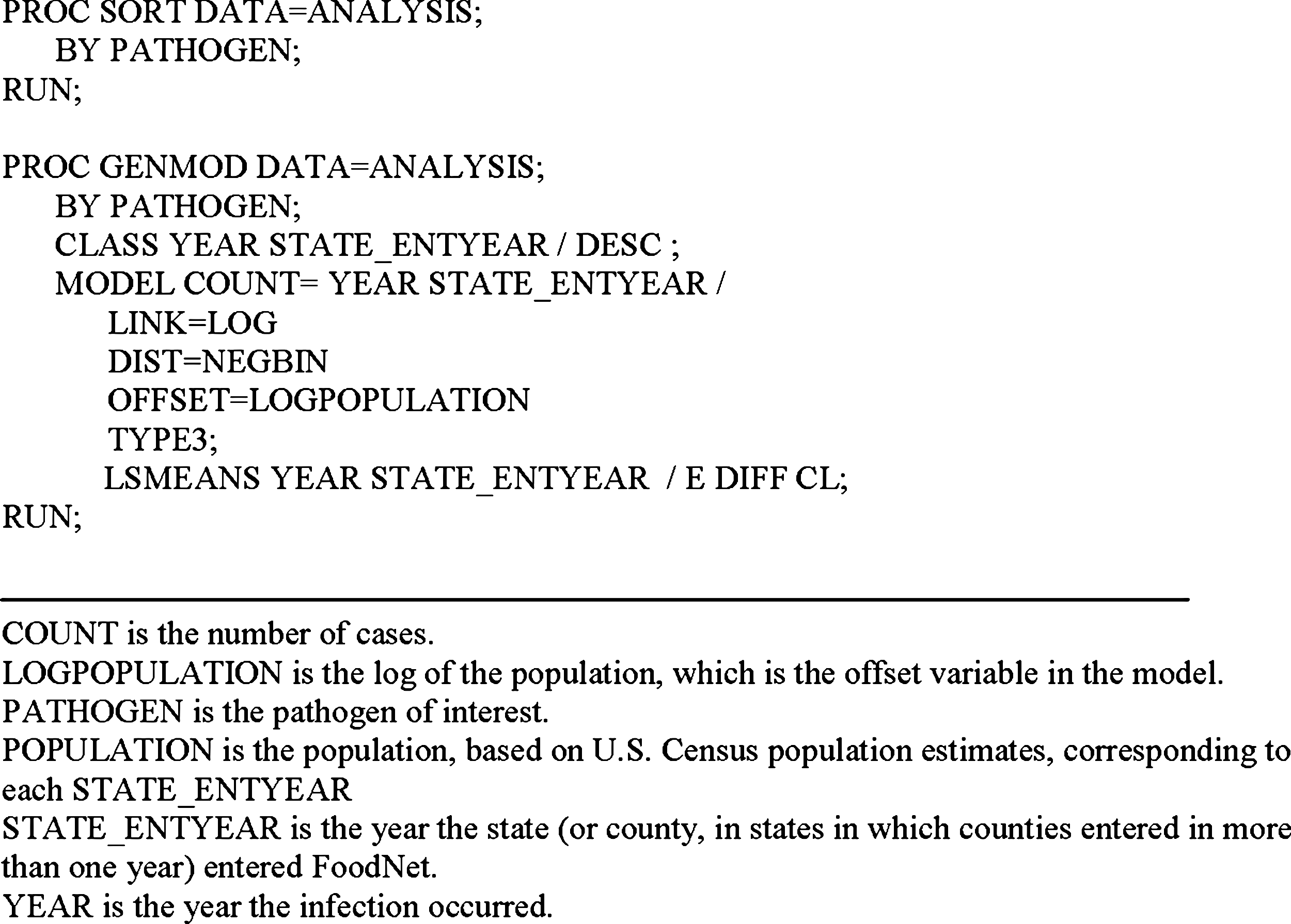
SAS code used to run the negative binomial regression model using Foodborne Diseases Active Surveillance Network data.

Reference Periods

Selection of the most appropriate reference period for examination of trends in FoodNet data is challenging, both because of the growth of FoodNet and because the best baseline against which to measure future changes varies depending on what is being assessed. We have used several reference periods. From the introduction of the negative binomial model in 2001 through 2004, we used the first year of FoodNet surveillance (1996) as the reference period (CDC 2001, 2002, 2003, 2004; Scallan, 2007). In 2005, to better account for fluctuations in reported incidence rates in FoodNet's first years, we started using the used the average annual incidence from the first 3 years (2 years for Cryptosporidium) of surveillance as the reference period (CDC, 2005). In 2007, we introduced an additional reference period—the average annual incidence for the 3 years preceding the year of interest (CDC, 2007).

Using the comparison periods, we report the estimated change in incidence for the most recent year of data using a relative rate (RR) and a 95% confidence interval. Percent change in incidence and corresponding confidence intervals are calculated by subtracting 1 from the RRs and confidence intervals and multiplying by 100. To display the information we use two graphing schemes (described in the next section). As an example, Table 2 shows the RRs and percent changes for 2008 for each of three reference periods: (1) 1996 (the first year of surveillance), (2) 1996–1998 (the first 3 years of surveillance), and (3) 2005–2007 (the 3 years immediately preceding the year of the report). As illustrated by the tighter confidence intervals in Table 2, the use of 1996–1998 as the reference period provides for a more precise estimate of the reference rate and thus results in more stable RR estimates than 1996 alone. Using the 3 years preceding the year of the report as an additional reference period provides a way to examine recent changes in incidence; as FoodNet surveillance moves into its second decade, the ability to make formal comparisons to a period more recent than the start of surveillance becomes increasingly important.

Table 2.

Relative Rates of Laboratory-Diagnosed Cases of Infection Using Three Reference Periods in a Negative Binomial Model, Foodborne Diseases Active Surveillance Network, United States, 2008

	Reference period
	1996 (first year)		1996–1998 (first 3 years)		2005–2007 (preceding 3 years)
Pathogen	Relative rate	95% CI	Relative rate	95% CI	Relative rate	95% CI
Campylobacter	0.69	(0.62, 0.77)	0.68	(0.64, 0.74)	0.99	(0.93, 1.05)
STEC O157	0.76	(0.56, 1.03)	0.75	(0.61, 0.93)	1.02	(0.86, 1.20)
Listeria	0.68	(0.50, 0.92)	0.64	(0.51, 0.80)	1.01	(0.83, 1.23)
Salmonella	0.90	(0.80, 1.01)	0.97	(0.90, 1.04)	1.06	(1.00, 1.12)
Shigella	0.48	(0.28, 0.83)	0.60	(0.42, 0.86)	0.98	(0.75, 1.29)
Vibrio	2.18	(1.31, 3.66)	1.52	(1.13, 2.06)	1.05	(0.84, 1.32)
Yersinia	0.49	(0.36, 0.66)	0.52	(0.42, 0.66)	1.02	(0.83, 1.25)

CI, Confidence interval; STEC, Shiga toxin–producing Escherichia coli.

Graphical Presentation of Trends over Time

Figure 2 is a graphical representation of the RRs of infection with five pathogens under FoodNet surveillance from the start of FoodNet through 2008, as compared with the 1996–1998 reference period. It includes the four pathogens with a Healthy People 2010 objective as well as Vibrio. Years are on the X-axis, and RRs are on the Y-axis on a logarithmic scale. A reference line is displayed at RR = 1 to allow the reader to easily discern the direction of change for any year, as compared with the 1996–1998 period. Points above the reference line indicate increases in incidence; points below indicate decreases. This graph does not indicate whether incidence changes were statistically significant. This graphic allows easy comparison of multiple years and pathogens. For example, for Campylobacter infection, after an initial decline in the early years of FoodNet surveillance, the RR since 2001 has changed little. In contrast, rates of Vibrio infection in FoodNet were lower than in the reference period until 2001 but have since been higher.

FIG. 2.

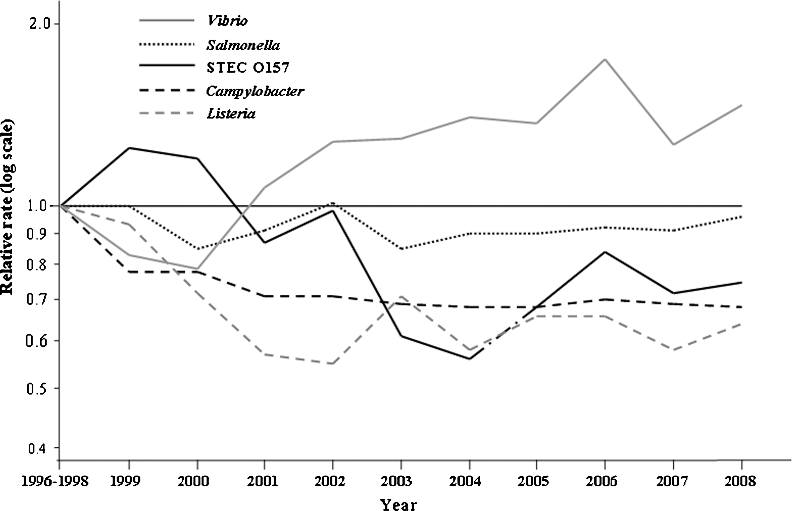
Relative rates of laboratory-diagnosed cases of infection with Vibrio, Salmonella, Shiga toxin–producing Escherichia coli (STEC) 0157, Campylobacter, and Listeria, compared with 1996–1998 period—Foodborne Active Surveillance Network, United States, 1996–2008. The position of each line indicates only the relative change in the incidence of that pathogen compared with the years 1996–1998. The actual incidences of these infections cannot be determined from this graph.

Figure 3 provides a graphic display of rate comparisons using the more recent reference period; it displays the percent change in a given year (in this case 2008) compared with the average annual incidence over the preceding 3 years. Pathogens are displayed on the X-axis and percent changes on the Y-axis. A reference line is displayed at percent change = 0. In contrast to Fig. 2, this graphic also displays confidence intervals for the estimates of change, allowing the reader to easily ascertain if the change in recent incidence is statistically significant. In this example, only the change in Salmonella incidence is significant.

FIG. 3.

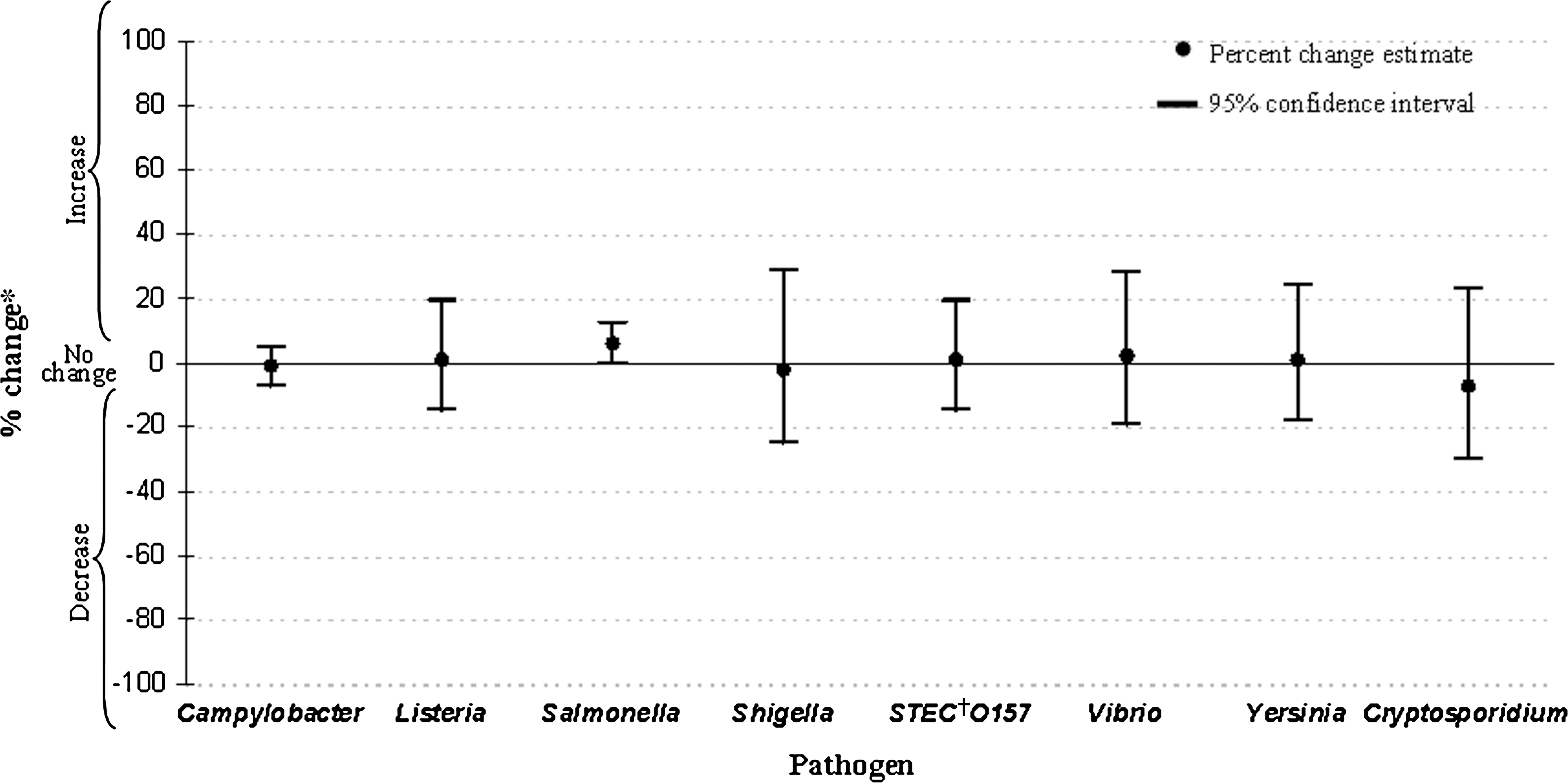
Percent change in the incidence of laboratory-confirmed bacterial infections in 2008 compared with the preceding 3 years (2005–2007), Foodborne Diseases Active Surveillance Network, United States. *No significant change = 95% confidence interval is both above and below the no change line; significant increase = estimate and entire 95% confidence interval are above the no change line; significant decrease = estimate and entire 95% confidence interval are below the no change line. ^†Shiga toxin–producing Escherichia coli.

Discussion

We have presented the rationale and methods for the approaches currently used to evaluate and report trends in FoodNet surveillance data, the reference periods used for comparison with current surveillance data, and the graphs used to display these results. This detailed exposition of these methods complements FoodNet's annual presentation of current data on the incidence of several important infections transmitted commonly through food. Understanding these methods may be useful to stakeholders, including public health and food regulatory authorities, consumer advocacy organizations, the food industry, and others.

To evaluate trends, we selected the negative binomial model, an extension of Poisson regression that allows for the overdispersion and excess zeroes seen in FoodNet data. This model is straightforward to use, its results are readily interpretable, and it adequately accounts for the changing FoodNet surveillance area and the variation in incidence both from site to site and within sites. The model implicitly assumes that the disease process, as described by the main effects of year and location, is valid for those combinations of year and state that were not observed. We have validated this assumption to the extent that subset analysis of the data allows. For some of the lower incidence pathogens with little variation in incidence by site—Listeria is a good example—both the basic log-linear Poisson model and the negative binomial Poisson model fit well. However, the negative binomial model is preferable, because it provides greater flexibility than the basic log-linear Poisson model for dealing with overdispersion and excess zeroes that could occur (Pedan, 2001). We changed from a single year to a 3-year baseline reference period because this baseline led to more stable and precise RR estimates (CDC, 2005). The estimates obtained in the regression procedure for each pathogen are based on the counts for each site by year, meaning that, as new data are accrued, the estimates of effect for both site and year are modified. The accrual of new data changes the estimates of both current and historical year effects and, therefore, the associated RRs that are reported. However, sufficient data have now been accrued that these fluctuations are trivial. To allow formal comparisons to a recent time period, we added a comparison with the 3 years immediately preceding the year of the report.

We plan to continue exploring descriptions of the FoodNet data based on the negative binomial model and to incorporate useful explorations into future reports. We also continue to explore other methods to supplement our analyses, such as joinpoint regression analysis (http://srab.cancer.gov/joinpoint). Examples of future analyses include the evaluation of trends by age group to determine whether, as has been reported elsewhere, different trends are at play in different segments of the population (Gillespie et al., 2009). Similarly, analysis of trends in travel- and outbreak- related cases might provide additional insight relevant to prevention efforts. Expansion of modeling approaches to adjust for seasonality may allow increased precision of estimates of trends. We will also explore the use of smooth predictors based on time, in addition to the discrete predictors that we currently use, to summarize longer-term patterns of disease incidence.

Conclusion

FoodNet conducts active population-based surveillance for infections commonly transmitted through food and provides unique and timely data on the incidence of and trends in these infections, important information to support decision making regarding food safety. Substantial expansion of the FoodNet surveillance area over time has presented challenges in monitoring changes in incidence over time. This report explains FoodNet's current methods for evaluating and reporting trends and the rationale for choosing those methods. We use a negative binomial model and two comparison periods, one more distant and the other more recent, to evaluate trends in the incidence of infection with pathogens under surveillance in FoodNet. Using both comparison periods provides a more comprehensive picture of changes in incidence of infections with the pathogens of interest than either comparison period alone.

Footnotes

Disclosure Statement

No competing financial interests exist.

References

Allos

, Moore

, Griffin

, Tauxe

. Surveillance for sporadic foodborne disease in the 21st century: the FoodNet perspective. Clin Infect Dis, 2004; 38,Suppl 3:S115–S120.

[CDC] Centers for Disease Control and Prevention. Preliminary FoodNet data on the incidence of foodborne illnesses—selected sites, United States, 2000. MMWR Morb Mortal Wkly Rep, 2001; 50:241–246.

[CDC] Centers for Disease Control and Prevention. Preliminary FoodNet data on the incidence of foodborne illnesses—selected sites, United States, 2001. MMWR Morb Mortal Wkly Rep, 2002; 51:325–329.

[CDC] Centers for Disease Control and Prevention. Preliminary FoodNet data on the incidence of foodborne illnesses—selected sites, United States, 2002. MMWR Morb Mortal Wkly Rep, 2003; 52:340–343.

[CDC] Centers for Disease Control and Prevention. Preliminary FoodNet data on the incidence of infection with pathogens transmitted commonly through food—selected sites, United States, 2003. MMWR Morb Mortal Wkly Rep, 2004; 53:338–343.

[CDC] Centers for Disease Control and Prevention. Preliminary FoodNet data on the incidence of infection with pathogens transmitted commonly through food—10 sites, United States, 2004. MMWR Morb Mortal Wkly Rep, 2005; 54:352–356.

[CDC] Centers for Disease Control and Prevention. Preliminary FoodNet data on the incidence of infection with pathogens transmitted commonly through food—10 states, 2006. MMWR Morb Mortal Wkly Rep, 2007; 56:336–339.

Frome

. The analysis of rates using Poisson regression models. Biometrics, 1983; 39:665–674.

Gillespie

, O'Brien

, Bolton

. Age patterns of persons with campylobacteriosis, England and wales, 1990–2007. Emerg Infect Dis, 2009; 15:2046–2048.

10.

Hardnett

, Hoekstra

, Kennedy

, Charles

, Angulo

. Epidemiologic issues in study design and data analysis related to FoodNet activities. Clin Infect Dis, 2004; 38,Suppl 3:S121–S126.

11.

Jones

, Scallan

, Angulo

. FoodNet: overview of a decade of achievement. Foodborne Pathog Dis, 2007; 4:60–66.

12.

Mead

, Slutsker

, Griffin

, Tauxe

. Food-related illness and death in the united states reply to Dr. Hedberg. Emerg Infect Dis, 1999; 5:841–842.

13.

Pedan

. Analysis of count data using the SAS System. SUGI 26 Proceedings Paper, 2001; 247:1–6.

14.

Scallan

. Activities, achievements, and lessons learned during the first 10 years of the Foodborne Diseases Active Surveillance Network: 1996–2005. Clin Infect Dis, 2007; 44:718–725.

Methods for Monitoring Trends in the Incidence of Foodborne Diseases: Foodborne Diseases Active Surveillance Network 1996–2008