In this article, we describe a novel holonomic soft robotic structure based on a parallel kinematic mechanism. The design is based on the Stewart platform, which uses six sensors and actuators to achieve full six-degree-of-freedom motion. Our design is much less complex than a traditional platform, since it replaces the 12 spherical and universal joints found in a traditional Stewart platform with a single highly deformable elastomer body and flexible actuators. This reduces the total number of parts in the system and simplifies the assembly process. Actuation is achieved through coiled-shape memory alloy actuators. State observation and feedback is accomplished through the use of capacitive elastomer strain gauges. The main structural element is an elastomer joint that provides antagonistic force. We report the response of the actuators and sensors individually, then report the response of the complete assembly. We show that the completed robotic system is able to achieve full position control, and we discuss the limitations associated with using responsive material actuators. We believe that control demonstrated on a single body in this work could be extended to chains of such bodies to create complex soft robots.
Introduction
Soft robotic systems have unique characteristics, such as high deformability and impact resistance, that make them potential alternatives to traditional robots in applications such as mobility in unstructured environments and operation in proximity to humans.1 Unlike in traditional rigid robots, where deformations are sources of error to be avoided, in soft robots the change in geometry is essential to the functioning of the robot.2 Further, deformations are distributed throughout the body in soft robots, unlike in traditional rigid robots where articulation is localized at joints with limited degrees of freedom (DoF).3 Distributed deformations allow soft robots to forgo bearings and joints for articulation, which has the potential to greatly reduce cost and complexity while increasing durability, particularly in dusty or corrosive environments.
The same characteristics that make soft robots interesting also make these systems difficult to design and control.4 To take advantage of the deformations of these bodies, they must be controlled, which requires both sensing and actuation. The large deformations present in soft robotic systems necessitate the use of stretchable state observation sensors whereas the distribution of deformations throughout the body, rather than at discrete joints, complicates the sensor placement problem.5 One simplification we make in this work is the consideration of only discrete points on a soft body. In this scheme, the exact deformation field within the body away from the points is unimportant, and only the deformations of the points relative to one another are considered.
This work demonstrates a holonomic three-dimensional soft robot module, as shown in Figure 1. A single piece of elastomer will naturally have nontrivial compliance in all DoFs. In three-dimensional space, this means that six DoFs are required to fully define the deformation of an elastomer body, and six independent channels of sensing and actuation are required to observe and control the deformation. One potential configuration of sensors and actuators to achieve holonomic control is suggested by the Stewart platform.6 Although there are many solutions to this challenge, we believe that the Stewart platform configuration used in this article is a highly efficient way to position sensors and actuators around a soft body. Our selection of a Stewart platform configuration is motivated by our long-term goal of completely integrating all of the sensing, actuation, and structural elements into a single body. A Stewart-like configuration could use sensors and actuators located on the outer surface of the structure, with no overlapping elements. Both these considerations are extremely important to facilitate manufacturing of an integrated soft system.
Completed soft robotic module with support electronics. Not shown is a power supply and PC hosting the control software and user interface. The robotic structure is the blue and red object at center right. An Arduino used to communicate with the PC is behind and to the left of the robotic structure. Closed-loop current controllers for the SMA actuators are in the foreground at right. The robotic structure consists of two moving rigid plates (blue) connected by a deformable silicone body (red). There are six sensors and six actuators connected between the upper and lower rigid plates. These sensors and actuators are shown in the inset. For a schematic illustration of the robot with components labeled, please refer to Figure 2. SMA, shape memory alloy. Color images available online at www.liebertpub.com/soro
The deformable body at the core of the soft robot module comprised silicone elastomer cast into a spherical shell structure. We selected this geometry to make the stiffness in each DoF comparable. For example, had a solid structure been used, the compressive stiffness would have been at least an order of magnitude higher than the bending stiffness. Acting against this body are six nickel-titanium shape memory alloy (SMA) actuators configured into spring-like coils; the elastomer body and actuators act as an “antagonistic pair.” The actuators are only capable of contracting when actuated, and they require an external restoring force to extend. In this robot module, that force is provided by a combination of the deformable elastomer body at the core of the structure and the other actuators. Conductive composite elastomer-based strain gauges are used to observe the state of the system.
By integrating highly deformable elastomer structures, responsive material actuators, and large deformation strain sensors into a single module, we have created a robotic architecture that can be applied to a wide range of soft robotic applications and structures. In addition to the particular materials selected for this application, other types of deformable bodies, actuators, and sensors could be used in other applications while retaining the same robot topology. In the future, this same basic structure could be used to create dexterous soft robotic limbs from chains of these segments.
In addition to holonomic systems, we believe that the same components and design philosophy could be used to create either over- or under-actuated robotic systems as well. Under-actuated octopus-inspired cable-driven limbs were described by Calisti et al.7 Since control of under-actuated systems is nontrivial, these structures have also seen additional work focused on control.8,9 Bridging the gap between our concept of modular fully actuated structures and under-actuated continuum bodies, fluid-actuated multi-segment limbs were demonstrated by Marchese et al.10,11 We believe that a combination of fully- and under-actuated components will provide the best performance to complex soft robotic systems. Because of this, we see our work as complementing, rather than replacing, the ongoing work on under-actuated soft robots.
Previous Work
The unique characteristics of soft robots come from their material composition, unlike traditional robots where materials are less of a concern than the geometry of the structure. To develop the robotic module described in this article, we have had to not only integrate existing elements but also further develop the state of the art at the component level, particularly in the area of soft sensing, as a part of our integration effort. In our previous work, we demonstrated the control of a single DoF elastomer body by using SMA actuators and liquid metal sensors.12 This work builds on our previous system by increasing the number of DoF, sensors, and actuators, all of which result in significant challenges in reliability and integration. Previous work by other groups has demonstrated controlled motion of a snake-like robot13 and uncontrolled motion in other elastomer systems, such as crawling robots,14 grippers,15 tentacles,16 and actuators in hybrid rigid/soft systems.17 In this work, we expand on what has been published previously by using position observation and feedback in a multi-DoF system to achieve closed-loop control, which we believe is a critical next step to enabling more complex soft robots.
Parallel kinematic systems
The parallel kinematic architecture of the robotic structure we describe in this article was first described by Stewart.6 Over the past five decades, there has been significant research on these parallel kinematic platforms, although most of the fundamental work occurred during the 1980s and 1990s.18 The Stewart platform provides high stiffness and full six DoF motion within a smaller volume than a similarly sized serial kinematic system. For this reason, Stewart platforms have found narrow yet deep success in areas such as full-motion flight simulators and micropositioning systems. Creating a traditional Stewart platform with spherical and universal joints results in a complex assembly with many components. In contrast to a jointed system, a soft system such as the one we present in this work relies on the naturally low stiffness of elastomer components to achieve motion through bending, which results in a more mechanically robust structure with fewer failure modes.
In addition to using traditional actuators, parallel kinematic systems with SMA actuators have been described with two-axis,19 three-axis,20 and six-axis motion.21 Further, two of these approaches were extended into multi-segment chains.21,22 The two major differences between the previous work and the current work are the use of soft sensors for state feedback and highly deformable elastomers for structural elements. Although previous examples of SMA-based systems have demonstrated material state feedback by measuring electrical resistance of the actuator wire, this does not provide information on the configuration of the overall structure. To overcome this limitation, we have added elastomer-based strain sensors to provide measurements of the deformed state of the platform. The previous approaches also rely on a conventional joint or joints. In our work, we eliminate the use of mechanical joints by using deformable structures. This significantly decreases the part count and complexity of the overall design, and it moves the state of the art forward toward integrated soft robotic systems.
Sensors
There are many potential solutions for proprioceptive feedback in soft robotic systems. Our group recently presented a review of planar sensor-embedded structures that we refer to as “sensory skins.”23 Both resistive and capacitive sensors made from a range of materials have been demonstrated. Two common material approaches to making very high deformation electrical conductors are elastomer-based composites24 and liquid metals.25 Liquid metals are very common in the soft robotics literature, and have been used to fabricate a range of soft systems, including keypads,26 curvature,27,28 pressure,29 contact force,30 and multimodal pressure and strain sensors.31,32 Proprioceptive liquid metal sensors embedded in soft actuators have been described, which is a very similar application to what we describe in this work.33–35 In our own previous work, we used liquid metal sensors to measure the state of an SMA-actuated soft robotic system12 and to create modular sensory skins.36
An alternative approach to resistive sensing is to use changes in capacitance to measure strain. Previous elastomer-based capacitive strain sensors have been demonstrated with gold37 and carbon nanotube38 electrodes. Both these approaches may enable smaller capacitive sensors than we constructed in this study, which we believe will facilitate integration of sensing into soft robots and systems with distributed deformations. We chose to employ capacitive conductive composite sensors due to ease of manufacture, robustness, and stability over time. We selected a graphene-based conductive composite as our electrode, which is a class of materials reviewed in Ref.39 In particular, our electrode material was inspired by the work of Kujawski et al.40 However, in the original work, the expanded graphene material was used as a resistive strain sensor, whereas we use it as an electrode in a capacitive sensor. This mitigates the drift and degradation observed when conductive composites are employed as resistors, at the cost of more complex signal conditioning.
Actuators
There are many types of responsive material or soft actuators that could be used in this application, including pneumatics, dielectric elastomers, shape memory materials, hydrogels, and ionic polymer composites.41 A frequently reported type of actuator in the recent soft robotics literature is the pneumatic actuator.42 McKibbon actuators are a commonly used type of pneumatic soft actuator that could directly replace our SMA actuators.43 These alternatives have lower power and energy densities than SMA actuators and require more complex interface hardware consisting of a pressure source and valves. In addition to McKibbon actuators, which are designed to replace traditional pneumatic pistons, using pressure to directly deform soft bodies has also been demonstrated.14,44 In our robotic system, our sensors and actuators are individual components. However, direct integration of liquid-metal-based sensors into actuators has already been demonstrated in McKibbon actuators33 and deformable body pneumatic systems.34,35
Shape memory materials, and particularly alloys that comprised nickel and titanium, have received significant attention45 since the discovery of the shape memory effect by Jackson et al.46 The mechanics behind metallic SMAs have been extensively studied, and many different approaches exist to explain the underlying physical phenomena.47 Metallic SMAs have been used in many applications as actuators for macro-scale48 and micro-scale systems.49 Shape memory materials have been used in soft robots in the form of sheets50 and wires.51 SMAs have been used extensively in mobile soft robotic applications, including in robots inspired by worms,52–54 fish,55 manta rays,56 starfish,57 turtles,58 and in more traditional systems such as underactuated cylinders59 and jumping robots.60 As mentioned in the Introduction, coiled SMA actuators are only capable of producing tension. This poses design challenges not frequently found in traditional actuators. Liang and Rogers presented an analysis of single, passively biased, and antagonistic SMA actuators.61 This basic concept, of using an external force to provide a counter-acting force to the actuator, has been reused in almost all subsequent SMA work.
SMA antagonists fall into the two categories described by Liang and Rogers: passive springs or active SMA actuator pairs. An early example of SMA antagonist pairs was demonstrated by Ikuta et al., who combined multiple SMA actuator pairs into a continuum manipulator for endoscopic surgery.62 This application is very similar to our previous work12 but with rigid components and traditional joints instead of a deformable elastomer body. In this work, we have extended control of deformable bodies into three-dimensional space.
Researchers have had to address the complex thermomechanical control problem inherent in working with SMA. Two approaches have been used: to measure some property, typically resistance, of the SMA actuator to estimate its present internal state, or to measure the displacement output of the actuator. Ikuta et al. demonstrated both methods concurrently, using a material model that was later refined by Majima et al., who demonstrated that measurements of resistance could be used to control SMA-actuated systems.62–65 In our own previous experiments, we found that resistance-based state estimation is highly dependent on loading condition and ambient temperature, resulting in large errors without additional measurements. For this reason, we use direct measurement of actuator displacement in this work.
Designing the shape of the SMA actuators remains a heuristic process, although attempts are being made to provide rigor to the design process. De Aguiar et al. presented a model of coiled SMA actuator performance based on the mechanics of helical springs and a one-dimensional constitutive equation.66 An et al. provided a review of SMA coils from the perspective of providing design rules.67 In designing an SMA actuator, particularly one that will be used with an elastomer antagonist, there are three major criteria that must be considered. First, the actuator must apply enough force in the “on” state to perform the desired motion. Second, the antagonist must have sufficient strength to return the actuator to the desired “off” position, while not being so strong as to interfere with the first objective. Third, when a majority of the actuators are “on” or are still cooling, the antagonist must be sufficiently strong to resist bucking or collapse. In this work, our design process started with the desired size of the finished robotic system, and then considered the minimum, neutral, and maximum lengths of the actuators. Next, we compared stretchability of a handful of samples we manufactured with different wire diameters and coil diameters, where both parameters were constrained by commercially available materials. Finally, we were able to quickly converge on a usable, although not optimal, actuator design. Our experience demonstrates that better actuator and soft system design tools would be beneficial to further developments in this field.
Platform Kinematics
One of the barriers to wider adoption of parallel kinematic systems is the non-linear mathematics that govern the kinematics of the platform. The purpose of the Stewart platform is to achieve full six DoF motion relative to the base platform by using six sensors and six actuators. In our formulation, we consider two different sets of states: a configuration state vector that describes the location of the moving platform relative to the stationary platform, and a length state vector that describes the lengths between nodes on the platforms. We use two sets of states because we want to control the motion of the system in a natural coordinate system with motions such as “move right” or “pitch down,” yet we must observe and actuate the system by using length-based sensors and actuators. We define a configuration vector describing the transformation from the base to the work platform as:
\documentclass{aastex}\usepackage{amsbsy}\usepackage{amsfonts}\usepackage{amssymb}\usepackage{bm}\usepackage{mathrsfs}\usepackage{pifont}\usepackage{stmaryrd}\usepackage{textcomp}\usepackage{portland, xspace}\usepackage{amsmath, amsxtra}\usepackage{upgreek}\pagestyle{empty}\DeclareMathSizes{10}{9}{7}{6}\begin{document}
\begin{align*} { \bf{c}} = { [ {x_1} , {x_2} , {x_3} , {q_r} ,
{q_1} , {q_2} , {q_3} ] ^T} , \tag{1}
\end{align*}
\end{document}
where x1, x2, x3 represent translations in an orthonormal coordinate system \documentclass{aastex}\usepackage{amsbsy}\usepackage{amsfonts}\usepackage{amssymb}\usepackage{bm}\usepackage{mathrsfs}\usepackage{pifont}\usepackage{stmaryrd}\usepackage{textcomp}\usepackage{portland, xspace}\usepackage{amsmath, amsxtra}\usepackage{upgreek}\pagestyle{empty}\DeclareMathSizes{10}{9}{7}{6}\begin{document}
$${ \bf{e}}$$
\end{document} and qr, q1, q2, q3 represent a rotation described in terms of quaternions. All three of the classic rotation representations, Euler angles, direction cosine matrices, and quaternions, appear in the parallel kinematics literature, with no representation being clearly superior to the others. We selected a quaternion representation to eliminate the possibility of gimble lock and to take advantage of computational efficiency. In addition, quaternions can readily be used to describe rotations about the local coordinate system attached to the moving plane. This is useful when the robot is used as a part of a human-in-the-loop system, for example, allowing an operator to request a “pitch up” or “turn left” motion relative to the current location. As with all quaternion formulations, four parameters are used to represent a rotation in three dimensions, necessitating the addition of an auxiliary constraint that the rotation direction be a unit vector:
\documentclass{aastex}\usepackage{amsbsy}\usepackage{amsfonts}\usepackage{amssymb}\usepackage{bm}\usepackage{mathrsfs}\usepackage{pifont}\usepackage{stmaryrd}\usepackage{textcomp}\usepackage{portland, xspace}\usepackage{amsmath, amsxtra}\usepackage{upgreek}\pagestyle{empty}\DeclareMathSizes{10}{9}{7}{6}\begin{document}
\begin{align*}
q_1^2 + q_2^2 + q_3^2 = 1. \tag{2}
\end{align*}
\end{document}
where \documentclass{aastex}\usepackage{amsbsy}\usepackage{amsfonts}\usepackage{amssymb}\usepackage{bm}\usepackage{mathrsfs}\usepackage{pifont}\usepackage{stmaryrd}\usepackage{textcomp}\usepackage{portland, xspace}\usepackage{amsmath, amsxtra}\usepackage{upgreek}\pagestyle{empty}\DeclareMathSizes{10}{9}{7}{6}\begin{document}
$${{ \rm{l}}_{i , j}}$$
\end{document} is the length between the \documentclass{aastex}\usepackage{amsbsy}\usepackage{amsfonts}\usepackage{amssymb}\usepackage{bm}\usepackage{mathrsfs}\usepackage{pifont}\usepackage{stmaryrd}\usepackage{textcomp}\usepackage{portland, xspace}\usepackage{amsmath, amsxtra}\usepackage{upgreek}\pagestyle{empty}\DeclareMathSizes{10}{9}{7}{6}\begin{document}
$$i{ \rm{th}}$$
\end{document} and \documentclass{aastex}\usepackage{amsbsy}\usepackage{amsfonts}\usepackage{amssymb}\usepackage{bm}\usepackage{mathrsfs}\usepackage{pifont}\usepackage{stmaryrd}\usepackage{textcomp}\usepackage{portland, xspace}\usepackage{amsmath, amsxtra}\usepackage{upgreek}\pagestyle{empty}\DeclareMathSizes{10}{9}{7}{6}\begin{document}
$$j{ \rm{th}}$$
\end{document} nodes, which are shown in Figure 2. This formulation describes a general Stewart platform, which is known as a “6–6” configuration. This signifies that there are six nodes on the upper surface, and six on the lower surface. Odd-numbered nodes are on the base platform, and even-numbered nodes are located on the moving platform. The mapping between the internal state vector and the resulting configuration vector is defined as:
\documentclass{aastex}\usepackage{amsbsy}\usepackage{amsfonts}\usepackage{amssymb}\usepackage{bm}\usepackage{mathrsfs}\usepackage{pifont}\usepackage{stmaryrd}\usepackage{textcomp}\usepackage{portland, xspace}\usepackage{amsmath, amsxtra}\usepackage{upgreek}\pagestyle{empty}\DeclareMathSizes{10}{9}{7}{6}\begin{document}
\begin{align*}
{ \bf{l}} = \mathcal{T} ( { \bf{c}} ) , \tag{4{\rm a}}
\end{align*}
\end{document}\documentclass{aastex}\usepackage{amsbsy}\usepackage{amsfonts}\usepackage{amssymb}\usepackage{bm}\usepackage{mathrsfs}\usepackage{pifont}\usepackage{stmaryrd}\usepackage{textcomp}\usepackage{portland, xspace}\usepackage{amsmath, amsxtra}\usepackage{upgreek}\pagestyle{empty}\DeclareMathSizes{10}{9}{7}{6}\begin{document}
\begin{align*}
{ \bf{c}} = {\mathcal{T}^{ - 1}} ( { \bf{l}} ) , \tag{4{\rm b}}
\end{align*}
\end{document}
where \documentclass{aastex}\usepackage{amsbsy}\usepackage{amsfonts}\usepackage{amssymb}\usepackage{bm}\usepackage{mathrsfs}\usepackage{pifont}\usepackage{stmaryrd}\usepackage{textcomp}\usepackage{portland, xspace}\usepackage{amsmath, amsxtra}\usepackage{upgreek}\pagestyle{empty}\DeclareMathSizes{10}{9}{7}{6}\begin{document}
$$\mathcal{T}$$
\end{document} and \documentclass{aastex}\usepackage{amsbsy}\usepackage{amsfonts}\usepackage{amssymb}\usepackage{bm}\usepackage{mathrsfs}\usepackage{pifont}\usepackage{stmaryrd}\usepackage{textcomp}\usepackage{portland, xspace}\usepackage{amsmath, amsxtra}\usepackage{upgreek}\pagestyle{empty}\DeclareMathSizes{10}{9}{7}{6}\begin{document}
$$\mathcal{T}^{ - 1}$$
\end{document} are the mapping and its inverse, respectively, between the configuration and state vectors. As noted in our review of the literature on parallel kinematic systems, the complexity of the inverse transformation has been the motivation for much of the work in this area. Fortunately, the forward transformation is considerably more straightforward, even if it is highly nonlinear. In computing both the forward and reverse transformations, we frequently need to rotate a vector by using our quaternion representation. To compute a rotation, we use the computationally efficient expression \documentclass{aastex}\usepackage{amsbsy}\usepackage{amsfonts}\usepackage{amssymb}\usepackage{bm}\usepackage{mathrsfs}\usepackage{pifont}\usepackage{stmaryrd}\usepackage{textcomp}\usepackage{portland, xspace}\usepackage{amsmath, amsxtra}\usepackage{upgreek}\pagestyle{empty}\DeclareMathSizes{10}{9}{7}{6}\begin{document}
$${ \bf{x \prime }} = { \bf{x}} + 2{ \bf{q}} \times \left( {{ \bf{q}} \times { \bf{x}} + q{ \bf{x}}} \right)$$
\end{document}, where \documentclass{aastex}\usepackage{amsbsy}\usepackage{amsfonts}\usepackage{amssymb}\usepackage{bm}\usepackage{mathrsfs}\usepackage{pifont}\usepackage{stmaryrd}\usepackage{textcomp}\usepackage{portland, xspace}\usepackage{amsmath, amsxtra}\usepackage{upgreek}\pagestyle{empty}\DeclareMathSizes{10}{9}{7}{6}\begin{document}
$${ \bf{x \prime }}$$
\end{document} and \documentclass{aastex}\usepackage{amsbsy}\usepackage{amsfonts}\usepackage{amssymb}\usepackage{bm}\usepackage{mathrsfs}\usepackage{pifont}\usepackage{stmaryrd}\usepackage{textcomp}\usepackage{portland, xspace}\usepackage{amsmath, amsxtra}\usepackage{upgreek}\pagestyle{empty}\DeclareMathSizes{10}{9}{7}{6}\begin{document}
$${ \bf{x}}$$
\end{document} are the rotated and unrotated vectors, respectively. In this notation, the scalar q represents the angle of rotation (qr in Eqn. 1), whereas the vector \documentclass{aastex}\usepackage{amsbsy}\usepackage{amsfonts}\usepackage{amssymb}\usepackage{bm}\usepackage{mathrsfs}\usepackage{pifont}\usepackage{stmaryrd}\usepackage{textcomp}\usepackage{portland, xspace}\usepackage{amsmath, amsxtra}\usepackage{upgreek}\pagestyle{empty}\DeclareMathSizes{10}{9}{7}{6}\begin{document}
$${ \bf{q}}$$
\end{document} represents the direction of the rotation (\documentclass{aastex}\usepackage{amsbsy}\usepackage{amsfonts}\usepackage{amssymb}\usepackage{bm}\usepackage{mathrsfs}\usepackage{pifont}\usepackage{stmaryrd}\usepackage{textcomp}\usepackage{portland, xspace}\usepackage{amsmath, amsxtra}\usepackage{upgreek}\pagestyle{empty}\DeclareMathSizes{10}{9}{7}{6}\begin{document}
$$[{{ \rm{q}}_1} , {q_2} , {q_3} ]$$
\end{document} in Eqn. 1).
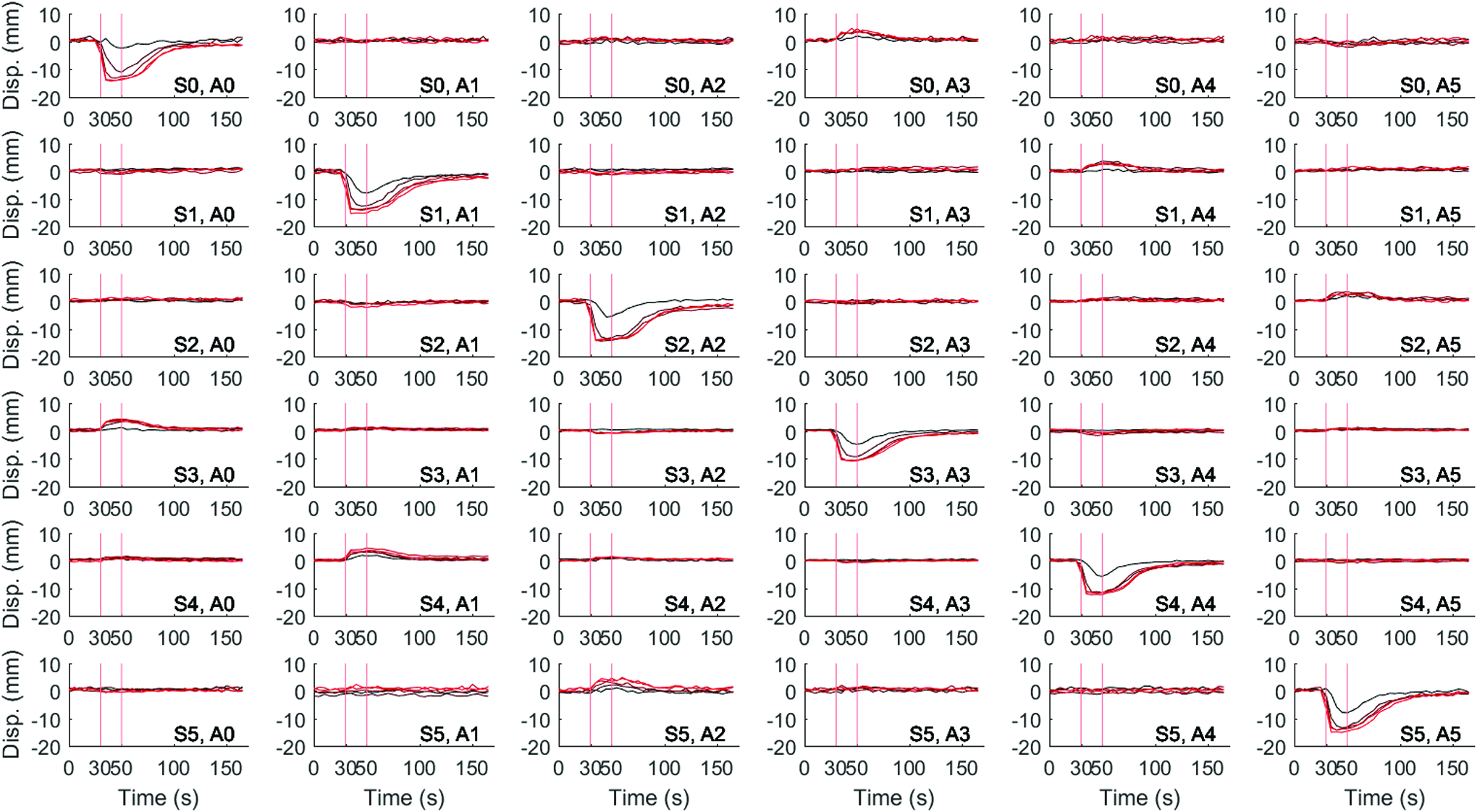
Schematic illustrations of the robot showing critical element labels. Sensors and actuators are shown as green and orange lines. (a) Shows an isometric perspective of the robot, with nodes and actuators labeled. Actuators are labeled “A0” to “A5” in orange. Orange lines represent the nominal location of the actuators. The nodes are located at the center of the attachment locations of the sensors. The attachment locations of the actuators are not specifically labeled. (b) Shows a top perspective of the robot, showing nodes, actuators, and sensors. Sensors are shown in green and labeled “S0” to “S5.” Figures 10 and 11 show side views of the robot undergoing deformations. Color images available online at www.liebertpub.com/soro
We compute the forward transformation \documentclass{aastex}\usepackage{amsbsy}\usepackage{amsfonts}\usepackage{amssymb}\usepackage{bm}\usepackage{mathrsfs}\usepackage{pifont}\usepackage{stmaryrd}\usepackage{textcomp}\usepackage{portland, xspace}\usepackage{amsmath, amsxtra}\usepackage{upgreek}\pagestyle{empty}\DeclareMathSizes{10}{9}{7}{6}\begin{document}
$${\mathcal{T}} ( { \bf{c}} )$$
\end{document} in three steps. First, we compute the location of the nodes in the top and bottom plates relative to the center of each plate. Second, we rotate the points in the top plate based on the rotation components in the state vector in Equation (1). Third, we translate the rotated points in the top plate according to the translation components in state vector in Equation (1). Starting with the points in the lower platform, which does not move, the nodal locations are:
\documentclass{aastex}\usepackage{amsbsy}\usepackage{amsfonts}\usepackage{amssymb}\usepackage{bm}\usepackage{mathrsfs}\usepackage{pifont}\usepackage{stmaryrd}\usepackage{textcomp}\usepackage{portland, xspace}\usepackage{amsmath, amsxtra}\usepackage{upgreek}\pagestyle{empty}\DeclareMathSizes{10}{9}{7}{6}\begin{document}
\begin{align*}
\begin{split}
{ { \bf { r } } _i } = &\left[ { r \cos \theta + { { ( - 1 ) } ^ { \frac { i } { 2 } { \rm { mod } } 2 + 1 } } o
\sin \theta } \right] { { \bf { e } } _1 } + \\
& \left[ { r \sin \theta + { { ( - 1 ) } ^ { \frac { i } { 2 } { \rm { mod } } 2 } } o \cos \theta } \right]
{ { \bf { e } } _2 } + \\
& 0 { \mkern 1mu } { { \bf { e } } _3 } , \\
& i \in ( 0 , 2 , 4 , \ldots , 10 ) ,
\end{split}
\tag {5}
\end{align*}
\end{document}
where r is the nominal radius of the attachment points, o is the attachment point offset, and \documentclass{aastex}\usepackage{amsbsy}\usepackage{amsfonts}\usepackage{amssymb}\usepackage{bm}\usepackage{mathrsfs}\usepackage{pifont}\usepackage{stmaryrd}\usepackage{textcomp}\usepackage{portland, xspace}\usepackage{amsmath, amsxtra}\usepackage{upgreek}\pagestyle{empty}\DeclareMathSizes{10}{9}{7}{6}\begin{document}
$$\theta$$
\end{document} is defined as:
\documentclass{aastex}\usepackage{amsbsy}\usepackage{amsfonts}\usepackage{amssymb}\usepackage{bm}\usepackage{mathrsfs}\usepackage{pifont}\usepackage{stmaryrd}\usepackage{textcomp}\usepackage{portland, xspace}\usepackage{amsmath, amsxtra}\usepackage{upgreek}\pagestyle{empty}\DeclareMathSizes{10}{9}{7}{6}\begin{document}
\begin{align*}
\theta = \left( { \left( { \frac { { i + 2 } } { 4 } { \rm { mod } } 3 } \right) \frac { { 2 \pi } } { 3 } } \right). \tag { 6 }
\end{align*}
\end{document}
Similarly, for the top plate, before the application of translation or rotation:
\documentclass{aastex}\usepackage{amsbsy}\usepackage{amsfonts}\usepackage{amssymb}\usepackage{bm}\usepackage{mathrsfs}\usepackage{pifont}\usepackage{stmaryrd}\usepackage{textcomp}\usepackage{portland, xspace}\usepackage{amsmath, amsxtra}\usepackage{upgreek}\pagestyle{empty}\DeclareMathSizes{10}{9}{7}{6}\begin{document}
\begin{align*}
\begin{split} { { \bf { r } } _i } &= \left[ { r \cos \theta + { { ( - 1 ) } ^ { \frac { { i - 1 } } { 2 } { \rm { mod } } 2 } } o \sin \theta } \right] { { \bf { e } } _1 } + \\
&\quad \left[ { r \sin \theta + { { ( - 1 ) } ^ { \frac { { i - 1 } } { 2 } { \rm { mod } } 2 + 1 } } o \cos \theta } \right] { { \bf { e } } _2 } + \\
&\quad 0 { \mkern 1mu } { { \bf { e } } _3 } , \\ &\quad i \in ( 1 , 3 , 5 , \ldots , 11 ).
\end{split}
\tag {7}
\end{align*}
\end{document}
Based on the configuration vector and the known geometry, we define a vector from the center of the lower plate to the center of the upper plate:
\documentclass{aastex}\usepackage{amsbsy}\usepackage{amsfonts}\usepackage{amssymb}\usepackage{bm}\usepackage{mathrsfs}\usepackage{pifont}\usepackage{stmaryrd}\usepackage{textcomp}\usepackage{portland, xspace}\usepackage{amsmath, amsxtra}\usepackage{upgreek}\pagestyle{empty}\DeclareMathSizes{10}{9}{7}{6}\begin{document}
\begin{align*}
{ \bf{t}} = \left\{ {{x_1}{{ \bf{e}}_1} + {x_2}{{ \bf{e}}_2} + ( {x_3} + h ) {{ \bf{e}}_3}} \right\} , \tag{8}
\end{align*}
\end{document}
where xi are the translation components of the state vector \documentclass{aastex}\usepackage{amsbsy}\usepackage{amsfonts}\usepackage{amssymb}\usepackage{bm}\usepackage{mathrsfs}\usepackage{pifont}\usepackage{stmaryrd}\usepackage{textcomp}\usepackage{portland, xspace}\usepackage{amsmath, amsxtra}\usepackage{upgreek}\pagestyle{empty}\DeclareMathSizes{10}{9}{7}{6}\begin{document}
$${ \bf{c}}$$
\end{document}, and h is the nominal separation between the two plates. To compute the location of a node on the upper plate, we use:
\documentclass{aastex}\usepackage{amsbsy}\usepackage{amsfonts}\usepackage{amssymb}\usepackage{bm}\usepackage{mathrsfs}\usepackage{pifont}\usepackage{stmaryrd}\usepackage{textcomp}\usepackage{portland, xspace}\usepackage{amsmath, amsxtra}\usepackage{upgreek}\pagestyle{empty}\DeclareMathSizes{10}{9}{7}{6}\begin{document}
\begin{align*}
{{ \bf{r}}_{i \prime }} = { \bf{q}}{{ \bf{r}}_i}{{ \bf{q}}^{ - 1}} + { \bf{t}}. \tag{9}
\end{align*}
\end{document}
where q1, q2, and q3 are the rotation components of the state vector \documentclass{aastex}\usepackage{amsbsy}\usepackage{amsfonts}\usepackage{amssymb}\usepackage{bm}\usepackage{mathrsfs}\usepackage{pifont}\usepackage{stmaryrd}\usepackage{textcomp}\usepackage{portland, xspace}\usepackage{amsmath, amsxtra}\usepackage{upgreek}\pagestyle{empty}\DeclareMathSizes{10}{9}{7}{6}\begin{document}
$${ \bf{c}}$$
\end{document}. Finally, we compute the distance between nodes:
\documentclass{aastex}\usepackage{amsbsy}\usepackage{amsfonts}\usepackage{amssymb}\usepackage{bm}\usepackage{mathrsfs}\usepackage{pifont}\usepackage{stmaryrd}\usepackage{textcomp}\usepackage{portland, xspace}\usepackage{amsmath, amsxtra}\usepackage{upgreek}\pagestyle{empty}\DeclareMathSizes{10}{9}{7}{6}\begin{document}
\begin{align*}
{l_i} = { \left\vert {{{ \bf{r}}_i} - { \bf{r}} \prime _{{i + 1}}} \right\vert _2} , i \in ( 0 , 2 , 4 , \ldots , 10 ) , \tag{11}
\end{align*}
\end{document}
where \documentclass{aastex}\usepackage{amsbsy}\usepackage{amsfonts}\usepackage{amssymb}\usepackage{bm}\usepackage{mathrsfs}\usepackage{pifont}\usepackage{stmaryrd}\usepackage{textcomp}\usepackage{portland, xspace}\usepackage{amsmath, amsxtra}\usepackage{upgreek}\pagestyle{empty}\DeclareMathSizes{10}{9}{7}{6}\begin{document}
$$\vert { \bf{v}}{ \vert _2}$$
\end{document} denotes the 2-norm of a vector and li are the elements of the internal state vector \documentclass{aastex}\usepackage{amsbsy}\usepackage{amsfonts}\usepackage{amssymb}\usepackage{bm}\usepackage{mathrsfs}\usepackage{pifont}\usepackage{stmaryrd}\usepackage{textcomp}\usepackage{portland, xspace}\usepackage{amsmath, amsxtra}\usepackage{upgreek}\pagestyle{empty}\DeclareMathSizes{10}{9}{7}{6}\begin{document}
$${ \bf{l}}$$
\end{document}. Equations (8)–(11) are the forward transformation \documentclass{aastex}\usepackage{amsbsy}\usepackage{amsfonts}\usepackage{amssymb}\usepackage{bm}\usepackage{mathrsfs}\usepackage{pifont}\usepackage{stmaryrd}\usepackage{textcomp}\usepackage{portland, xspace}\usepackage{amsmath, amsxtra}\usepackage{upgreek}\pagestyle{empty}\DeclareMathSizes{10}{9}{7}{6}\begin{document}
$$\mathcal{T}$$
\end{document}. The forward transformation is used to convert user inputs into the space used for control.
The reverse transformation is more complex, and we solve this problem by using an iterative numerical scheme. We begin by assuming a state vector (Eqn. 1), which we denote \documentclass{aastex}\usepackage{amsbsy}\usepackage{amsfonts}\usepackage{amssymb}\usepackage{bm}\usepackage{mathrsfs}\usepackage{pifont}\usepackage{stmaryrd}\usepackage{textcomp}\usepackage{portland, xspace}\usepackage{amsmath, amsxtra}\usepackage{upgreek}\pagestyle{empty}\DeclareMathSizes{10}{9}{7}{6}\begin{document}
$${{ \bf{c}}_{est}}$$
\end{document}. We assume a zero-configuration vector, although using the previous solution as a starting point improves the performance of the algorithm at the cost of increased memory storage. Based on this initial estimate, and using the forward transformation described earlier, we compute a set of estimated sensor lengths:
\documentclass{aastex}\usepackage{amsbsy}\usepackage{amsfonts}\usepackage{amssymb}\usepackage{bm}\usepackage{mathrsfs}\usepackage{pifont}\usepackage{stmaryrd}\usepackage{textcomp}\usepackage{portland, xspace}\usepackage{amsmath, amsxtra}\usepackage{upgreek}\pagestyle{empty}\DeclareMathSizes{10}{9}{7}{6}\begin{document}
\begin{align*}
{{ \bf{l}}_{est}} = \mathcal{T} ( {{ \bf{c}}_{est}} ). \tag{12}
\end{align*}
\end{document}
Next, we compute the error in the sensor lengths:
\documentclass{aastex}\usepackage{amsbsy}\usepackage{amsfonts}\usepackage{amssymb}\usepackage{bm}\usepackage{mathrsfs}\usepackage{pifont}\usepackage{stmaryrd}\usepackage{textcomp}\usepackage{portland, xspace}\usepackage{amsmath, amsxtra}\usepackage{upgreek}\pagestyle{empty}\DeclareMathSizes{10}{9}{7}{6}\begin{document}
\begin{align*}
{ \bf{e}} = {{ \bf{l}}_{mes}} - {{ \bf{l}}_{est}} , \tag{13}
\end{align*}
\end{document}
where \documentclass{aastex}\usepackage{amsbsy}\usepackage{amsfonts}\usepackage{amssymb}\usepackage{bm}\usepackage{mathrsfs}\usepackage{pifont}\usepackage{stmaryrd}\usepackage{textcomp}\usepackage{portland, xspace}\usepackage{amsmath, amsxtra}\usepackage{upgreek}\pagestyle{empty}\DeclareMathSizes{10}{9}{7}{6}\begin{document}
$${{ \bf{l}}_{mes}}$$
\end{document} is the measured internal state vector provided from the sensor outputs. We use the Newton-Raphson algorithm to minimize the error in lengths. Since the system is fully defined, we can achieve a solution with arbitrary numerical precision, although the accuracy of the solution is limited by the accuracy of the sensor observations. To compute the required Jacobian, we perturb the configuration vector and determine the change in error due to the perturbation. In the case of the translation components, this is trivial. In the case of the rotations, we apply perturbations of \documentclass{aastex}\usepackage{amsbsy}\usepackage{amsfonts}\usepackage{amssymb}\usepackage{bm}\usepackage{mathrsfs}\usepackage{pifont}\usepackage{stmaryrd}\usepackage{textcomp}\usepackage{portland, xspace}\usepackage{amsmath, amsxtra}\usepackage{upgreek}\pagestyle{empty}\DeclareMathSizes{10}{9}{7}{6}\begin{document}
$$0.001rad$$
\end{document} in the local yaw, pitch, and roll directions in the local coordinate system of the moving platform based on the current estimate. We denote these perturbations as \documentclass{aastex}\usepackage{amsbsy}\usepackage{amsfonts}\usepackage{amssymb}\usepackage{bm}\usepackage{mathrsfs}\usepackage{pifont}\usepackage{stmaryrd}\usepackage{textcomp}\usepackage{portland, xspace}\usepackage{amsmath, amsxtra}\usepackage{upgreek}\pagestyle{empty}\DeclareMathSizes{10}{9}{7}{6}\begin{document}
$$\rho$$
\end{document}. Formally, in quaternion notation in the local coordinate system attached to the moving platform, they are:
\documentclass{aastex}\usepackage{amsbsy}\usepackage{amsfonts}\usepackage{amssymb}\usepackage{bm}\usepackage{mathrsfs}\usepackage{pifont}\usepackage{stmaryrd}\usepackage{textcomp}\usepackage{portland, xspace}\usepackage{amsmath, amsxtra}\usepackage{upgreek}\pagestyle{empty}\DeclareMathSizes{10}{9}{7}{6}\begin{document}
\begin{align*}
{ \rho _1} = \left\{ {0.001 , 1 , 0 , 0} \right\} , \tag{14{\rm a}}
\end{align*}
\end{document}\documentclass{aastex}\usepackage{amsbsy}\usepackage{amsfonts}\usepackage{amssymb}\usepackage{bm}\usepackage{mathrsfs}\usepackage{pifont}\usepackage{stmaryrd}\usepackage{textcomp}\usepackage{portland, xspace}\usepackage{amsmath, amsxtra}\usepackage{upgreek}\pagestyle{empty}\DeclareMathSizes{10}{9}{7}{6}\begin{document}
\begin{align*}
{ \rho _2} = \left\{ {0.001 , 0 , 1 , 0} \right\} , \tag{14{\rm b}}
\end{align*}
\end{document}\documentclass{aastex}\usepackage{amsbsy}\usepackage{amsfonts}\usepackage{amssymb}\usepackage{bm}\usepackage{mathrsfs}\usepackage{pifont}\usepackage{stmaryrd}\usepackage{textcomp}\usepackage{portland, xspace}\usepackage{amsmath, amsxtra}\usepackage{upgreek}\pagestyle{empty}\DeclareMathSizes{10}{9}{7}{6}\begin{document}
\begin{align*}
{ \rho _3} = \left\{ {0.001 , 0 , 0 , 1} \right\} . \tag{14{\rm c}}
\end{align*}
\end{document}
where the error terms ei are the components of the error vector defined in Equation (13). We use lower-upper (LU) decomposition to solve the system of equations:
\documentclass{aastex}\usepackage{amsbsy}\usepackage{amsfonts}\usepackage{amssymb}\usepackage{bm}\usepackage{mathrsfs}\usepackage{pifont}\usepackage{stmaryrd}\usepackage{textcomp}\usepackage{portland, xspace}\usepackage{amsmath, amsxtra}\usepackage{upgreek}\pagestyle{empty}\DeclareMathSizes{10}{9}{7}{6}\begin{document}
\begin{align*}
{ \bf{J}} \left( {{ \bf{c}}_{est}^{ ( n + 1 ) } - { \bf{c}}_{est}^{ ( n ) }} \right) = - \epsilon , \tag{16}
\end{align*}
\end{document}
where the \documentclass{aastex}\usepackage{amsbsy}\usepackage{amsfonts}\usepackage{amssymb}\usepackage{bm}\usepackage{mathrsfs}\usepackage{pifont}\usepackage{stmaryrd}\usepackage{textcomp}\usepackage{portland, xspace}\usepackage{amsmath, amsxtra}\usepackage{upgreek}\pagestyle{empty}\DeclareMathSizes{10}{9}{7}{6}\begin{document}
$$( n + 1 )$$
\end{document}and \documentclass{aastex}\usepackage{amsbsy}\usepackage{amsfonts}\usepackage{amssymb}\usepackage{bm}\usepackage{mathrsfs}\usepackage{pifont}\usepackage{stmaryrd}\usepackage{textcomp}\usepackage{portland, xspace}\usepackage{amsmath, amsxtra}\usepackage{upgreek}\pagestyle{empty}\DeclareMathSizes{10}{9}{7}{6}\begin{document}
$$( n )$$
\end{document}superscripts denote the iteration number.
The required step between \documentclass{aastex}\usepackage{amsbsy}\usepackage{amsfonts}\usepackage{amssymb}\usepackage{bm}\usepackage{mathrsfs}\usepackage{pifont}\usepackage{stmaryrd}\usepackage{textcomp}\usepackage{portland, xspace}\usepackage{amsmath, amsxtra}\usepackage{upgreek}\pagestyle{empty}\DeclareMathSizes{10}{9}{7}{6}\begin{document}
$${ \bf{c}}_{est}^{ ( n + 1 ) }$$
\end{document} and \documentclass{aastex}\usepackage{amsbsy}\usepackage{amsfonts}\usepackage{amssymb}\usepackage{bm}\usepackage{mathrsfs}\usepackage{pifont}\usepackage{stmaryrd}\usepackage{textcomp}\usepackage{portland, xspace}\usepackage{amsmath, amsxtra}\usepackage{upgreek}\pagestyle{empty}\DeclareMathSizes{10}{9}{7}{6}\begin{document}
$${ \bf{c}}_{est}^{ ( n ) }$$
\end{document} for the translation components \documentclass{aastex}\usepackage{amsbsy}\usepackage{amsfonts}\usepackage{amssymb}\usepackage{bm}\usepackage{mathrsfs}\usepackage{pifont}\usepackage{stmaryrd}\usepackage{textcomp}\usepackage{portland, xspace}\usepackage{amsmath, amsxtra}\usepackage{upgreek}\pagestyle{empty}\DeclareMathSizes{10}{9}{7}{6}\begin{document}
$${x_1} , {x_2} , {x_3}$$
\end{document} is trivial to apply.
However, rotations do not exhibit superposition, and so they must be added sequentially. We apply the largest rotation step first (as measured by the magnitude of the rotation angle), followed by the second and third largest. This approach minimizes the error between the step determined by using the iteration scheme and the actual step applied. Ultimately, as the solution converges and the step size decreases, this effect becomes negligible.
We used a convergence criterion of 1 × 10⁻⁶ cm based on the 2-norm of the error vector \documentclass{aastex}\usepackage{amsbsy}\usepackage{amsfonts}\usepackage{amssymb}\usepackage{bm}\usepackage{mathrsfs}\usepackage{pifont}\usepackage{stmaryrd}\usepackage{textcomp}\usepackage{portland, xspace}\usepackage{amsmath, amsxtra}\usepackage{upgreek}\pagestyle{empty}\DeclareMathSizes{10}{9}{7}{6}\begin{document}
$$\epsilon$$
\end{document}. Convergence occurred in less than five iterations in most cases. We implemented this entire algorithm in Cython, which is a language based on Python with the static variable typing of C. This was imported into our overall interface and control software, which was written in regular Python. Running on a 2.60 GHz 64-bit computer with Ubuntu Linux, convergence required less than 1 ms, which was sufficiently brief so that the numeric inversion could be integrated into a control loop.
Experimental
The robot was fabricated in three steps. The capacitive sensors and SMA actuators were fabricated in two separate parallel processes, then integrated together into a complete system with passive elements. The capacitive sensor fabrication process is novel and presented in more detail, whereas the SMA programming procedure is well known and only summarized.
Capacitive Sensor Fabrication
Capacitive sensors were fabricated from three-layer structures of conductive composite elastomer electrodes coating a non-conductive dielectric layer. All of the layers were based on Dragon Skin 10 elastomer (Smooth-On, Inc.). The conductive composite material was made from 10 wt% expanded intercalated graphite (EIG). The EIG was made by soaking graphite flakes (Sigma-Aldrich) in a \documentclass{aastex}\usepackage{amsbsy}\usepackage{amsfonts}\usepackage{amssymb}\usepackage{bm}\usepackage{mathrsfs}\usepackage{pifont}\usepackage{stmaryrd}\usepackage{textcomp}\usepackage{portland, xspace}\usepackage{amsmath, amsxtra}\usepackage{upgreek}\pagestyle{empty}\DeclareMathSizes{10}{9}{7}{6}\begin{document}
$$4:1$$
\end{document} nitric acid:sulfuric acid solution, followed by roasting at 800°C for 5 min. This soaking and roasting process caused the graphene plates within the graphite to partially pull apart (“exfoliate”), resulting in a loose connection between plates. We then soaked the expanded material in cyclohexane and sonicated by using a tip sonicator (Q700 with 1/4″ tip, Qsonica) for 1 h at an amplitude of 36 μm to further separate the plates. Finally, we dried the resulting slurry to a concentration between 3 wt% and 5 wt%. To make the composite material, we combined pre-mixed Dragon Skin 10 with EIG slurry and additional cyclohexane to achieve a concentration of 3.00 wt% of graphite in the wet material, and 10.0 wt% in the finished composite.
Three-layer blank substrates were fabricated by using a rod-coating process, which we have previously described.36 A 1/4″-10 Acme threaded rod (McMaster-Carr) was used to apply a uniform layer of liquid composite elastomer to a polyethylene terephthalate (PET) substrate. Liquid conductive elastomer was poured onto the PET film, then scraped across the surface by using the threaded rod. The liquid elastomer owed through the threads in the rod, forming a uniform film. This electrode layer was allowed to cure, which generally took between 4 and 8 h due to the evaporation of cyclohexane. Once cured, we applied a layer of normal Dragon Skin 10 elastomer without the inclusion of EIG as a dielectric. We poured the liquid dielectric layer directly onto the cured electrode layer and used an identical rod-coating procedure to create a uniform film. Immediately after casting the film, we applied elastomer-impregnated muslin fabric to the curing film at the ends of the sensor elements as a reinforcement tab. The dielectric layer, with fabric tabs, was allowed to cure for ∼45 min until it achieved a “tacky” consistency. At this point, we folded the sheet in half and bonded the tacky dielectric layer to itself. This resulted in a six-layer structure: PET—conductive composite—dielectric— dielectric—conductive composite—PET. We allowed this layered structure to sit at room temperature for at least 4 h to complete curing. Using the fabric tabs as alignment guides, we cut the final sensor shapes from the completed elastomer substrate by using a Universal Laser Systems VLS 2.30 patterning system fitted with a 30 W \documentclass{aastex}\usepackage{amsbsy}\usepackage{amsfonts}\usepackage{amssymb}\usepackage{bm}\usepackage{mathrsfs}\usepackage{pifont}\usepackage{stmaryrd}\usepackage{textcomp}\usepackage{portland, xspace}\usepackage{amsmath, amsxtra}\usepackage{upgreek}\pagestyle{empty}\DeclareMathSizes{10}{9}{7}{6}\begin{document}
$${ \rm{C}}{{ \rm{O}}_{ \rm{2}}}$$
\end{document} laser module. The backing PET layer was removed from the completed sensors, and soot from the laser patterning process was cleaned by using a soap solution (Liquinox, Alconox).
Once cut from the elastomer substrate, the deformable component of the capacitive sensor was attached to polystyrene attachment tabs, interface electrodes, and electronics. To begin this attachment, we sewed two laser-cut polystyrene (PS) tabs to the front and back of one end of the sensor by using cotton thread. We cut matching holes in the PS and sensor structure to facilitate sewing. On one side of the sensor, we attached only the PS, whereas on the other side we inserted Pyralux (Adafruit) leads to provide electrical contact to the two electrodes on the sensor. We soldered these leads to a printed circuit board containing the electronics, then finished by sewing the circuit board to the PS tabs.
Capacitive Sensor Functionality
The capacitive sensor is shaped like a “dog bone” material testing sample, and it consists of an inner deformable region with two nondeformable regions at the ends. These nondeformable regions are made rigid through the inclusion of fabric into the dielectric material and are included to provide a mechanical attachment. In addition to the capacitance of these regions of the sensor, there is also a parasitic contribution from the electrical interface and the signal conditioning electronics. In operation, all of these sources combine into a baseline capacitance. As we show in our later discussion on calibration, the baseline capacitance can be removed, with the result being that only the change in capacitance is related to strain. Since the body of the sensor is a parallel-plate capacitor, the capacitance of the active region is related to the geometry by:
\documentclass{aastex}\usepackage{amsbsy}\usepackage{amsfonts}\usepackage{amssymb}\usepackage{bm}\usepackage{mathrsfs}\usepackage{pifont}\usepackage{stmaryrd}\usepackage{textcomp}\usepackage{portland, xspace}\usepackage{amsmath, amsxtra}\usepackage{upgreek}\pagestyle{empty}\DeclareMathSizes{10}{9}{7}{6}\begin{document}
\begin{align*}
{ C_ { Active } } = { \epsilon _0 } { \epsilon _r } \frac { a } { t } = { \epsilon _0 } { \epsilon _r } \frac { { wl } } { t } , \tag { 17 }
\end{align*}
\end{document}
where \documentclass{aastex}\usepackage{amsbsy}\usepackage{amsfonts}\usepackage{amssymb}\usepackage{bm}\usepackage{mathrsfs}\usepackage{pifont}\usepackage{stmaryrd}\usepackage{textcomp}\usepackage{portland, xspace}\usepackage{amsmath, amsxtra}\usepackage{upgreek}\pagestyle{empty}\DeclareMathSizes{10}{9}{7}{6}\begin{document}
$${ \epsilon _0}$$
\end{document} is the permittivity of free space, \documentclass{aastex}\usepackage{amsbsy}\usepackage{amsfonts}\usepackage{amssymb}\usepackage{bm}\usepackage{mathrsfs}\usepackage{pifont}\usepackage{stmaryrd}\usepackage{textcomp}\usepackage{portland, xspace}\usepackage{amsmath, amsxtra}\usepackage{upgreek}\pagestyle{empty}\DeclareMathSizes{10}{9}{7}{6}\begin{document}
$${ \epsilon _r}$$
\end{document} is the relative permittivity of the dielectric material, a is the planform area of the device (as opposed to the cross-section area), t is the thickness of the sensor, w is the width, and l is the length. Assuming the material is incompressible and homogeneous, and by introducing a linear strain \documentclass{aastex}\usepackage{amsbsy}\usepackage{amsfonts}\usepackage{amssymb}\usepackage{bm}\usepackage{mathrsfs}\usepackage{pifont}\usepackage{stmaryrd}\usepackage{textcomp}\usepackage{portland, xspace}\usepackage{amsmath, amsxtra}\usepackage{upgreek}\pagestyle{empty}\DeclareMathSizes{10}{9}{7}{6}\begin{document}
$$\varepsilon$$
\end{document} such that \documentclass{aastex}\usepackage{amsbsy}\usepackage{amsfonts}\usepackage{amssymb}\usepackage{bm}\usepackage{mathrsfs}\usepackage{pifont}\usepackage{stmaryrd}\usepackage{textcomp}\usepackage{portland, xspace}\usepackage{amsmath, amsxtra}\usepackage{upgreek}\pagestyle{empty}\DeclareMathSizes{10}{9}{7}{6}\begin{document}
$$l = {l_0} ( 1 + \varepsilon )$$
\end{document} where \documentclass{aastex}\usepackage{amsbsy}\usepackage{amsfonts}\usepackage{amssymb}\usepackage{bm}\usepackage{mathrsfs}\usepackage{pifont}\usepackage{stmaryrd}\usepackage{textcomp}\usepackage{portland, xspace}\usepackage{amsmath, amsxtra}\usepackage{upgreek}\pagestyle{empty}\DeclareMathSizes{10}{9}{7}{6}\begin{document}
$${{ \rm{l}}_0}$$
\end{document} is the initial length, the deformed width and thickness are \documentclass{aastex}\usepackage{amsbsy}\usepackage{amsfonts}\usepackage{amssymb}\usepackage{bm}\usepackage{mathrsfs}\usepackage{pifont}\usepackage{stmaryrd}\usepackage{textcomp}\usepackage{portland, xspace}\usepackage{amsmath, amsxtra}\usepackage{upgreek}\pagestyle{empty}\DeclareMathSizes{10}{9}{7}{6}\begin{document}
$${w_0} = { ( 1 + \varepsilon ) ^{ - 0.5}}$$
\end{document} and \documentclass{aastex}\usepackage{amsbsy}\usepackage{amsfonts}\usepackage{amssymb}\usepackage{bm}\usepackage{mathrsfs}\usepackage{pifont}\usepackage{stmaryrd}\usepackage{textcomp}\usepackage{portland, xspace}\usepackage{amsmath, amsxtra}\usepackage{upgreek}\pagestyle{empty}\DeclareMathSizes{10}{9}{7}{6}\begin{document}
$$t = {t_0}{ ( 1 + \varepsilon ) ^{ - 0.5}}$$
\end{document}. Substituting the deformed geometry, we have the capacitance as a function of strain:
\documentclass{aastex}\usepackage{amsbsy}\usepackage{amsfonts}\usepackage{amssymb}\usepackage{bm}\usepackage{mathrsfs}\usepackage{pifont}\usepackage{stmaryrd}\usepackage{textcomp}\usepackage{portland, xspace}\usepackage{amsmath, amsxtra}\usepackage{upgreek}\pagestyle{empty}\DeclareMathSizes{10}{9}{7}{6}\begin{document}
\begin{align*}
{ C_ { Active } } = { \epsilon _0 } { \epsilon _r } { \frac { { w_0 } { l_0 } } { { t_0 } } } \left( { 1 + \varepsilon } \right). \tag { 18 }
\end{align*}
\end{document}
To measure the capacitance, we utilize a fixed-frequency oscillator. The critical timing events of the oscillation are shown in Figure 3a, and the charge and discharge circuit is shown in Figure 3b. The concept is to control the duty cycle of a fixed frequency square wave by using the capacitance of the sensor, then filter that signal through a low-pass filter to recover the average output. The governing equation for the voltage across the capacitor while charging is:
\documentclass{aastex}\usepackage{amsbsy}\usepackage{amsfonts}\usepackage{amssymb}\usepackage{bm}\usepackage{mathrsfs}\usepackage{pifont}\usepackage{stmaryrd}\usepackage{textcomp}\usepackage{portland, xspace}\usepackage{amsmath, amsxtra}\usepackage{upgreek}\pagestyle{empty}\DeclareMathSizes{10}{9}{7}{6}\begin{document}
\begin{align*}
C { \frac { d { V_c } } { dt } } + \frac { 1 } { { { R_D } } } { V_c } + \frac { 1 } { { { R_C } } } { V_c } = \frac { 1 } { { { R_C } } } { V_ { In } } ,
\end{align*}
\end{document}
where C is the capacitance of the sensor (which is the sum of both parasitic and active components), Vc is the voltage across the sensor, RD is the fixed discharge resistor, RC is the fixed charge resistor, and \documentclass{aastex}\usepackage{amsbsy}\usepackage{amsfonts}\usepackage{amssymb}\usepackage{bm}\usepackage{mathrsfs}\usepackage{pifont}\usepackage{stmaryrd}\usepackage{textcomp}\usepackage{portland, xspace}\usepackage{amsmath, amsxtra}\usepackage{upgreek}\pagestyle{empty}\DeclareMathSizes{10}{9}{7}{6}\begin{document}
$${V_{In}}$$
\end{document} is the input voltage to the RC network. In the time domain, the solution is:
\documentclass{aastex}\usepackage{amsbsy}\usepackage{amsfonts}\usepackage{amssymb}\usepackage{bm}\usepackage{mathrsfs}\usepackage{pifont}\usepackage{stmaryrd}\usepackage{textcomp}\usepackage{portland, xspace}\usepackage{amsmath, amsxtra}\usepackage{upgreek}\pagestyle{empty}\DeclareMathSizes{10}{9}{7}{6}\begin{document}
\begin{align*}
{ V_c } ( t ) = { \frac { { R_D } } { { R_C } + { R_D } } } \left( { 1 - { e^ { - \left( { { \frac { { R_C } + { R_D } } { { R_C } { R_D } C } } } \right) t } } } \right) { V_ { In } } . \tag { 19 }
\end{align*}
\end{document}
Using a similar process, in the discharging case, the voltage across the sensor is:
\documentclass{aastex}\usepackage{amsbsy}\usepackage{amsfonts}\usepackage{amssymb}\usepackage{bm}\usepackage{mathrsfs}\usepackage{pifont}\usepackage{stmaryrd}\usepackage{textcomp}\usepackage{portland, xspace}\usepackage{amsmath, amsxtra}\usepackage{upgreek}\pagestyle{empty}\DeclareMathSizes{10}{9}{7}{6}\begin{document}
\begin{align*}
{ V_c } ( t ) = { e^ { - \left( { \frac { 1 } { { { R_D } C } } } \right) t } } { V_h } , \tag { 20 }
\end{align*}
\end{document}
where Vh is the initial voltage across the sensor, which we call the “high threshold voltage.” In operation, we charge the capacitor from \documentclass{aastex}\usepackage{amsbsy}\usepackage{amsfonts}\usepackage{amssymb}\usepackage{bm}\usepackage{mathrsfs}\usepackage{pifont}\usepackage{stmaryrd}\usepackage{textcomp}\usepackage{portland, xspace}\usepackage{amsmath, amsxtra}\usepackage{upgreek}\pagestyle{empty}\DeclareMathSizes{10}{9}{7}{6}\begin{document}
$$0V$$
\end{document} to Vh, then discharge back to a lower threshold voltage Vl. During both the charge and discharge operations, we drive a status pin high, which generates the variable pulse width signal that is fed into the filter. Theoretically, we can set \documentclass{aastex}\usepackage{amsbsy}\usepackage{amsfonts}\usepackage{amssymb}\usepackage{bm}\usepackage{mathrsfs}\usepackage{pifont}\usepackage{stmaryrd}\usepackage{textcomp}\usepackage{portland, xspace}\usepackage{amsmath, amsxtra}\usepackage{upgreek}\pagestyle{empty}\DeclareMathSizes{10}{9}{7}{6}\begin{document}
$$ { V_h } \in ( 0V , { \frac { { R_D } } { { R_C } + { R_D } } } { V_ { In } } )$$
\end{document} and \documentclass{aastex}\usepackage{amsbsy}\usepackage{amsfonts}\usepackage{amssymb}\usepackage{bm}\usepackage{mathrsfs}\usepackage{pifont}\usepackage{stmaryrd}\usepackage{textcomp}\usepackage{portland, xspace}\usepackage{amsmath, amsxtra}\usepackage{upgreek}\pagestyle{empty}\DeclareMathSizes{10}{9}{7}{6}\begin{document}
$${V_l} \in ( 0V , {V_h} )$$
\end{document}. We will discuss the practical issues associated with these values later. From Equation (19), the time required to charge the sensor is:
\documentclass{aastex}\usepackage{amsbsy}\usepackage{amsfonts}\usepackage{amssymb}\usepackage{bm}\usepackage{mathrsfs}\usepackage{pifont}\usepackage{stmaryrd}\usepackage{textcomp}\usepackage{portland, xspace}\usepackage{amsmath, amsxtra}\usepackage{upgreek}\pagestyle{empty}\DeclareMathSizes{10}{9}{7}{6}\begin{document}
\begin{align*}
{ t_h } = - { \frac { { R_C } { R_D } C } { { R_C } + { R_D } } } { \rm { ln } } \left( { - { \frac { { V_h } } { { V_ { In } } } } { \frac { { R_C } + { R_D } } { { R_D } } } + 1 } \right) ,
\end{align*}
\end{document}
where th denotes the time to charge to Vh. Likewise, from Equation (20), the time required to discharge from Vh to Vl is:
\documentclass{aastex}\usepackage{amsbsy}\usepackage{amsfonts}\usepackage{amssymb}\usepackage{bm}\usepackage{mathrsfs}\usepackage{pifont}\usepackage{stmaryrd}\usepackage{textcomp}\usepackage{portland, xspace}\usepackage{amsmath, amsxtra}\usepackage{upgreek}\pagestyle{empty}\DeclareMathSizes{10}{9}{7}{6}\begin{document}
\begin{align*}
{ t_l } = - { R_D } C { \rm { ln } } \left( { { \frac { { V_l } } { { V_h } } } } \right).
\end{align*}
\end{document}
Adding these times together into a single expression:
\documentclass{aastex}\usepackage{amsbsy}\usepackage{amsfonts}\usepackage{amssymb}\usepackage{bm}\usepackage{mathrsfs}\usepackage{pifont}\usepackage{stmaryrd}\usepackage{textcomp}\usepackage{portland, xspace}\usepackage{amsmath, amsxtra}\usepackage{upgreek}\pagestyle{empty}\DeclareMathSizes{10}{9}{7}{6}\begin{document}
\begin{align*}
{t_{Tot}} = {t_h} + {t_l} = \alpha C , \tag{21}
\end{align*}
\end{document}
in which all the terms are constants. Substituting in Equation (18), we obtain a relationship between the cycle time and strain:
\documentclass{aastex}\usepackage{amsbsy}\usepackage{amsfonts}\usepackage{amssymb}\usepackage{bm}\usepackage{mathrsfs}\usepackage{pifont}\usepackage{stmaryrd}\usepackage{textcomp}\usepackage{portland, xspace}\usepackage{amsmath, amsxtra}\usepackage{upgreek}\pagestyle{empty}\DeclareMathSizes{10}{9}{7}{6}\begin{document}
\begin{align*}
{ t_ { Tot } } = \alpha \left( { { \epsilon _0 } { \epsilon _r } { \frac { { w_0 } { l_0 } } { { t_0 } } } \left( { 1 + \varepsilon } \right) + { C_ { Parasitic } } } \right) ,
\end{align*}
\end{document}
where \documentclass{aastex}\usepackage{amsbsy}\usepackage{amsfonts}\usepackage{amssymb}\usepackage{bm}\usepackage{mathrsfs}\usepackage{pifont}\usepackage{stmaryrd}\usepackage{textcomp}\usepackage{portland, xspace}\usepackage{amsmath, amsxtra}\usepackage{upgreek}\pagestyle{empty}\DeclareMathSizes{10}{9}{7}{6}\begin{document}
$${C_{Parasitic}}$$
\end{document} is added to account for the capacitance of the inactive (nondeformable) part of the sensor and the signal conditioning board. The timing is ultimately simplified to:
\documentclass{aastex}\usepackage{amsbsy}\usepackage{amsfonts}\usepackage{amssymb}\usepackage{bm}\usepackage{mathrsfs}\usepackage{pifont}\usepackage{stmaryrd}\usepackage{textcomp}\usepackage{portland, xspace}\usepackage{amsmath, amsxtra}\usepackage{upgreek}\pagestyle{empty}\DeclareMathSizes{10}{9}{7}{6}\begin{document}
\begin{align*}
{t_{Tot}} = { \beta _1} \varepsilon + { \beta _0} , \tag{22}
\end{align*}
\end{document}
(a) Voltage across capacitive sensor as a function of time. Solid black line represents voltage history across the sensor for a nominal strain state. The dashed black line represents the voltage history for a higher strain state. Timing events are labeled under the horizontal axis. Threshold voltages are labeled on the vertical axis. The meaning of these values is described in the text. (b) Capacitive sensor charging and discharging circuit.
To understand the effect of the low-pass filter on the pulse train, we consider the Fourier series expansion of the sensor charge signal. By setting the cutoff frequency of the filter below (ideally at least two decades below) the fundamental frequency of the sensor charging frequency, we can neglect the harmonic terms, and are left with only the direct current (DC) contribution:
\documentclass{aastex}\usepackage{amsbsy}\usepackage{amsfonts}\usepackage{amssymb}\usepackage{bm}\usepackage{mathrsfs}\usepackage{pifont}\usepackage{stmaryrd}\usepackage{textcomp}\usepackage{portland, xspace}\usepackage{amsmath, amsxtra}\usepackage{upgreek}\pagestyle{empty}\DeclareMathSizes{10}{9}{7}{6}\begin{document}
\begin{align*}
{ V_ { DC } } = \frac { 1 } { T } \int_0^T { { V_ { Sig } } ( \tau ) d \tau } ,
\end{align*}
\end{document}
where T is the fixed period of the charging process, and VSig is a charging status indicator. VSig is high whenever the sensor is charging or discharging and low otherwise; the output voltage becomes:
\documentclass{aastex}\usepackage{amsbsy}\usepackage{amsfonts}\usepackage{amssymb}\usepackage{bm}\usepackage{mathrsfs}\usepackage{pifont}\usepackage{stmaryrd}\usepackage{textcomp}\usepackage{portland, xspace}\usepackage{amsmath, amsxtra}\usepackage{upgreek}\pagestyle{empty}\DeclareMathSizes{10}{9}{7}{6}\begin{document}
\begin{align*}
{ V_ { DC } } = \frac { 1 } { T } \left( { \int_0^ { { t_ { Tot } } } { { V_ { In } } ( \tau ) d \tau } + \int_ { { t_ { Tot } } } ^t { 0 ( \tau ) d \tau } } \right).
\end{align*}
\end{document}
Substituting in for the total charge cycle time \documentclass{aastex}\usepackage{amsbsy}\usepackage{amsfonts}\usepackage{amssymb}\usepackage{bm}\usepackage{mathrsfs}\usepackage{pifont}\usepackage{stmaryrd}\usepackage{textcomp}\usepackage{portland, xspace}\usepackage{amsmath, amsxtra}\usepackage{upgreek}\pagestyle{empty}\DeclareMathSizes{10}{9}{7}{6}\begin{document}
$${t_{Tot}}$$
\end{document} from Equation (22):
\documentclass{aastex}\usepackage{amsbsy}\usepackage{amsfonts}\usepackage{amssymb}\usepackage{bm}\usepackage{mathrsfs}\usepackage{pifont}\usepackage{stmaryrd}\usepackage{textcomp}\usepackage{portland, xspace}\usepackage{amsmath, amsxtra}\usepackage{upgreek}\pagestyle{empty}\DeclareMathSizes{10}{9}{7}{6}\begin{document}
\begin{align*}
{ V_ { DC } } = \frac { { { \beta _1 } \varepsilon + { \beta _0 } } } { T } . \tag { 24 }
\end{align*}
\end{document}
The conclusion is that the output voltage is a linear function of strain. The coefficients \documentclass{aastex}\usepackage{amsbsy}\usepackage{amsfonts}\usepackage{amssymb}\usepackage{bm}\usepackage{mathrsfs}\usepackage{pifont}\usepackage{stmaryrd}\usepackage{textcomp}\usepackage{portland, xspace}\usepackage{amsmath, amsxtra}\usepackage{upgreek}\pagestyle{empty}\DeclareMathSizes{10}{9}{7}{6}\begin{document}
$${ \beta _1}$$
\end{document} and \documentclass{aastex}\usepackage{amsbsy}\usepackage{amsfonts}\usepackage{amssymb}\usepackage{bm}\usepackage{mathrsfs}\usepackage{pifont}\usepackage{stmaryrd}\usepackage{textcomp}\usepackage{portland, xspace}\usepackage{amsmath, amsxtra}\usepackage{upgreek}\pagestyle{empty}\DeclareMathSizes{10}{9}{7}{6}\begin{document}
$${ \beta _0}$$
\end{document} contain many terms, some of which are difficult to measure individually in practice, such as \documentclass{aastex}\usepackage{amsbsy}\usepackage{amsfonts}\usepackage{amssymb}\usepackage{bm}\usepackage{mathrsfs}\usepackage{pifont}\usepackage{stmaryrd}\usepackage{textcomp}\usepackage{portland, xspace}\usepackage{amsmath, amsxtra}\usepackage{upgreek}\pagestyle{empty}\DeclareMathSizes{10}{9}{7}{6}\begin{document}
$${C_{Parasitic}}$$
\end{document}. However, this is easily overcome since the terms appear as groups that are easy to measure collectively, such as \documentclass{aastex}\usepackage{amsbsy}\usepackage{amsfonts}\usepackage{amssymb}\usepackage{bm}\usepackage{mathrsfs}\usepackage{pifont}\usepackage{stmaryrd}\usepackage{textcomp}\usepackage{portland, xspace}\usepackage{amsmath, amsxtra}\usepackage{upgreek}\pagestyle{empty}\DeclareMathSizes{10}{9}{7}{6}\begin{document}
$${ \beta _1}$$
\end{document} and \documentclass{aastex}\usepackage{amsbsy}\usepackage{amsfonts}\usepackage{amssymb}\usepackage{bm}\usepackage{mathrsfs}\usepackage{pifont}\usepackage{stmaryrd}\usepackage{textcomp}\usepackage{portland, xspace}\usepackage{amsmath, amsxtra}\usepackage{upgreek}\pagestyle{empty}\DeclareMathSizes{10}{9}{7}{6}\begin{document}
$${ \beta _0}$$
\end{document}. As we discuss later in our Results section, using a regression analysis with experimental data yields a very accurate relationship between strain and output voltage.
In designing a capacitive sensor signal conditioning system for a given application, there are a few issues to consider. First, the charge resistance RC should be lower than the discharge resistance RD. This has the effect of increasing the voltage to which the sensor can be charged, which, in turn, has the effect of reducing noise. Second, the cycle period T needs to be long enough to allow for complete charging and discharging of the sensor, but it should be as short as possible to maximize sensitivity. Third, the high threshold voltage Vh to which the sensor is charged should be balanced between maximizing sensitivity and minimizing charge time. In practice, we have found that \documentclass{aastex}\usepackage{amsbsy}\usepackage{amsfonts}\usepackage{amssymb}\usepackage{bm}\usepackage{mathrsfs}\usepackage{pifont}\usepackage{stmaryrd}\usepackage{textcomp}\usepackage{portland, xspace}\usepackage{amsmath, amsxtra}\usepackage{upgreek}\pagestyle{empty}\DeclareMathSizes{10}{9}{7}{6}\begin{document}
$$ { V_h } \approx \frac { 1 } { 2 } { V_ { In } } $$
\end{document} works for most cases. Finally, \documentclass{aastex}\usepackage{amsbsy}\usepackage{amsfonts}\usepackage{amssymb}\usepackage{bm}\usepackage{mathrsfs}\usepackage{pifont}\usepackage{stmaryrd}\usepackage{textcomp}\usepackage{portland, xspace}\usepackage{amsmath, amsxtra}\usepackage{upgreek}\pagestyle{empty}\DeclareMathSizes{10}{9}{7}{6}\begin{document}
$${{ \rm{V}}_l}$$
\end{document} should be selected while considering the noise in the system. As the sensor discharges and the voltage becomes lower, the sensitivity to noise increases. Finally, the limits on the electronics used in a particular application, and in particular the rail offset voltage of any op amps, must be considered.
SMA Actuator Programming
The SMA actuators were manufactured from 0.508 mm (0.02″) diameter nickel-titanium alloy wire (McMaster-Carr). The actuators were shaped into a “counter-coil” design, where half of the coiled actuator was oriented clockwise, whereas the other half was oriented counterclockwise. This was done to cancel the effects of torque generated during actuation. We secured 280 mm (11″) lengths of SMA wire in the desired shape on a 3.18 mm (0.125″) 316 stainless steel shaft by using split shaft collars (McMaster-Carr). We typically required two to three annealing steps at 390°C for ∼1 h followed by air cooling to reach the final shape. Once in the final shape, we programmed the coils by a process similar to that described in Ref.68 The coils were heated to 390°C for \documentclass{aastex}\usepackage{amsbsy}\usepackage{amsfonts}\usepackage{amssymb}\usepackage{bm}\usepackage{mathrsfs}\usepackage{pifont}\usepackage{stmaryrd}\usepackage{textcomp}\usepackage{portland, xspace}\usepackage{amsmath, amsxtra}\usepackage{upgreek}\pagestyle{empty}\DeclareMathSizes{10}{9}{7}{6}\begin{document}
$$10 \min$$
\end{document} followed by a water quench to room temperature. This heating and quenching process was repeated 10 times. With this, the coils were ready for installation and activation.
Integration and Passive Components
The passive components of the Stewart platform included the top and bottom plates, to which the sensors and actuators were attached, and a central elastomer core that works as a mechanical antagonist to the SMA actuators. The top and bottom plates were identical pieces of 3D-printed polylactic acid (PLA). We used a Printrbot Metal Plus to manufacture all 3D-printed parts. All mechanical connections were made with M3 316 stainless steel machine screws. The central elastomer core was manufactured from Dragon Skin 10 silicone rubber (Smooth-On, Inc.), which is the same material as the elastomer used in the capacitive strain sensors. To cast this structure, we 3D-printed a PLA mold that comprised an outer shell and an inner core. Liquid elastomer was poured into the space between the shell and the core, then allowed to degas for \documentclass{aastex}\usepackage{amsbsy}\usepackage{amsfonts}\usepackage{amssymb}\usepackage{bm}\usepackage{mathrsfs}\usepackage{pifont}\usepackage{stmaryrd}\usepackage{textcomp}\usepackage{portland, xspace}\usepackage{amsmath, amsxtra}\usepackage{upgreek}\pagestyle{empty}\DeclareMathSizes{10}{9}{7}{6}\begin{document}
$$30 \min$$
\end{document} at room temperature, followed by curing at 60°C for at least 1 h. The column was then removed from the mold and stretch-fit over a boss on the end plates, resulting in a secure but removable connection.
The elastomer structure was designed to provide equal stiffness in all DoF, including both translation and bending. A solid prismatic element would have much lower stiffness in shear and bending than in twist and compression. Although equal stiffness in all directions is not essential to the basic functionality of the system, for purposes of testing and demonstrating the capabilities, we elected to make this design choice. We initially made prismatic tubes, but found that they tended to collapse when made thin enough to enable axial compression. The structure used in this work was a thin-walled (5 mm) ball with a diameter of 50 mm. Reducing the thickness to 3 mm caused the ball to buckle when SMA actuators on opposing sides of the structure were activated. Since this work was focused on demonstrating integration and closed-loop control, the structure presented was sufficient for our purposes. To expand this work to create a functioning manipulator, an analysis of the forces to be generated by the system would be required.
Electronics
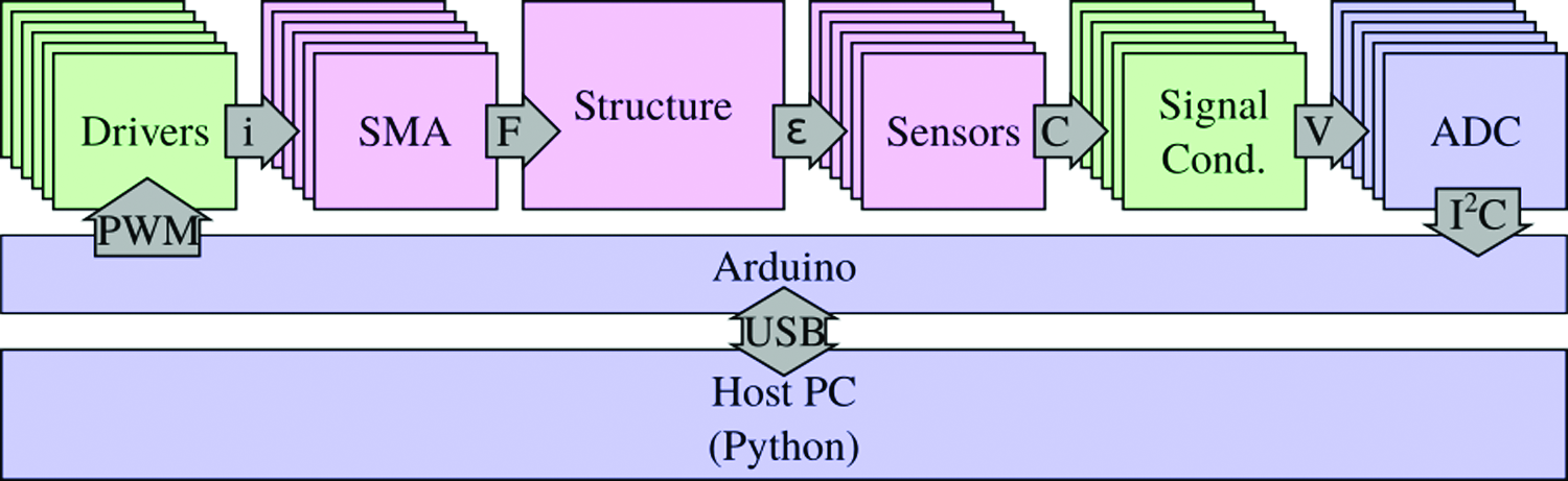
The overall architecture of the electronics of the system, and the ow of data between different modules, is shown in Figure 4. There were two custom-fabricated printed circuit boards used in this project. One was used to provide signal conditioning for the capacitive sensors, and one was used to provide a closed-loop current supply to the SMA actuators. Six of each board were used to control the Stewart platform. Both the sensor signal conditioning and current amplifier modules were based on the PIC16F1825 8-bit microcontroller and MCP6281T quad op amp (Microchip Technologies). All analog filters were implemented by using multiple feedback typology to enable stable operation with greater than unity gain in noninverting operation, which was a requirement imposed by the use of a single-sided voltage supply.
Architecture of the complete soft robotic system. Commercially available components are shown in blue. Customer fabricated circuit boards are shown in green. Fabricated hardware is shown in red. The labels in the arrows describe the type of flow between boxes. Beginning clockwise from left, six PWM voltage signals are passed from the interface Arduino to the SMA drivers. This voltage input signal is converted into a current (i) using a \documentclass{aastex}\usepackage{amsbsy}\usepackage{amsfonts}\usepackage{amssymb}\usepackage{bm}\usepackage{mathrsfs}\usepackage{pifont}\usepackage{stmaryrd}\usepackage{textcomp}\usepackage{portland, xspace}\usepackage{amsmath, amsxtra}\usepackage{upgreek}\pagestyle{empty}\DeclareMathSizes{10}{9}{7}{6}\begin{document}
$$1A / V$$
\end{document} transfer function. The current causes the SMA wire to heat, resulting in a force (F) that is applied to the structure. This force results in a deformation and strain (\documentclass{aastex}\usepackage{amsbsy}\usepackage{amsfonts}\usepackage{amssymb}\usepackage{bm}\usepackage{mathrsfs}\usepackage{pifont}\usepackage{stmaryrd}\usepackage{textcomp}\usepackage{portland, xspace}\usepackage{amsmath, amsxtra}\usepackage{upgreek}\pagestyle{empty}\DeclareMathSizes{10}{9}{7}{6}\begin{document}
$$\epsilon$$
\end{document}) that is measured by the strain sensors, which exhibit a capacitance (C). This capacitance is measured with the signal conditioning electronics, which produce a voltage (V) that is read by ADC. Data from the ADCs are read by the Arduino using the I2C protocol. ADC, analog-to-digital converters; PWM, pulse width modulated. Color images available online at www.liebertpub.com/soro
In the case of the SMA current amplifier, the microcontroller hosted a bang-bang control algorithm. This electronics module contained three filters. The first and second filter were used to filter the analog voltage input and current through the resistive load. The third filter was a differential amplifier that was used to measure the voltage drop across the resistive load. This last filter is not presently implemented, but could be used in the future to control power, rather than current as is presently the case. Current through the SMA wire was controlled via an N-channel depletion-mode MOSFET. To maximize the efficiency of the current driver, this MOSFET was run either fully open or fully closed to reduce ohmic losses within the transistor. The control algorithm applied gate voltage when the filtered SMA current was below the setpoint and turned on the gate voltage when the current was above the setpoint. This combination of filtering and bang-bang control produced a stable response with near-optimal performance for a purely feedback algorithm. The user interface, kinematics solution, and control algorithm were all implemented on a Linux-based PC. Communication between the control software and the electronics was accomplished by using an Arduino Uno R3 microcontroller (Adafruit) and a USB connection. This intermediate controller was responsible for reading the output from the sensor signal conditioning boards by using a 16-bit ADC (ADS1115; Adafruit) and generating eight-bit pulse width modulated (PWM) command signals for the current control boards. The electronics configuration was designed to be stationary and so relies on a relatively bulky PC, individual current drivers, and signal conditioning boards. In the future, an application-specific PCB could be designed and integrated into the structure of the robot to make the overall system more compact.
Testing
To determine the coefficients in Equation (24), we needed to collect output voltage as a function of strain. To do so, we used an Instron 3345 fitted with a 50 N load cell to measure the response of the sensors. As described earlier, the active elastomer sensing element was integrated with rigid tabs to provide an attachment point. The sensors were held by the attachment points in an identical way as they were held when attached to the robot to ensure consistency of results between the Instron testing and on-robot operation. Tests were conducted over operationally representative strain values. Sensors were put through 10 strain cycles to ensure consistent operation.
SMAs have complex thermomechanical responses. We performed two sets of tests to characterize the as-fabricated SMA actuators. The first test was designed to quantify the effect of performance degradation with different applied current and set an upper safe limit on current. Immediately after programming the SMA wire into coils, we used an Instron 3345 materials testing machine fitted with a 50 N load cell to measure the response of the actuators. We applied a 30 mm displacement to simulate pulling the coil to the neutral length when integrated into the robot (i.e., the length shown in Fig. 1). Second, we applied a series of 100 current pulses to the coil, and measured the force generated. The pulses consist of a 20 s on period, followed by a 120 s off period. The results of this test are shown in Figure 6. We conducted these tests at two different current levels, 0.98 and 1.57 A, which correspond to PWM values of 50 and 80 bits, respectively. The second test we conducted on the SMA actuators was to determine the quasi-static response as a function of displacement and applied current. We were interested in displacements from 10 to 50 mm, and applied current values between 10 and 50 bits, which equates to 0.20–0.98 A. To perform this test, we fixed the SMA actuator in the materials testing machine as in the previous test. We created a test grid with all possible combinations and randomly selected trials from this list to mitigate the effects of drift or degradation during the test. For each test condition, we pulled the SMA actuator to the required displacement, and applied a 50-bit pulse of current to activate the coil and remove any slack in the actuator. The data from this initial pulse were not considered in the analysis. Subsequently, we applied three pulses at the required current, using a 20 s on time followed by a 120 s off time. The results of this test are shown in Figure 7.
Once unit testing was complete on the sensors and actuators, we integrated six of each into the complete robotic system. We conducted two tests on the complete robot: an open-loop step response test and a closed-loop response test. In the case of the open-loop test, we applied the same current levels of 10, 20, 30, 40, and 50 bits to each of the six actuators, one actuator at a time, in a random order, and observed the response in the six sensors. As in the component actuator tests, the actuators were turned on for 20 s, and allowed to cool for 120 s. However, unlike the previous actuator tests, there was no “pre-heating” step to remove slack. The actuators were kept taut by the central elastomer structure. Each test condition was evaluated three times. The results of this experiment are shown in Figure 8.
The second trial conducted with the integrated system was a closed-loop test. In this test, a simple per-channel bang-bang controller was implemented with a maximum command of 50 bits. As previously discussed, the controller ran on a PC connected to the robot through an Arduino interface. Each position was held for 60 s. The sequence of commanded states (in absolute coordinates, not relative to the previous state) was neutral, down 3 mm, down 3 mm + roll right 5.62°, down 3 mm + roll right 5.62° + pitch forward 5.62°, down 3 mm + roll right 5.62° + pitch backward 5.62°, down 3 mm, and neutral (for 120 s). This sequence was repeated three times. The results are shown in Figure 9.
Results and Discussion
Sensor performance
One of our goals with this project was to create sensors that were mechanically compatible with the SMA actuators. We have demonstrated that capacitance-based conductive elastomer composite sensors are highly deformable, and therefore have minimal impact on the mechanical characteristics of soft structures to which they are attached. As shown in the force curve of Figure 5, the maximum force observed over the range of operation was less than 1.5 N, which is lower than the maximum force output of the SMA actuators shown in Figure 7 of 4 N. To further decrease the mechanical impact, the sensors could be reduced in width and thickness. This would be easier to implement in integrated sensors than in free-standing sensors such as those we used, since the body to which they are attached would be able to provide mechanical support.
Sensor calibration data. The top two charts show measured voltage and force responses, respectively, as functions of displacement. The bottom chart shows the reconstructed displacement based on a quadratic model. Zero displacement corresponds to the robot in a neutral configuration. Experimental data are shown as dark gray dots, the mean is shown as a black line, and the 95% confidence intervals are shown as gray regions. Data show responses from six sensors over 10 loading/unloading cycles.
We have also demonstrated that a simple film-based approach can be used to easily produce capacitive sensors that can measure strains of the same scale as the SMA actuators. The voltage response of the sensors shown in Figure 5 illustrates the stability of the sensors. The data represent the output from three different sensors, demonstrating that there is good consistency across devices. In addition, we demonstrated that the response of the sensors is stable across many cycles, as shown by the small confidence intervals in both the output voltage and reconstructed displacement curves of Figure 5. Moreover, the voltage output is actually more stable and repeatable than the mechanical response. Based on the observed voltage response, we assumed a quadratic relation between the displacement and voltage. Although Equation (24) shows that the ideal response is linear, we have added a quadratic term to account for non-ideal effects, particularly at large deformation values. We suspect these deviations from a linear response are mostly due to geometric effects within the sensors. To eliminate the effects of buckling, we only considered data in the range \documentclass{aastex}\usepackage{amsbsy}\usepackage{amsfonts}\usepackage{amssymb}\usepackage{bm}\usepackage{mathrsfs}\usepackage{pifont}\usepackage{stmaryrd}\usepackage{textcomp}\usepackage{portland, xspace}\usepackage{amsmath, amsxtra}\usepackage{upgreek}\pagestyle{empty}\DeclareMathSizes{10}{9}{7}{6}\begin{document}
$$d \in [ - 10 , 20 ] \ { \rm{mm}}$$
\end{document}. Using a generalized least-squares approach, we found the response of the sensors to be:
\documentclass{aastex}\usepackage{amsbsy}\usepackage{amsfonts}\usepackage{amssymb}\usepackage{bm}\usepackage{mathrsfs}\usepackage{pifont}\usepackage{stmaryrd}\usepackage{textcomp}\usepackage{portland, xspace}\usepackage{amsmath, amsxtra}\usepackage{upgreek}\pagestyle{empty}\DeclareMathSizes{10}{9}{7}{6}\begin{document}
\begin{align*}
d = \left( {0.152 - 76.9 \Delta V + 59.4 \Delta {V^2}} \right) \pm 1.16 \ { \rm{mm}} , \tag{25}
\end{align*}
\end{document}
where d is the displacement, measured from the neutral position in mm, \documentclass{aastex}\usepackage{amsbsy}\usepackage{amsfonts}\usepackage{amssymb}\usepackage{bm}\usepackage{mathrsfs}\usepackage{pifont}\usepackage{stmaryrd}\usepackage{textcomp}\usepackage{portland, xspace}\usepackage{amsmath, amsxtra}\usepackage{upgreek}\pagestyle{empty}\DeclareMathSizes{10}{9}{7}{6}\begin{document}
$$\Delta V$$
\end{document} is the change in measured voltage, measured in V, and the error represents the 95% confidence interval.
SMA Performance
The limited lifespan of SMA actuators is well established in the literature.45 In addition, SMA actuators are known to have a short transient in performance during the first few cycles. We confirmed both these effects experimentally in the data shown in Figure 6a and b. Moreover, these data show that multiple SMA actuators behave very similarly in Figure 6e and f. To determine the maximum permissible current, we compared the results in Figure 6e and f. In Figure 6e, we saw a pronounced degradation in performance over the first 40 cycles. However, after this initial transient, the force was approximately constant for the remaining cycles. In contrast, in Figure 6f, the force continues to decay over the entire 100 cycle test. Further, the force generated by the higher current test actually produces less force than the lower current test at high numbers of cycles. Therefore, we concluded that a current of 0.98 A (Fig. 6e) was safe for continuous operation. Further supporting this conclusion, we noticed that the response of the first current pulse at the higher 1.57 A setting resulted in degradation during the heating phase as shown in Figure 6b. Instead of increasing in force during the entire heating phase, the trace shows that maximum force was achieved around 10 s, and then began to decay for the remaining 10 s of the pulse. This effect was not observed in any other pulse.
Degradation testing on SMA actuators. (a, b) shows the mechanical response of the first 10 pulses of current at 50 and 80 bits. (c, d) shows 100 pulses, including the first 10. (e, f) shows the maximum force generated as a function of pulse number. Top two rows show data from one actuator coil each, whereas the bottom row shows summary data from three sensors. Color images available online at www.liebertpub.com/soro
Overheating is a significant challenge in SMA actuator design. We want to achieve rapid activation of the coil, which requires rapid heating of the coil, which, in turn, requires high currents. However, high currents also result in steady-state temperatures that are well above the threshold for damaging the actuator coil. Since we cannot directly measure the temperature of the coil in this configuration, we are limited in what information we can provide to the control system. Further, since our response time is dominated by the free convective cooling of the actuators, we conclude that attempting to run the coils with higher currents substantially increases the risk of damage with little improvement to the overall response of the system.
As has been previously reported in the literature,69 we find that the quasi-static force output from the SMA actuators is well modeled by a linear spring model. Figure 7a shows that the force output from the actuator is a function of displacement (top row) and current (bottom row). Further, the figure shows that the effects are approximately linear. Finally, the figure also shows that the slow cooling rate dominates the dynamics of the system. To improve the dynamics response of the system, some way must be found to enhance the cooling rate. We speculate that this might be accomplished by placing the SMA actuators in a thermally conductive environment or by using forced convection.
SMA actuator force as a function of displacement and current. (a) Shows the time history response of a single actuator over three trials in each condition. The top row of images show displacements of 10, 20, 30 (neutral), 40, and 50 mm. Within each figure, data for current commands of 10, 20, 30, 40, and 50 bits are shown as different shades of red. In the second row of images, each plot shows a single current, whereas the different displacements are plotted as different shades of blue. (b, c) Shows the maximum and minimum force exerted by an actuator coil in each condition. The points show the observations from three trials with each of three coils, whereas the surface represents average of the experimental observations at each condition. (d, e) shows the same experimental points as (b, c), but with the surface replaced by the linear approximation. Color images available online at www.liebertpub.com/soro
Returning to Figure 7b, we found that the maximum force generated by the SMA actuator coils was an approximately linear function of the product of displacement and current. In Figure 7c, we found that the minimum force (i.e., residual force in the actuator after the current was turned off) was a function of the displacement, but not the on current. Together, these observations suggested a model of the form:
\documentclass{aastex}\usepackage{amsbsy}\usepackage{amsfonts}\usepackage{amssymb}\usepackage{bm}\usepackage{mathrsfs}\usepackage{pifont}\usepackage{stmaryrd}\usepackage{textcomp}\usepackage{portland, xspace}\usepackage{amsmath, amsxtra}\usepackage{upgreek}\pagestyle{empty}\DeclareMathSizes{10}{9}{7}{6}\begin{document}
\begin{align*}
{ \rm{F ( i , d , }}{{ \rm{d}}_0} ) = ( {K_i}i + {K_0} ) ( d - {d_0} ) , \tag{26}
\end{align*}
\end{document}
where \documentclass{aastex}\usepackage{amsbsy}\usepackage{amsfonts}\usepackage{amssymb}\usepackage{bm}\usepackage{mathrsfs}\usepackage{pifont}\usepackage{stmaryrd}\usepackage{textcomp}\usepackage{portland, xspace}\usepackage{amsmath, amsxtra}\usepackage{upgreek}\pagestyle{empty}\DeclareMathSizes{10}{9}{7}{6}\begin{document}
$$F ( i , d , {d_0} )$$
\end{document} is force applied by the actuator as a function of the applied current i, displacement d, and initial length d0 and ki and k0 are parameters of a linear spring whose stiffness is a function of current. Based on both the maximum and minimum observed force, we determined that these coefficients were \documentclass{aastex}\usepackage{amsbsy}\usepackage{amsfonts}\usepackage{amssymb}\usepackage{bm}\usepackage{mathrsfs}\usepackage{pifont}\usepackage{stmaryrd}\usepackage{textcomp}\usepackage{portland, xspace}\usepackage{amsmath, amsxtra}\usepackage{upgreek}\pagestyle{empty}\DeclareMathSizes{10}{9}{7}{6}\begin{document}
$${K_i} = 1.86 \times {10^{ - 3}}{ \rm{N / mm}}{ \rm{.bit}}$$
\end{document}, \documentclass{aastex}\usepackage{amsbsy}\usepackage{amsfonts}\usepackage{amssymb}\usepackage{bm}\usepackage{mathrsfs}\usepackage{pifont}\usepackage{stmaryrd}\usepackage{textcomp}\usepackage{portland, xspace}\usepackage{amsmath, amsxtra}\usepackage{upgreek}\pagestyle{empty}\DeclareMathSizes{10}{9}{7}{6}\begin{document}
$${K_0} = \; 5.06 \times {10^{ - 3}}{ \rm{N / mm}}$$
\end{document}, and \documentclass{aastex}\usepackage{amsbsy}\usepackage{amsfonts}\usepackage{amssymb}\usepackage{bm}\usepackage{mathrsfs}\usepackage{pifont}\usepackage{stmaryrd}\usepackage{textcomp}\usepackage{portland, xspace}\usepackage{amsmath, amsxtra}\usepackage{upgreek}\pagestyle{empty}\DeclareMathSizes{10}{9}{7}{6}\begin{document}
$${{ \rm{d}}_0} = 2.74{ \rm{mm}}$$
\end{document}. Using this model, we generated estimated maximum and minimum forces in Figure 7d and e, respectively.
The good agreement between the model and the experimental data validates that this approach is sufficient for capturing the quasi-static performance of an SMA actuator without considering the full thermomechanical behavior. Further, this is similar to the approach taken by Holschuh et al., who investigated SMA actuators in a compression garment.69 Given the similar results from two different applications of SMA actuators, we conclude that the reduction to a quasi-static model has utility across a range of applications. At the very least, a quasi-static approach provides a starting point for the design process. Although quasi-static models cannot account for the hysteresis effects in SMAs, they do provide upper bounds on the force that can be generated.
Robot Performance
The open-loop test of robotic system performance is shown in Figure 8. The numbering scheme used in the figure is shown in Figure 2. The sensor data in the vertical axes indicate the internal state vector \documentclass{aastex}\usepackage{amsbsy}\usepackage{amsfonts}\usepackage{amssymb}\usepackage{bm}\usepackage{mathrsfs}\usepackage{pifont}\usepackage{stmaryrd}\usepackage{textcomp}\usepackage{portland, xspace}\usepackage{amsmath, amsxtra}\usepackage{upgreek}\pagestyle{empty}\DeclareMathSizes{10}{9}{7}{6}\begin{document}
$${ \bf{l}}$$
\end{document} from Equation (3). Sensors are arranged into rows, and actuators are arranged into columns. For example, the data in the third row and second column (labeled “S2,A1”) show the response of sensor 2 (“S2”) to the activation of the actuator 1 (“A1”). The sensors and actuators are numbered counterclockwise when looking down at the top of the robotic structure. The data show two effects. First, we see coupling between axes of the robotic system. The diagonal subplots of Figure 8 show each sensor's response to the actuator attached between the same nodes. As expected, the subplots along the diagonal show the maximum deflection. Moving from the diagonal three columns to the left or right, we see the data from the sensor on the opposite side of the structure to the actuator. In these subplots, we see a response of opposite direction to the on-diagonal plots with lower amplitude. Comparing Figure 8 with Figure 6a and c and Figure 7a, we find that the time constants are approximately equal in all situations tested. Since the heating and cooling rates are dictated by the current and free convection, which are constant between tests, this is as expected and indicates that the viscoelasticity of the central elastomer structure plays a negligible role in the dynamics of the system.
Step response from on-board sensors. Each column represents a different actuator. Each row represents a different sensor. Each image contains data from three independent trials. All figures have identical vertical and horizontal axes. Colors represent different current levels, with black being 10 bits ≈0.20 A and red being 50 bits ≈0.98 A. All data collected with 11-tap rolling FIR filter. Red vertical bars at \documentclass{aastex}\usepackage{amsbsy}\usepackage{amsfonts}\usepackage{amssymb}\usepackage{bm}\usepackage{mathrsfs}\usepackage{pifont}\usepackage{stmaryrd}\usepackage{textcomp}\usepackage{portland, xspace}\usepackage{amsmath, amsxtra}\usepackage{upgreek}\pagestyle{empty}\DeclareMathSizes{10}{9}{7}{6}\begin{document}
$$30s$$
\end{document} and \documentclass{aastex}\usepackage{amsbsy}\usepackage{amsfonts}\usepackage{amssymb}\usepackage{bm}\usepackage{mathrsfs}\usepackage{pifont}\usepackage{stmaryrd}\usepackage{textcomp}\usepackage{portland, xspace}\usepackage{amsmath, amsxtra}\usepackage{upgreek}\pagestyle{empty}\DeclareMathSizes{10}{9}{7}{6}\begin{document}
$$50s$$
\end{document} show the times at which the SMA actuators were turned on and off, respectively. The sensor and actuator names are consistent with the labels in Figure 2. FIR, finite impulse response. Color images available online at www.liebertpub.com/soro
The closed-loop test of robotic system performance is shown in Figure 9. The data for the internal state vector \documentclass{aastex}\usepackage{amsbsy}\usepackage{amsfonts}\usepackage{amssymb}\usepackage{bm}\usepackage{mathrsfs}\usepackage{pifont}\usepackage{stmaryrd}\usepackage{textcomp}\usepackage{portland, xspace}\usepackage{amsmath, amsxtra}\usepackage{upgreek}\pagestyle{empty}\DeclareMathSizes{10}{9}{7}{6}\begin{document}
$${ \bf{l}}$$
\end{document} are shown in the top row, data for the configuration state vector \documentclass{aastex}\usepackage{amsbsy}\usepackage{amsfonts}\usepackage{amssymb}\usepackage{bm}\usepackage{mathrsfs}\usepackage{pifont}\usepackage{stmaryrd}\usepackage{textcomp}\usepackage{portland, xspace}\usepackage{amsmath, amsxtra}\usepackage{upgreek}\pagestyle{empty}\DeclareMathSizes{10}{9}{7}{6}\begin{document}
$${ \bf{c}}$$
\end{document} are shown in the middle row, and error data are shown in the bottom row. Commands were received from the operator in configuration space, then converted into internal space as an input to the control loop. The data reported in Figure 9 represent the mean and 95% confidence from three independent trials. The relatively small confidence interval indicates that the robotic system performance is highly repeatable. The relatively large excursions from ideal performance are, therefore, due to system dynamics and material limitations, which are repeatable, rather than from random noise.
Closed-loop tests of the integrated robot system. In all subplots, the red line represents the setpoint, the thin blue line represents the mean of the observation, and the light blue region represents the 95% confidence interval across three trials. The upper row of subplots shows the length states in the vector \documentclass{aastex}\usepackage{amsbsy}\usepackage{amsfonts}\usepackage{amssymb}\usepackage{bm}\usepackage{mathrsfs}\usepackage{pifont}\usepackage{stmaryrd}\usepackage{textcomp}\usepackage{portland, xspace}\usepackage{amsmath, amsxtra}\usepackage{upgreek}\pagestyle{empty}\DeclareMathSizes{10}{9}{7}{6}\begin{document}
$${ \bf{l}}$$
\end{document}. The middle row shows the configuration states of the vector \documentclass{aastex}\usepackage{amsbsy}\usepackage{amsfonts}\usepackage{amssymb}\usepackage{bm}\usepackage{mathrsfs}\usepackage{pifont}\usepackage{stmaryrd}\usepackage{textcomp}\usepackage{portland, xspace}\usepackage{amsmath, amsxtra}\usepackage{upgreek}\pagestyle{empty}\DeclareMathSizes{10}{9}{7}{6}\begin{document}
$${ \bf{c}}$$
\end{document}. The bottom row shows the errors in the configuration states. The first three subplots in the middle and bottom rows are translations in x, y, and z, whereas the second group of three subplots are the rotation components. Color images available online at www.liebertpub.com/soro
The workspace of the robot was limited by the nature of the SMA actuators, which could only apply tension. The effect of this limitation is clearly seen in the first and second internal state vector data between 240 and 300 s (“S0” and “S1” in the top row of Fig. 9), as well as in the fifth and six internal state vector data between 180 and 240 s (“S4” and “S5” in the top row of Fig. 9). At these points in the command history, the required lengths of the actuators exceeded the neutral position length (i.e., >67 mm). For the actuators to have contributed to reducing the error in the system, they would have had to provide extensive force, which is not possible with coiled SMA wire actuators. This situation is illustrated in Figure 10. In this example, the left-hand actuator is fully off and completely cooled. To achieve the commanded position, the actuator would have to extend to \documentclass{aastex}\usepackage{amsbsy}\usepackage{amsfonts}\usepackage{amssymb}\usepackage{bm}\usepackage{mathrsfs}\usepackage{pifont}\usepackage{stmaryrd}\usepackage{textcomp}\usepackage{portland, xspace}\usepackage{amsmath, amsxtra}\usepackage{upgreek}\pagestyle{empty}\DeclareMathSizes{10}{9}{7}{6}\begin{document}
$${l_{l , c}}$$
\end{document}. However, due to the contractive force of the antagonistic actuator on the right side of the figure working in conjunction with the elastomer body, it is only able to extend to \documentclass{aastex}\usepackage{amsbsy}\usepackage{amsfonts}\usepackage{amssymb}\usepackage{bm}\usepackage{mathrsfs}\usepackage{pifont}\usepackage{stmaryrd}\usepackage{textcomp}\usepackage{portland, xspace}\usepackage{amsmath, amsxtra}\usepackage{upgreek}\pagestyle{empty}\DeclareMathSizes{10}{9}{7}{6}\begin{document}
$${l_{l , a}}$$
\end{document}. The extension of the left-hand actuators from their neutral length of \documentclass{aastex}\usepackage{amsbsy}\usepackage{amsfonts}\usepackage{amssymb}\usepackage{bm}\usepackage{mathrsfs}\usepackage{pifont}\usepackage{stmaryrd}\usepackage{textcomp}\usepackage{portland, xspace}\usepackage{amsmath, amsxtra}\usepackage{upgreek}\pagestyle{empty}\DeclareMathSizes{10}{9}{7}{6}\begin{document}
$${l_{l , n}}$$
\end{document} to \documentclass{aastex}\usepackage{amsbsy}\usepackage{amsfonts}\usepackage{amssymb}\usepackage{bm}\usepackage{mathrsfs}\usepackage{pifont}\usepackage{stmaryrd}\usepackage{textcomp}\usepackage{portland, xspace}\usepackage{amsmath, amsxtra}\usepackage{upgreek}\pagestyle{empty}\DeclareMathSizes{10}{9}{7}{6}\begin{document}
$${l_{l , a}}$$
\end{document} is due to the antagonistic effect of the right-hand actuators working in conjunction with elastomer structure. This same effect is observed in both the open- and closed-loop tests. Based on this limitation, we conclude that successful operation of the system is limited to cases where shorter-than-neutral lengths of the actuators are required. To achieve this, one needs to pre-compress the system by using uniform activation of all the actuators. This requirement was another factor that influenced our desire to reduce the stiffness of the central elastomer structure, in addition to the goal of achieving equal stiffness in all axes.
Schematic illustration of the platform commanded to rotate beyond kinematic capability. The neutral position (i.e., the position of the robot with all actuators off), the commanded position, and the achieved position are all shown. The rigid end plates are blue, the central elastomer structure is red, and the actuators are shown schematically as orange lines. Sensors are not shown. In this example, the actuator on the right side is able to achieve the commanded length (i.e., \documentclass{aastex}\usepackage{amsbsy}\usepackage{amsfonts}\usepackage{amssymb}\usepackage{bm}\usepackage{mathrsfs}\usepackage{pifont}\usepackage{stmaryrd}\usepackage{textcomp}\usepackage{portland, xspace}\usepackage{amsmath, amsxtra}\usepackage{upgreek}\pagestyle{empty}\DeclareMathSizes{10}{9}{7}{6}\begin{document}
$${l_{r , a}} = {l_{r , c}}$$
\end{document}), whereas the actuator on the left side is not able to achieve the commanded length (i.e., \documentclass{aastex}\usepackage{amsbsy}\usepackage{amsfonts}\usepackage{amssymb}\usepackage{bm}\usepackage{mathrsfs}\usepackage{pifont}\usepackage{stmaryrd}\usepackage{textcomp}\usepackage{portland, xspace}\usepackage{amsmath, amsxtra}\usepackage{upgreek}\pagestyle{empty}\DeclareMathSizes{10}{9}{7}{6}\begin{document}
$${l_{l , a}} < {l_{l , c}}$$
\end{document}). The left side actuator extended past the neutral length (\documentclass{aastex}\usepackage{amsbsy}\usepackage{amsfonts}\usepackage{amssymb}\usepackage{bm}\usepackage{mathrsfs}\usepackage{pifont}\usepackage{stmaryrd}\usepackage{textcomp}\usepackage{portland, xspace}\usepackage{amsmath, amsxtra}\usepackage{upgreek}\pagestyle{empty}\DeclareMathSizes{10}{9}{7}{6}\begin{document}
$${l_{l , a}} > {l_{l , c}}$$
\end{document}) because of the center elastomer structure and antagonist force from the other actuator. Color images available online at www.liebertpub.com/soro
Another limitation of the workspace is imposed due to the geometry of the system. Looking at the open-loop tests in Figure 8, it appears that the actuators are able to cause a contraction of >10 mm. However, looking at the closed-loop state data, and in particular in the internal state vector data for sensors S2 and S3 (“S2” and “S3” in the top row of Fig. 9), the actuators are only able to achieve ∼5 mm of compression. This is because A2 and A3 are activated simultaneously in the closed-loop tests, as opposed to one at a time in the open-loop test. As a result, in the open-loop test, the actuator is able to pull the two nodes to which it is attached directly toward one another. This results in maximum mechanical efficiency and, hence, maximum contraction. However, in the closed-loop case, when both A2 and A3 are working simultaneously, the corresponding nodes on the upper plate have a relative sideways motion since Nodes 5 and 7 are being pulled down into the gap between Nodes 4 and 6 (see Fig. 2 for node numbers). At high contraction, this results in a near-singular configuration, where the mechanical efficiency of A2 and A3 is much less than unity.
These two configurations are illustrated schematically in Figure 11. As a result, the contraction observed in the closed-loop test is lower than that observed in the open-loop test. The particular command sequence shown in Figure 9 was selected to test this exact phenomenon and demonstrated the limitation of motion in this pathological case.
Schematic illustration of the differences in mechanical advantage between open- and closed-loop tests. The rigid end plates are blue, the central elastomer structure is red, and the actuators are shown schematically as orange lines. Only the two actuators closest to the viewer are shown. In the open-loop tests (upper image), only one actuator was activated at a time. With only one actuator active, the moving plate rotates toward the active actuator attachment point, maintaining mechanical advantage. In the closed-loop test configuration shown, both actuators are on. Because both actuators are pulling, the moving plate rotates down between the actuator attachment points, reducing mechanical advantage relative to the open-loop test. Color images available online at www.liebertpub.com/soro
Looking at the Z translation data (Fig. 9 middle and bottom rows, third column), we can observe the effect of mechanical coupling between actuators. During the period between 120 and 300 s, we observe that the moving platform drops below the setpoint value every 60 s, when a new angular configuration is commanded. This occurs because the cooling rate of the SMA actuators is slower than the heating rate. Because of this, actuators on both sides of the structure were applying a contractive force: The actuators from the previous cycle were still “on” and cooling to below their activation temperature, whereas the actuators for the current cycle were also commanded “on.” As the deactivated SMA actuators cooled, the error in Z translation decreased until the system achieved zero error, which was typically in about 30 s. This effect was, in part, an artifact of our control strategy. Instead of controlling the translation and rotation states, we controlled the sensor lengths. As such, the control algorithm was unaware of the deviations in Z translation, and no effort was made to correct the error.
We utilized a simple bang-bang controller architecture with a single control loop attached to each internal state. Outside of the workspace limitations discussed earlier, once the system achieves a zero-error condition, the controller is able to maintain the system at that location as shown by the stable regions in the bottom row of Figure 9. Controllers of this type are subject to “chatter,” particularly in cases of noisy observations, which we observed in the small oscillations in the error traces. We believe that more advanced controllers, particularly a control architecture employing fuzzy logic, could be implemented in the future to enhance the performance of the robotic system. Further, by implementing a controller with lower noise sensitivity, we would be able to increase the maximum current in the system without increasing the risk of overheating, which would improve performance. In addition, our current approach relies exclusively on feedback. Given the long time delays associated with SMA actuators, we suggest that model-based feedforward controllers could provide better performance, particularly if the mechanical coupling between SMA actuators was considered in the model.
The maximum current used in this system was limited by the danger of overheating the SMA actuators. We chose a maximum current based on steady-state heating. However, pulse heating can also be used with SMA actuators where an initial pulse is provided to rapidly heat the coils. Without state feedback from the SMA wire, this approach can overheat the coils and cause degradation. More than just temperature feedback is required. In addition, the current loading condition, and an estimate of the internal composition of the SMA wire (i.e., percentage of martensite) are needed to ensure that the thermodynamic conditions remain below the degradation point. This is very difficult to achieve in practice. Further, this only solves the heating problem. As noted earlier, cooling rate is just as important to overall system performance. Since this is currently a passive process, we are limited in our options. We suggest that improved heat transfer rates, through either forced convection or enhanced conduction into a higher heat capacity medium, such as water, could address both challenges simultaneously. However, adding a fluidic temperature control system would present a new set of integration and fabrication challenges.
Conclusion
In this article, we have described the manufacturing, integration, and testing of a soft robotic structure. Like many soft robots, the functionality of our system is based on the responsive materials from which the robot is fabricated. We relied on nickel-titanium SMA wire as an actuator material, and we determined the maximum current that could be used for actuation without damaging the actuators. We also collected data to support a quasi-static force and displacement model of the coiled actuators, which we used for design purposes. Finally, we determined the dynamic response of the isolated SMA actuators and compared this with the dynamic response of the integrated robot. We concluded that the dynamics of the system was driven by the actuators, and not by the material properties of the sensors or central elastomer structure. To provide state feedback, we also developed a conductive elastomer composite material and created highly deformable strain gauges from deformable capacitive structures. We developed an analytic model of these sensors, including the operation of the readout electronics, and compared the results with experimental data. From our experimental data, we characterized the repeatability of the sensors and the accuracy. Finally, we created an experimentally anchored calibration curve that we used in the integrated robotic system. We integrated six sensors and actuators together to provide full six DoF state control in an elastomer-based robotic system. We defined a series of internal states corresponding to the lengths of each sensor, then actively controlled these lengths to achieve position control. Since these internal states are not intuitive and are difficult to use to express the kinematics of the system, we also described the mapping and its inverse between the internal states and a more intuitive translation-rotation state formulation. All of the commands we gave to the robotic system were in terms of the intuitive states, which were then converted into the internal states for input to the control loops. We were able to demonstrate highly repeatable controlled motion of the robotic system.
In the future, we intend to continue to refine the material-level models of the responsive materials, particularly of the actuator. We believe that the future of soft robot development requires an enhanced understanding of the interactions between responsive materials elements, which, in turn, requires the development of integrated models that can be used for design and analysis purposes. In this article, we assembled our soft system from discrete responsive material components. Our long-term goal is to create complete soft robotic systems from heterogeneous responsive and traditional materials through advanced manufacturing processes, such as 3D printing and molding, without any assembly steps. To achieve this level of integration, we will need to progress through our current assembled prototype phase into a field with better models and design tools.
Footnotes
Acknowledgments
This work is partially supported under the NASA Early Career Faculty Program, Space Technology Research Grants Program (Grant NNX14AO52G). E.L.W. is supported by the National Science Foundation Graduate Research Fellowship (Grant DGE-1333468). J.C.C. is supported by the National Aeronautics and Space Administration Space Technology Research Fellowship (NNX15AQ75H). Any opinion, findings, and conclusions or recommendations expressed in this material are those of the authors and do not necessarily reflect the views of the National Science Foundation or the National Aeronautics and Space Administration.
Author Disclosure Statement
No competing financial interests exist.
References
1.
LaschiC. Soft Robotics: from scientific challenges to technological applications. In GeorgeT, DuttaAK, Saif IslamM (Eds), Proceedings of the SPIE, Vol. 9836, Baltimore, MD, USA, 2016, p. 983626.
2.
LaschiC, CianchettiM. Soft robotics: new perspectives for robot bodyware and control. Front Bioeng Biotechnol, 2014; 2:3.
3.
MarcheseAD, KatzschmannRK, RusD. A recipe for soft fluidic elastomer robots. Soft Robot, 2015; 2:7–25.
4.
RusD, TolleyMT. Design, fabrication and control of soft robots. Nature, 2015; 521:467–475.
StewartD. A platform with six degrees of freedom. Archive Proc Inst Mech Eng 1847–1982 (Vols. 1–196), 1965; 180:371–386.
7.
CalistiM, ArientiA, RendaF, LevyG, HochnerB, MazzolaiB, et al.Design and development of a soft robot with crawling and grasping capabilities. In 2012 IEEE International Conference on Robotics and Automation (ICRA), St. Paul, MN, USA, 2012, pp. 4950–4955.
8.
LiT, NakajimaK, CianchettiM, LaschiC, PfeiferR. Behavior switching using reservoir computing for a soft robotic arm. In 2012 IEEE International Conference on Robotics and Automation (ICRA), St. Paul, MN, USA, 2012, pp. 4918–4924.
9.
GiorelliM, RendaF, CalistiM, ArientiA, FerriG, LaschiC. Learning the inverse kinetics of an octopus-like manipulator in three-dimensional space. Bioinspir Biomim, 2015; 10:035006.
10.
MarcheseAD, KomorowskiK, OnalCD, RusD. Design and control of a soft and continuously deformable 2d robotic manipulation system. In 2014 IEEE International Conference on Robotics and Automation (ICRA), Hong Kong, China, 2014, pp. 2189–2196.
11.
MarcheseAD, RusD. Design, kinematics, and control of a soft spatial fluidic elastomer manipulator. Int J Robot Res, 2015; 29:242–245.
12.
CaseJC, WhiteEL, KramerRK. Sensor enabled closed-loop bending control of soft beams. Smart Mater Struct, 2016; 25:045018.
13.
LuoM, PanY, SkorinaEH, TaoW, ChenF, OzelS, et al.Slithering towards autonomy: a self-contained soft robotic snake platform with integrated curvature sensing. Bioinspir Biomim, 2015; 10:055001.
IlievskiF, MazzeoAD, ShepherdRF, ChenX, WhitesidesGM. Soft robotics for chemists. Ang Chem Int Ed, 2011; 50:1890–1895.
16.
MartinezRV, BranchJL, FishCR, JinL, ShepherdRF, NunesRMD, et al.Robotic tentacles with three-dimensional mobility based on flexible elastomers. Adv Mater, 2013; 25:205–212.
17.
SkorinaEH, TaoW, ChenF, LuoM, OnalCD. Motion control of a soft-actuated modular manipulator. In 2016 IEEE International Conference on Robotics and Automation (ICRA), Stockholm, Sweden, 2016, pp. 4997–5002.
18.
DasguptaB, MruthyunjayaTS. The Stewart platform manipulator: a review. Mech Mach Theory, 2000; 35:15–40.
19.
HadiA, Yousefi-KomaA, MoghaddamMM, ElahiniaM, GhazaviA. Developing a novel SMA-actuated robotic module. Sens Actuators A Phys, 2010; 162:72–81.
20.
RoslanAMBS, AmirthamV, NagarajanT, HashimFM. SMA actuator technology application in Stewart platform construction. J Appl Sci, 2011; 11:3783–3790.
21.
DunlopR, GarciaAC. A nitinol wire actuated stewart platform. In Proceedings of 2002 Australasian Conference on Robotics and Automation, Auckland, New Zealand, November 2002.
22.
HadiA, AkbariH, TarvirdizadehB, AlipourK. Developing a novel continuum module actuated by shape memory alloys. Sens Actuators A Phys, 2016; 243:90–102.
23.
CaseJ, YuenM, MohammedM, KramerR. Sensor skins: an overview. In RogersJA, GhaffariR, KimD-H (Eds). Stretchable Bioelectronics for Medical Devices and Systems. Cham: Springer International Publishing, 2016, pp. 173–191.
24.
ParkM, ParkJ, JeongU. Design of conductive composite elastomers for stretch-able electronics. Nano Today, 2014; 9:244–260.
25.
ChiechiRC, WeissEA, DickeyMD, WhitesidesGM. Eutectic gallium indium (EGaIn): a moldable liquid metal for electrical characterization of self-assembled mono-layers. An Chemie, 2008; 120:148–150.
26.
KramerRK, MajidiC, WoodRJ. Wearable tactile keypad with stretchable artificial skin. In 2011 IEEE International Conference on Robotics and Automation (ICRA), Shanghai, China, 2011, pp. 1103–1107.
27.
MajidiC, KramerR, WoodRJ. A non-differential elastomer curvature sensor for softer-than-skin electronics. Smart Mater Struct, 2011; 20:105017.
28.
KramerRK, MajidiC, SahaiR, WoodRJ. Soft curvature sensors for joint angle proprioception. In 2011 IEEE/RSJ International Conference on Intelligent Robots and Systems (IROS), San Francisco, CA, USA, 2011, pp. 1919–1926.
29.
ParkY-L, MajidiC, KramerR, BrardP, WoodRJ. Hyperelastic pressure sensing with a liquid-embedded elastomer. J Micromech Microeng, 2010; 20:125029.
30.
HammondFL, KramerRK, WanQ, HoweRD, WoodRJ. Soft tactile sensor arrays for micromanipulation. In 2012 IEEE/RSJ International Conference on Intelligent Robots and Systems (IROS), Vilamoura, Portugal, 2012, pp. 25–32.
31.
ParkY-L, ChenB-R, WoodRJ. Soft artificial skin with multi-modal sensing capability using embedded liquid conductors. In 2011 IEEE Sensors, Limerick, Ireland, 2011, pp. 81–84.
32.
ParkY-L, ChenB-R, WoodRJ. Design and fabrication of soft artificial skin using embedded microchannels and liquid conductors. IEEE Sens J, 2012; 12:2711–2718.
33.
ParkY-L, WoodRJ. Smart pneumatic artificial muscle actuator with embedded microuidic sensing. In 2013 IEEE Sensors, Baltimore, MD, USA, 2013, pp. 1–4.
34.
BilodeauRA, WhiteEL, KramerRK. Monolithic fabrication of sensors and actuators in a soft robotic gripper. In 2015 IEEE/RSJ International Conference on Intelligent Robots and Systems (IROS), Hamburg, Germany, 2015, pp. 2324–2329.
35.
FarrowN, CorrellN. A soft pneumatic actuator that can sense grasp and touch. In 2015 IEEE/RSJ International Conference on Intelligent Robots and Systems (IROS), Hamburg, Germany, 2015, pp. 2317–2323.
36.
WhiteE, CaseJ, KramerR. Multi-element strain gauge modules for soft sensory skins. IEEE Sens J, 2015; 1–1.
37.
CottonDPJ, GrazIM, LacourSP. A multifunctional capacitive sensor for stretchable electronic skins. IEEE Sens J, 2009; 9:2008–2009.
38.
CaiL, SongL, LuanP, ZhangQ, ZhangN, GaoQ, et al.Super-stretchable, transparent carbon nanotube-based capacitive strain sensors for human motion detection. Sci Rep, 2013; 3.
39.
SadasivuniKK, PonnammaD, ThomasS, GrohensY. Evolution from graphite to graphene elastomer composites. Prog Polym Sci, 2014; 39:749–780.
40.
KujawskiM, PearseJD, SmelaE. Elastomers filled with exfoliated graphite as compliant electrodes. Carbon, 2010; 48:2409–2417.
JaniJM, LearyM, SubicA, GibsonMA. A review of shape memory alloy research, applications and opportunities. Mater Des, 2014; 56:1078–1113.
46.
JacksonCM, WagnerHM, WasilewskiRJ. 55-Nitinol-The Alloy with a Memory: It's Physical Metallurgy Properties, and Applications. NASA SP-5110. Jena, Germany; NASA Special Publication, 1972, p. 5110.
47.
OtsukaK, RenX. Recent developments in the research of shape memory alloys. Intermetallics, 1999; 7:511–528.
48.
SreekumarM, NagarajanT, SingaperumalM, ZoppiM, MolfinoR. Critical review of current trends in shape memory alloy actuators for intelligent robots. Ind Robot, 2007; 34:285–294.
49.
BellouardY. Shape memory alloys for microsystems: a review from a material research perspective. Mater Sci Eng A, 2008; 481482:582–589.
50.
PaikJK, KramerRK, WoodRJ. Stretchable circuits and sensors for robotic origami. In 2011 IEEE/RSJ International Conference on Intelligent Robots and Systems (IROS), San Francisco, CA, USA, 2011, pp. 414–420.
51.
YuenM, CherianA, CaseJC, SeipelJ, KramerRK. Conformable actuation and sensing with robotic fabric. In 2014 IEEE/RSJ International Conference on Intelligent Robots and Systems (IROS 2014), Chicago, IL, USA, 2014, pp. 580–586.
52.
MenciassiA, GoriniS, PernorioG, WeitingL, ValvoF, DarioP. Design, Fabrication and Performances of a Biomimetic Robotic Earthworm. In IEEE International Conference on Robotics and Biomimetics (ROBIO) 2004, Shenyang, China, 2004, pp. 274–278.
53.
KimB, LeeMG, LeeYP, KimY, LeeG. An earthworm-like micro robot using shape memory alloy actuator. Sens Actuators A Phys, 2006; 125:429–437.
54.
KohJ-S, ChoK-J. Omegabot: biomimetic inchworm robot using SMA coil actuator and smart composite microstructures (SCM). In 2009 IEEE International Conference on Robotics and Biomimetics (ROBIO), Guilin, China, 2009, pp. 1154–1159.
55.
WangZ, HangG, LiJ, WangY, XiaoK. A micro-robot fish with embedded SMA wire actuated fexible biomimetic fin. Sens Actuators A Phys, 2008; 144:354–360.
56.
WangZ, WangY, LiJ, HangG. A micro biomimetic manta ray robot fish actuated by SMA. In 2009 IEEE International Conference on Robotics and Biomimetics (ROBIO), Guilin, China, 2009, pp. 1809–1813.
57.
MaoS, DongE, ZhangS, XuM, YangJ. A new soft bionic starfish robot with multi-gaits. In 2013 IEEE/ASME International Conference on Advanced Intelligent Mechatronics (AIM), Wollongong, NSW, Australia, 2013, pp. 1312–1317.
58.
KimH-J, SongS-H, AhnS-H. A turtle-like swimming robot using a smart soft composite (SSC) structure. Smart Mater Struct, 2013; 22:014007.
59.
ChengN, IshigamiG, HawthorneS, ChenH, HansenM, TelleriaM, et al.Design and analysis of a soft mobile robot composed of multiple thermally activated joints driven by a single actuator. In 2010 IEEE International Conference on Robotics and Automation (ICRA), Anchorage, AK, USA, 2010, pp. 5207–5212.
60.
SugiyamaY, HiraiS. Crawling and jumping by a deformable robot. Int J Robot Res, 2006; 25:603–620.
IkutaK, TsukamotoM, HiroseS. Shape memory alloy servo actuator system with electric resistance feedback and application for active endoscope. In Proceedings of 1988 IEEE International Conference on Robotics and Automation, Philadelphia, PA, USA, 1988, Vol. 1, pp. 427–430.
63.
IkutaK. Micro/miniature shape memory alloy actuator. In Proceedings of 1990 IEEE International Conference on Robotics and Automation, Cincinnati, OH, USA, 1990, Vol. 3, pp. 2156–2161.
64.
IkutaK, TsukamotoM, HiroseS. Mathematical model and experimental verification of shape memory alloy for designing micro actuator. In Proceedings of the IEEE Micro Electro Mechanical Systems, 1991, MEMS ’91, An Investigation of Micro Structures, Sensors, Actuators, Machines and Robots, Nara, Japan, 1991, pp. 103–108.
65.
MajimaS, KodamaK, HasegawaT. Modeling of shape memory alloy actuator and tracking control system with the model. IEEE Trans Control Syst Technol, 2001; 9:54–59.
66.
AlexandreR, de AguiarA, SaviMA,. Shape Memory alloy helical springs performance: modeling and experimental analysis. Mater Sci Forum, 2013; 758:147–156.
67.
AnS-M, RyuJ, ChoM, ChoK-J. Engineering design framework for a shape memory alloy coil spring actuator using a static two-state model. Smart Mater Struct, 2012; 21:055009.
68.
SeokS, OnalCD, ChoK-J, WoodRJ, RusD, KimS. Meshworm: a peristaltic soft robot with antagonistic nickel titanium coil actuators. IEEE/ASME Trans Mechatronics, 2013; 18:1485–1497.
69.
HolschuhB, NewmanD. Two-spring model for active compression textiles with integrated NiTi coil actuators. Smart Mater Struct, 2015; 24:035011.