Simulating Soft-Bodied Swimmers with Particle-Based Physics

Abstract

In swimming virtual creatures, there is often a disparity between the level of detail in simulating a swimmer's body and that of the fluid it moves in. To address this disparity, we have developed a new approach to modeling swimming virtual creatures using pseudo-soft bodies and particle-based fluids, which has sufficient realism to investigate a larger range of body–environment interactions than are usually included. As this comes with increased computational costs, which may be severe, we have also developed a means of reducing the volume of fluid that must be simulated.

Introduction

Various kinds of simulations are playing an increasingly important role in robotics, allowing preliminary investigations of physical designs and control techniques before committing to the construction of a real world device. Soft robotics is no exception to this trend. Indeed, within some approaches, notably those applying evolutionary robotics¹ methodologies, it is a necessity. The vast numbers of potential solutions that are evaluated in such population based methods, in the search for a highly fit design, mean that simulation-based fitness evaluations are required.

The way in which bodies influence movement and can perform computation, often referred to as morphological computation,^2,3 is particularly relevant to soft robots, as well as being recognized as key to understanding the genesis of natural adaptive behavior. Exploiting subtle interactions between body, environment, and controller can provide powerful ways to generate behavior, but at the same time presents severe challenges to traditional design methodologies. It is very difficult to foresee how these interactions will play out, especially when trying to develop robots that fulfil one or more design criteria (e.g., efficiency). Hence an important developing avenue of investigation in soft robotics is the use of automated evolutionary approaches, which involve the coevolution of brains and bodies, and their interactions with environments.^4–6

One area where many interesting opportunities arise to exploit morphological computation involves soft bodied swimmers acting in aquatic environments, not least because of the relative complexity of the body–environment interactions. This is an area rich with potential application in soft robotics,^6,7 as well as one that might generate fundamental insights into biological behavior.⁸

This trade-off is especially apparent in the simulation of soft-bodied swimmers due to the complexity of accurately simulating fluid dynamics and their interactions with a deformable body, where the goal is to create sufficient realism with as low a cost as possible. Evolutionary robotics methodologies such as minimal simulations⁹ have been well applied to minimizing computational costs when generating controllers for robots with fixed body plans, but such approaches are more difficult to apply when controllers and body plans are coevolved. In general, the less that the body plan is constrained, the less can be predicted about the interactions between the body and the environment, and the more detailed the physics of a simulation must be if realistic behaviors are to be observed.

In this study, we therefore introduce a new method for studying the role of morphology in behavior by simulating swimming agents with soft bodies, which increases the realism of body–environment interactions over earlier methods for swimming virtual creatures, and we also present a means of minimizing the computational cost imposed by the use of this method.

Although the physics of bodies in virtual creatures and simulated soft robots has moved on significantly since they were first introduced by Sims,¹⁰ the physics of fluids for swimming virtual creatures has not. The model used by Sims as long ago as 1994, the model introduced by Sfakiotakis and Tsakiris,¹¹ and also used by authors, including Schramm and Sendhoff¹² and Joachimczak et al.,⁷ and that of Corucci et al.⁶ from 2018 are all much the same. Sfakiotakis and Tsakiris have pointed out that their model is suitable for only certain types of swimming, as it neglects certain interactions between a swimmer's body and a surrounding fluid which are found in nature:

Because the assumptions of this fluid drag model restrict its scope to the inviscid swimming of elongated animals, it cannot be applied to the undulatory swimming of microorganisms (e.g., nematodes), nor to the more sophisticated swimming modes encountered in fish.¹¹

This highlights a disparity between the elements of simulation used by some of the authors above, especially in the recent work by Corucci et al.,⁶ where a highly sophisticated physics engine, Voxelyze,^13,14 is used to simulate the soft bodies of the swimming virtual creatures, but is paired with a relatively simplistic fluid model. To address this disparity, we have developed a new approach to modeling swimming virtual creatures using pseudo-soft bodies and particle-based fluids, which has sufficient realism to investigate a larger range of body–environment interactions. As this comes with increased computational costs, which may be severe, we have also developed a means of reducing the volume of fluid that must be simulated.

We have implemented three models for interactions between swimmers and water: two using particle-based physics and a third, for comparison, which uses the fluid drag model of Sfakiotakis and Tsakiris.¹¹ The first particle-based environment simulates a full water tank and is implemented because it allows for a larger set of agent–environment interactions than the fluid drag model. The second simulates a smaller volume of water, which moves with the swimmer, allowing an environment of arbitrary size to be modeled with a relatively constant computational cost. To test and compare our model environments, we implemented two swimmers, which are designed to exploit two different classes of body–environment interaction. The first, achieved through the use of a novel pseudo-soft body method, swims by pushing against the fluid which surrounds it. The second is jet-propelled and propels itself forwards by expelling the fluid from its body.

This article is structured as follows: we will begin by describing our simulation methods, environmental models, and swimmer designs in the Methods section, followed by the results of running the simulation in Results section, and some analysis of the body–environment interactions which enable one of our swimmers to turn and to propel itself through the water in the particle-based environments in Motion Analysis section. Finally, we will close the article with an evaluation of the three environments and some considerations of future directions in Discussion section.

Methods

In this section, we describe the different models that we implemented for modeling interactions between swimmers and water and the swimmers and controllers that we used to test them. We also describe our method for simulating actuated soft bodies using only rigid body physics, which was necessitated by the use of particle-based fluids.^*

Environments

Full particle-based simulation (tank)

We used Google's liquidfun,¹⁵ a two-dimensional physics engine library in the C++ language, which extends Box2D, as the basis of this simulation. We selected liquidfun as it adds soft bodies and fluids, both implemented with particle-based physics, to the rigid bodies already present in Box2D. We describe the mechanics of the particle physics in Supplementary Data. For our first simulation environment, we simulated a tank full of water by building a square-shaped enclosure of rigid bodies and filling it with a particle-based fluid (Fig. 1). The particles used in both of our particle-based environments are of the water particle type, with radius 0.125 m and a density of 0.005 kg/m². These parameter values were arrived at for the following reasons: although its units are essentially arbitrary, dimensions in Box2D are labelled as SI units and we have retained that convention.

FIG. 1.

The full particle-based fluid simulation, with a tank containing the simulated water, seen in a screen capture from a simulation debugging window. A triangular swimmer can be seen in the tank, and the chemical gradient, depicted by the background tone, is centered on the center of the tank.

Box2D's physics for rigid bodies and the various joints which may connect them can become unstable at very small scales, and so to avoid this problem, our first swimmer's body, described in A Pseudo-Soft Body section, has a side length of 2 m. The scale of the swimmer being set, the particle dimensions were obtained by trial and error, with the competing objectives of realistic fluid–body interactions (assessed only by visual inspection so far) and computational performance in mind. In particular, if particle radii are too large, we cannot expect realism, as the fluid will be made of large balls which only make contact with the swimmer's body at a small number of points, but if, on the other hand, they are too small, their number will be much larger, which will impact heavily on performance. In liquidfun, particles are grouped into systems.

Initially, we found that in our water particle system, the pressure was too low to accommodate swimming. We countered this problem by defining a system with two water particle groups, which elevate the pressure by mixing together. We used a simulation interval of 1 ms, for stability and realistic rigid body and fluid interactions. In this interval, a single iteration is specified for each of velocity, position, and particle iterations.

Reduced particle-based simulation (particle cloud)

For a given density of a particle system, the number of particles to be simulated is directly proportional to the area they fill. The computational cost of a particle system cannot be precisely predicted, as, for a given number of particles, the computational cost of simulation is variable, depending on how much energy there is in the system. Nevertheless, as area is related to the square of distance, so the relationship between the scale of a particle system and its computational cost is an approximately quadratic one. This being the case, significant performance gains can be made by minimizing the scale of a particle system.

We begin with the assumption that for any particle or body there will be some distance beyond which the surrounding particles have only a negligible effect (see Fig. 14 for an illustration). Based on this assumption, the first step in our particle count minimization was to define a system of particles in only a subregion of the tank, centered about the swimmer, and moving with it (Fig. 2). Notionally, this system is square shaped, and the particles are prevented from dissipating and escaping the system by exerting an inward force on any particles which travel outwards beyond the boundary. In practice, the forces are kept as small as possible, so as not to cause large turbulent effects, and so only weakly constrain the shape of the particle system. An issue which we discovered during the development of this method is that a positive feedback loop can form between the motion of the swimmer and that of the particle system.

FIG. 2.

The reduced particle system or particle cloud. To enable quick development with a relatively fast simulation, only a small region of the simulated world, centered on the swimmer's body, contains particles. The particles are free to move within the square-shaped region, but the boundary moves with the swimmer.

As the boundary changes position with the swimmer, it can also effectively cause a current in the direction of the swimmer's travel, increasing the swimmer's motion, and so on. This is particularly noticeable when the swimmer is passively drifting.

To counteract this effect, we artificially induce a current flowing in a direction approximately opposed to the swimmer's motion (Fig. 3). At the beginning of every simulation step, a randomly selected particle is deleted and a replacement created outside the particle system, in front of one of the edges which the swimmer is moving toward. As the replacement particles are driven into the system by the aforementioned confining force, the particle system is internally agitated. When the swimmer is moving in a relatively straight and quick manner, an opposing current in the particle system can be observed. As the rate of input of new particles to the system is constant, rather than based on the speed the system moves at, when the swimmer is moving slowly or with less clear direction, a more turbulent effect can be seen (Fig. 4).

FIG. 3.

As the swimmer moves, the particle system is loosely constrained to track its position. Newly created particles and particles which are found outside the boundary due to either their own movement or that of the swimmer have a force applied to restore them to the defined area. The forces are kept as small as possible, so as not to cause large turbulent effects, and so only weakly constrain the shape of the particle system. The color of new particles periodically alternates between black and white so that currents can be observed. Although it is not easily seen in a single frame, when the swimmer is swimming in a reasonably straight line a current opposing its motion can often be observed. The gray and white traces behind the swimmer indicate the positions of its front node and center of mass, respectively, over time. Supplementary Videos S1-S5 show the actions of the triangular swimmers.

FIG. 4.

When swimmer B gets close to the source of the gradient, it ceases to change position, but tends to rotate on the spot. At this point, the flows in the particle system become more turbulent, most clearly evident from the way the boundary becomes more irregular.

Overall, although there are some differences between the dynamics of the particle cloud simulation and one where a tank full of particles are simulated, they are similar enough that it appears that most, if not all, combinations of swimmer parameters and control structures which prove effective in the particle cloud environment also prove effective in the other. Indeed, although it is possible that there will be effects present in the particle cloud but not in the full simulation which a swimmer's performance depends upon, in general the artificially induced current appears to make the particle cloud the more challenging of the two environments, meaning that a swimmer that succeeds in its task in the particle cloud should also succeed in the larger particle system.

One final problem arose from the fact that the plane of operation of our swimmer is perpendicular to the axis of gravity, which is to say that the simulated particles are unaffected by gravity. This results in the particle system having low pressure and as a result being highly compressible. For the triangular swimmer, this can mean that not all of the exterior of the swimmer is in contact with the water at all times, as the particles which are pushed outwards in the expansion phase return too slowly during the contraction phase.

To counteract this effect, and artificially increase water pressure, the particle cloud is constrained in an area which is approximately half of the area it is instantiated in. Although this solution works for the triangular swimmer, when we added a jet-propelled swimmer, which relies on a different class of body–environment interactions to travel, we discovered that the pressure is still not sufficient to support certain swimming styles (this is described in Jet-Propelled Swimming section).

Drag

We based our fluid drag model on that of Sfakiotakis and Tsakiris.¹¹ The force equations for a single face in contact with the water are: \documentclass{aastex}\usepackage{amsbsy}\usepackage{amsfonts}\usepackage{amssymb}\usepackage{bm}\usepackage{mathrsfs}\usepackage{pifont}\usepackage{stmaryrd}\usepackage{textcomp}\usepackage{portland, xspace}\usepackage{amsmath, amsxtra}\usepackage{upgreek}\pagestyle{empty}\DeclareMathSizes{10}{9}{7}{6}\begin{document} \begin{align*} {F_T} = - { \lambda _T}sgn ( {v_T} ) \cdot { ( {v_T} ) ^2} \tag{1} \end{align*} \end{document} \documentclass{aastex}\usepackage{amsbsy}\usepackage{amsfonts}\usepackage{amssymb}\usepackage{bm}\usepackage{mathrsfs}\usepackage{pifont}\usepackage{stmaryrd}\usepackage{textcomp}\usepackage{portland, xspace}\usepackage{amsmath, amsxtra}\usepackage{upgreek}\pagestyle{empty}\DeclareMathSizes{10}{9}{7}{6}\begin{document} \begin{align*} {F_N} = - { \lambda _N}sgn ( {v_N} ) \cdot { ( {v_N} ) ^2} \tag{2} \end{align*} \end{document}

where F_T is the drag force tangential to the face, and F_N is the drag force in the axis normal to the face. The drag coefficients \documentclass{aastex}\usepackage{amsbsy}\usepackage{amsfonts}\usepackage{amssymb}\usepackage{bm}\usepackage{mathrsfs}\usepackage{pifont}\usepackage{stmaryrd}\usepackage{textcomp}\usepackage{portland, xspace}\usepackage{amsmath, amsxtra}\usepackage{upgreek}\pagestyle{empty}\DeclareMathSizes{10}{9}{7}{6}\begin{document} $${ \lambda _T}$$ \end{document} and \documentclass{aastex}\usepackage{amsbsy}\usepackage{amsfonts}\usepackage{amssymb}\usepackage{bm}\usepackage{mathrsfs}\usepackage{pifont}\usepackage{stmaryrd}\usepackage{textcomp}\usepackage{portland, xspace}\usepackage{amsmath, amsxtra}\usepackage{upgreek}\pagestyle{empty}\DeclareMathSizes{10}{9}{7}{6}\begin{document} $${ \lambda _N}$$ \end{document} are calculated using the following equation: \documentclass{aastex}\usepackage{amsbsy}\usepackage{amsfonts}\usepackage{amssymb}\usepackage{bm}\usepackage{mathrsfs}\usepackage{pifont}\usepackage{stmaryrd}\usepackage{textcomp}\usepackage{portland, xspace}\usepackage{amsmath, amsxtra}\usepackage{upgreek}\pagestyle{empty}\DeclareMathSizes{10}{9}{7}{6}\begin{document} \begin{align*} \lambda = \frac { 1 } { 2 } \rho Cl \tag { 3 } \end{align*} \end{document}

where \documentclass{aastex}\usepackage{amsbsy}\usepackage{amsfonts}\usepackage{amssymb}\usepackage{bm}\usepackage{mathrsfs}\usepackage{pifont}\usepackage{stmaryrd}\usepackage{textcomp}\usepackage{portland, xspace}\usepackage{amsmath, amsxtra}\usepackage{upgreek}\pagestyle{empty}\DeclareMathSizes{10}{9}{7}{6}\begin{document} $$\rho$$ \end{document} is fluid density, C is a shape coefficient, and l is the length of the face.

As all the coefficients in the equation for \documentclass{aastex}\usepackage{amsbsy}\usepackage{amsfonts}\usepackage{amssymb}\usepackage{bm}\usepackage{mathrsfs}\usepackage{pifont}\usepackage{stmaryrd}\usepackage{textcomp}\usepackage{portland, xspace}\usepackage{amsmath, amsxtra}\usepackage{upgreek}\pagestyle{empty}\DeclareMathSizes{10}{9}{7}{6}\begin{document} $$\lambda$$ \end{document} have only linear (scaling) effect on the drag dynamics, for the particular tests we perform here they are arbitrary. For \documentclass{aastex}\usepackage{amsbsy}\usepackage{amsfonts}\usepackage{amssymb}\usepackage{bm}\usepackage{mathrsfs}\usepackage{pifont}\usepackage{stmaryrd}\usepackage{textcomp}\usepackage{portland, xspace}\usepackage{amsmath, amsxtra}\usepackage{upgreek}\pagestyle{empty}\DeclareMathSizes{10}{9}{7}{6}\begin{document} $${ \lambda _T}$$ \end{document} we set \documentclass{aastex}\usepackage{amsbsy}\usepackage{amsfonts}\usepackage{amssymb}\usepackage{bm}\usepackage{mathrsfs}\usepackage{pifont}\usepackage{stmaryrd}\usepackage{textcomp}\usepackage{portland, xspace}\usepackage{amsmath, amsxtra}\usepackage{upgreek}\pagestyle{empty}\DeclareMathSizes{10}{9}{7}{6}\begin{document} $$\rho = C = 1$$ \end{document} . We made \documentclass{aastex}\usepackage{amsbsy}\usepackage{amsfonts}\usepackage{amssymb}\usepackage{bm}\usepackage{mathrsfs}\usepackage{pifont}\usepackage{stmaryrd}\usepackage{textcomp}\usepackage{portland, xspace}\usepackage{amsmath, amsxtra}\usepackage{upgreek}\pagestyle{empty}\DeclareMathSizes{10}{9}{7}{6}\begin{document} $${ \lambda _N} = 10{ \lambda _T}$$ \end{document} , as is approximately the case for certain swimming animals.¹¹

Swimmers

A pseudo-soft body

While liquidfun implements soft bodies, it does not provide any straightforward way to attach them to other bodies or to dynamically control properties such as shape or stiffness and tension. While it is straightforward to create a soft structure, such as a mass-spring-damper network,⁸ by connecting rigid bodies with compliant distance joints, it is less easy to place a skin over it which will allow for body–environment interactions with particle-based fluids. Therefore we developed a novel method of emulating a soft body, fully enclosed by a compliant skin, which we demonstrate here using a swimmer with a simple triangular body plan.

Each of the body's exterior faces has two overlapping polygonal rigid bodies, or scales, which can slide past one another without collision. This means that, within certain bounds, the dimensions and area of the triangular body can change with the faces being kept flat and in constant contact with the surrounding particles. We refer to this quality of the body as pseudo-softness. Inside the scales, the swimmer's body is hollow.

In a preliminary implementation, we found that if the swimmer's body cavity was empty, the passive distance joints would need to be stiffened to prevent the body from collapsing under the pressure from the surrounding water. In other words, due to the energy in the particle system which comes from a repulsive force between particles, it was necessary to equalize the pressure between the interior and exterior of the swimmer by allowing particles to fill its cavity.

Although the current parameters for the swimmer's body make it withstand water pressure even if its cavity is empty, allowing the body to fill with particles as they are added to the simulation has no noticeable effect on its behavior and so in the results presented here that has been allowed. However, in our simulation, individual particles occasionally have very high energy, which can lead to a particle tunneling through the swimmer's scales in either direction.

With the present configuration, tunneling particles typically escape rather than enter the body, as they are compressed by its contraction or caught between the swimmer's scales at the inside corners of the body and then forced out. The high energy caused by these events is in evidence in Figure 14, where some particles inside the swimmer's body have high velocities.

The triangular swimmer was designed to be capable of taxis behaviors like those of Braitenberg's vehicles.¹⁶ Its body shape is an equilateral triangle with side length of 2 m (Fig. 5). Circular nodes with diameter 0.01 m and mass 1 kg are placed at the vertices of the triangle, for the attachment of the scales and various joints. The nodes are attached to each other along the three sides of the triangle with distance joints, two of which are actuated, which have the dynamics of damped springs. Scales are attached to the nodes with revolute joints, which have no constraints or dynamics. Scale pairs on each side are attached to each other with frictionless prismatic joints, to keep the faces flat as the scales slide past one another. Each scale has a mass of ∼0.25 kg.

FIG. 5.

The triangular swimmer's body is shaped as an equilateral triangle, enclosed by three pairs of overlapping scales. Small circular nodes are placed at the vertices of the triangles, for the attachment of the scales and passive and actuated distance joints. The scales are joined by revolute joints at the vertex nodes and by prismatic joints. Damped springs, implemented as distance joints, also connect the vertices. The lengths of the left and right faces are controlled by actively modifying the rest lengths of their respective springs, while the back face is passively compliant.

The controlled springs on the active edges of the swimmer's body have natural frequency of 100 Hz, while the spring in the passive edge on the back of the swimmer has lower stiffness (i.e., increased compliance) due to having natural frequency of only 10 Hz. All springs are critically damped, with a damping ratio of 1.

The swimmer's sensors, which detect a chemical gradient which decays from a source in the center of the environment, are located on the nodes on its back edge. These abstracted sensors directly apprehend the distance from the nodes to the source of the chemical gradient.

Triangular swimmer controllers

The triangular swimmer swims by actuating the distance joints on the left and right sides of its body. In the current configuration, the lengths of the active sides contract and expand equally about their rest lengths. As has been previously shown to be effective in related work,^7,17–19 the active joints are energized by smoothly changing the rest lengths of their springs. As in the jellyfish,²⁰ and the evolved creatures of Cheney et al.,²¹ internal coordination of the swimmer's motion is achieved by the use of a pacemaker. The linear motors in the active joints are energized by continuously changing the rest lengths of their springs according to a sinusoidal function of time, driven by the pacemaker. For all triangular swimmers, the frequency of oscillation is ∼14.32 Hz.

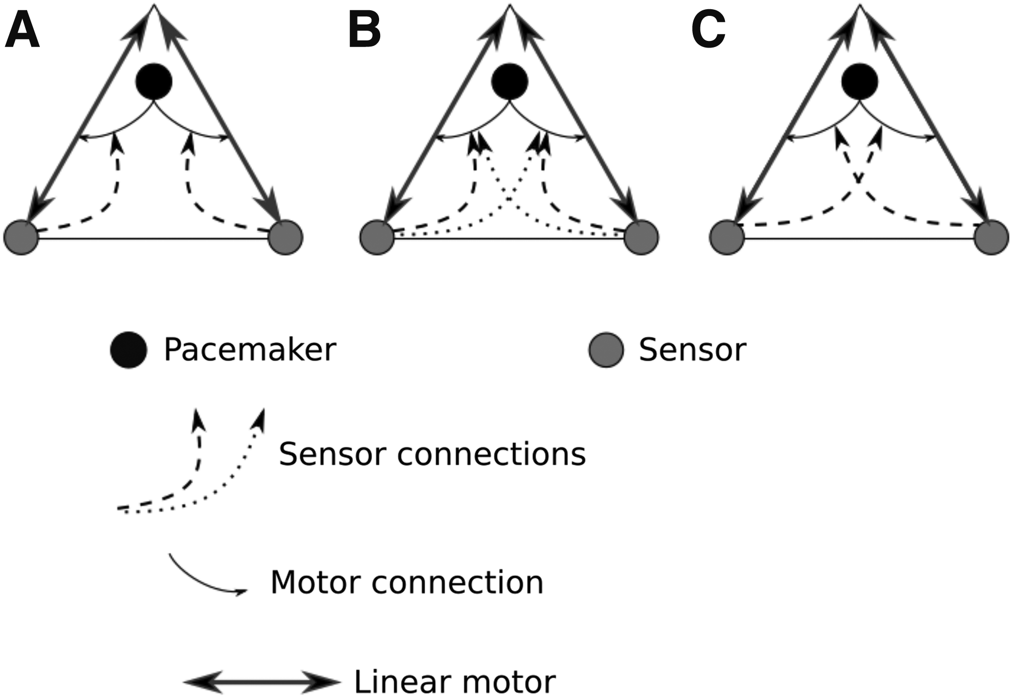
We found that with the particular parameters of our system, it was not necessary to apply feedback control to the joint lengths, as the actual lengths of the joints tracked the specified rest lengths with only a small lag. The pacemaker is a sinusoidal signal of fixed frequency, which is sent from a notional central circuit to both motors. The amplitude and phase of the signal may both be modulated at each motor according to the sensor outputs. We implemented three different control arrangements, detailed below and referred to as Swimmers A, B, and C, and shown in Figure 6.

FIG. 6.

Swimmers (A–C), shown from left to right. A central pacemaker synchronizes the motion of the left and right actuated faces. The phases of oscillation are modulated by the output of the sensors, placed on the vertices of the back face. Direct connections led to positive taxis, as in Swimmer (A) and Swimmer (B), and crossed connections led to negative taxis, as in the case of Swimmer (C). Swimmer (B) has additional crossed connections from the sensors which control the amplitudes of oscillation. The connections which modulate phase are shown as dashed lines, and the connections which modulate amplitude are shown with dotted lines.

Swimmer A has a constant amplitude of oscillation, of magnitude 0.5 m. For this swimmer, the connections from sensors to motors are uncrossed, and the phases of oscillation are equal to the respective sensor outputs. When the phases of oscillation between the two sides diverge, the swimmer tends to turn, as detailed in Turning section. When the sensors are equally distanced from the source of the chemical gradient, the oscillations are synchronized and the swimmer will travel in a straight line. Similarly to Braitenberg's Vehicle 2b, using this controller the swimmer will not stop when it reaches the source of the chemical gradient, but will typically swim past it a short distance before looping back toward it again.

Swimmer B has the same steering mechanism as Swimmer A, but has an additional function to control the amplitude of oscillation, so that when it is close to the source of the chemical gradient it will expend little or no energy in continuing to swim. This function is a nonlinearity, which has little effect beyond short distances from the source of the chemical gradient, but will stop the swimmer's motion when it has reached the source. When the swimmer reaches a point close to the source of the chemical gradient it will tend to stay very close to it, with its body rotating in position, under momentum for part of the time and actuation for the rest, as one or both of its sensors passes in and out of the region in which the stimulus amplitude falls to zero.

As with Braitenberg's vehicles, the behavior of a swimmer can be switched from positive to negative chemotaxis by merely switching the sensor connections from straight to crossed. Swimmer C is the same as Swimmer A except that the connections which control the phase of actuation are now crossed, which causes the swimmer to turn and travel away from the source of the chemical gradient.

Although the general behavior is determined by the nature, crossed or uncrossed, of the connections between sensors and motors controlling the phase of oscillation, the same is not true for the functions controlling amplitude. As long as the amplitude of oscillation decreases as the distance from the source of the chemical gradient decreases, the behavior of a swimmer is qualitatively unchanged by crossing or uncrossing the relevant connections.

For all triangular swimmers, the underlying motor functions are: \documentclass{aastex}\usepackage{amsbsy}\usepackage{amsfonts}\usepackage{amssymb}\usepackage{bm}\usepackage{mathrsfs}\usepackage{pifont}\usepackage{stmaryrd}\usepackage{textcomp}\usepackage{portland, xspace}\usepackage{amsmath, amsxtra}\usepackage{upgreek}\pagestyle{empty}\DeclareMathSizes{10}{9}{7}{6}\begin{document} \begin{align*} { \rm{restlengt}}{{ \rm{h}}_L} = { \rm{baselength}} + {A_L} + { \rm{sin}} ( 90t + { \phi _L} ) \tag{4} \end{align*} \end{document} \documentclass{aastex}\usepackage{amsbsy}\usepackage{amsfonts}\usepackage{amssymb}\usepackage{bm}\usepackage{mathrsfs}\usepackage{pifont}\usepackage{stmaryrd}\usepackage{textcomp}\usepackage{portland, xspace}\usepackage{amsmath, amsxtra}\usepackage{upgreek}\pagestyle{empty}\DeclareMathSizes{10}{9}{7}{6}\begin{document} \begin{align*} { \rm{restlengt}}{{ \rm{h}}_R} = { \rm{baselength}} + {A_R} + { \rm{sin}} ( 90t + { \phi _R} ) \tag{5} \end{align*} \end{document}

where angles are expressed in degrees. For Swimmers A and C, the amplitude of oscillation is a constant value: \documentclass{aastex}\usepackage{amsbsy}\usepackage{amsfonts}\usepackage{amssymb}\usepackage{bm}\usepackage{mathrsfs}\usepackage{pifont}\usepackage{stmaryrd}\usepackage{textcomp}\usepackage{portland, xspace}\usepackage{amsmath, amsxtra}\usepackage{upgreek}\pagestyle{empty}\DeclareMathSizes{10}{9}{7}{6}\begin{document} \begin{align*} {A_L} = {A_R} = 0.5 \tag{6} \end{align*} \end{document}

whereas for Swimmer B the amplitudes of oscillation are nonlinear functions of the sensor outputs: \documentclass{aastex}\usepackage{amsbsy}\usepackage{amsfonts}\usepackage{amssymb}\usepackage{bm}\usepackage{mathrsfs}\usepackage{pifont}\usepackage{stmaryrd}\usepackage{textcomp}\usepackage{portland, xspace}\usepackage{amsmath, amsxtra}\usepackage{upgreek}\pagestyle{empty}\DeclareMathSizes{10}{9}{7}{6}\begin{document} \begin{align*} { A_L } = \begin{cases} \begin{matrix} { 0.5 - \displaystyle \frac { 1 } { { \displaystyle { \rm { sensor } } _R^2 } } , } & { { \rm { if } } \; { \rm { senso } } { { \rm { r } } _R } \ge \sqrt 2 } \\ { 0 , } & { { \rm { otherwise } } } \\ \end{matrix} \end{cases}\tag { 7 } \end{align*} \end{document} \documentclass{aastex}\usepackage{amsbsy}\usepackage{amsfonts}\usepackage{amssymb}\usepackage{bm}\usepackage{mathrsfs}\usepackage{pifont}\usepackage{stmaryrd}\usepackage{textcomp}\usepackage{portland, xspace}\usepackage{amsmath, amsxtra}\usepackage{upgreek}\pagestyle{empty}\DeclareMathSizes{10}{9}{7}{6}\begin{document} \begin{align*} { A_R } = \begin{cases} \begin{matrix} { 0.5 - \displaystyle \frac { 1 } { { { \rm { sensor } } _L^2 } } , } & { { \rm { if } } \; { \rm { senso } } { { \rm { r } } _L } \ge \sqrt 2 } \\ { 0 , } & { { \rm { otherwise } } } \\ \end{matrix} \end{cases} \tag { 8 } \end{align*} \end{document}

For Swimmers A and B, the phases of oscillation are equal to the sensor outputs: \documentclass{aastex}\usepackage{amsbsy}\usepackage{amsfonts}\usepackage{amssymb}\usepackage{bm}\usepackage{mathrsfs}\usepackage{pifont}\usepackage{stmaryrd}\usepackage{textcomp}\usepackage{portland, xspace}\usepackage{amsmath, amsxtra}\usepackage{upgreek}\pagestyle{empty}\DeclareMathSizes{10}{9}{7}{6}\begin{document} \begin{align*} { \phi _L} = { \rm{senso}}{{ \rm{r}}_L} \tag{9} \end{align*} \end{document} \documentclass{aastex}\usepackage{amsbsy}\usepackage{amsfonts}\usepackage{amssymb}\usepackage{bm}\usepackage{mathrsfs}\usepackage{pifont}\usepackage{stmaryrd}\usepackage{textcomp}\usepackage{portland, xspace}\usepackage{amsmath, amsxtra}\usepackage{upgreek}\pagestyle{empty}\DeclareMathSizes{10}{9}{7}{6}\begin{document} \begin{align*} { \phi _R} = { \rm{senso}}{{ \rm{r}}_R} \tag{10} \end{align*} \end{document}

whereas for Swimmer C, the same is true but the connections are crossed: \documentclass{aastex}\usepackage{amsbsy}\usepackage{amsfonts}\usepackage{amssymb}\usepackage{bm}\usepackage{mathrsfs}\usepackage{pifont}\usepackage{stmaryrd}\usepackage{textcomp}\usepackage{portland, xspace}\usepackage{amsmath, amsxtra}\usepackage{upgreek}\pagestyle{empty}\DeclareMathSizes{10}{9}{7}{6}\begin{document} \begin{align*} { \phi _L} = { \rm{senso}}{{ \rm{r}}_R} \tag{11} \end{align*} \end{document} \documentclass{aastex}\usepackage{amsbsy}\usepackage{amsfonts}\usepackage{amssymb}\usepackage{bm}\usepackage{mathrsfs}\usepackage{pifont}\usepackage{stmaryrd}\usepackage{textcomp}\usepackage{portland, xspace}\usepackage{amsmath, amsxtra}\usepackage{upgreek}\pagestyle{empty}\DeclareMathSizes{10}{9}{7}{6}\begin{document} \begin{align*} { \phi _R} = { \rm{senso}}{{ \rm{r}}_L} \tag{12} \end{align*} \end{document}

Jet-propelled swimmer body plan

The body of the jet-propelled swimmer (Fig. 7) is principally composed of three rigid bodies shaped as slender isosceles triangles, connected to each other at the apices by revolute joints. The triangular bodies are symmetrically arranged about the swimmer's long axis, such that the spaces between them form left and right chambers, both open to water at the back. The triangles have long side length of 3 m, are ∼0.3 m wide at the base, and each have a mass of ∼0.47 kg. Small circular rigid bodies are attached with revolute joints at all of the vertices of the triangles, for convenience in calculating and applying drag forces, and for potential attachment of sensors and motors. These bodies have diameter of 0.05 m and density of 0.01 kg/m², such that their mass is negligible.

FIG. 7.

The body of the jet-propelled swimmer. The swimmer's body is principally composed of three rigid-body triangles, attached to each other with revolute joints. Small and almost massless circular bodies are attached to all triangle vertices for compatibility with methods of applying drag and attaching motors and sensors which were previously developed for the triangular swimmer. This swimmer is actuated by driving the revolute joints, seen at the top of this figure, so that the chambers open and close.

Jet-propelled swimmer controllers

The jet-propelled swimmer's chambers are opened and closed by actuating the revolute joints at the triangles' apices. At rest, the angular spacing between the triangular rigid bodies, which we denote \documentclass{aastex}\usepackage{amsbsy}\usepackage{amsfonts}\usepackage{amssymb}\usepackage{bm}\usepackage{mathrsfs}\usepackage{pifont}\usepackage{stmaryrd}\usepackage{textcomp}\usepackage{portland, xspace}\usepackage{amsmath, amsxtra}\usepackage{upgreek}\pagestyle{empty}\DeclareMathSizes{10}{9}{7}{6}\begin{document} $${ \alpha _r}$$ \end{document} , is \documentclass{aastex}\usepackage{amsbsy}\usepackage{amsfonts}\usepackage{amssymb}\usepackage{bm}\usepackage{mathrsfs}\usepackage{pifont}\usepackage{stmaryrd}\usepackage{textcomp}\usepackage{portland, xspace}\usepackage{amsmath, amsxtra}\usepackage{upgreek}\pagestyle{empty}\DeclareMathSizes{10}{9}{7}{6}\begin{document} $$ \frac { \pi } { { 12 } } $$ \end{document} . The function for calculating the reference angles of the chambers is \documentclass{aastex}\usepackage{amsbsy}\usepackage{amsfonts}\usepackage{amssymb}\usepackage{bm}\usepackage{mathrsfs}\usepackage{pifont}\usepackage{stmaryrd}\usepackage{textcomp}\usepackage{portland, xspace}\usepackage{amsmath, amsxtra}\usepackage{upgreek}\pagestyle{empty}\DeclareMathSizes{10}{9}{7}{6}\begin{document} \begin{align*} \alpha = 0.9 \cdot { \alpha _r} \cdot { \rm{sin}} ( 45t ) \tag{13} \end{align*} \end{document}

For this swimmer, the reaction forces from the surrounding and compressed fluids vary significantly over an actuation cycle, so we used a proportional-integral speed controller to ensure that the actual angle tracked the reference value. For straight line travel, both chambers are actuated identically (Fig. 8). For steering, the swimmer may be turned toward the left or right (Fig. 9) as it travels by actuating only one of its chambers. We have not implemented a closed loop behavior controller for this swimmer, as we did for taxis with the triangular swimmer.

FIG. 8.

The jet-propelled swimmer is pushed forward by the pressure created when it closes its chambers. It can be made to swim straight by activating both chambers equally. As can be seen by the trail drawn behind the swimmer to indicate its trajectory, it can be gradually pushed off course by irregularities in the arrangement of the particles.

FIG. 9.

The jet-propelled swimmer can be made to turn by activating only one chamber. In this example, only the right-hand chamber is actuated, which causes a turn toward the left. The trails behind the swimmer, in white and gray, indicate the trajectories of the swimmer's central and nose points, respectively.

Results

In this section, we begin by evaluating the gains in performance made through the use of the particle cloud for our triangular swimmer. We then test the support of the particle cloud environment for both positive and negative chemotaxis behaviors from the triangular swimmer, and for one behavior perform a direct comparison of trajectories between the two particle-based environments. We note the shortcomings of the fluid drag environment, for both of our swimmer morphologies. Finally, with our jet-propelled swimmer we identify an issue with the current particle cloud implementation, which we are now working on solving.

Performance

We tested the performance of the particle-based models using the triangular swimmer. Simulations were run on a linux machine with an AMD FX-6300 six core CPU and 16 GB of RAM. liquidfun is not parallelized, and so the simulation runs on a single processor core. When collecting data for this article, a significant amount of data, amounting to almost 17 MB for each run, was saved to file, but this process ran on a second core and only increased the cost of simulation by around 10%.

When the particle cloud method is used and there is no animation displayed, 90 s of simulated time can be executed in ∼40 s. Memory usage is negligible, at ∼30 MB. When a square tank of particles is simulated, with side length of 20 m, the time taken for a run of the same simulated duration took ∼11 min. Therefore, in this case, the use of the particle cloud increases computational efficiency by a factor of 16.5.

It should be noted that when using the particle cloud method, for a given particle density, the cost of simulation is related only to the size of the swimmer. If the swimmer is scaled up, the number of particles required to envelop it will also rise, quadratically, as noted in Reduced Particle-Based Simulation (Particle Cloud) section. In contrast, the spatial extents of the swimmer's environment have no effect on the size of the particle cloud, and so can be increased arbitrarily. In fact, where the particle cloud was used, the swimmers were initialized within the same region enclosed in the tank scenario, but the walls were not included in the simulation, and so in some cases Swimmer C, which is averse to the gradient source, travelled far beyond the tank's notional extents (Fig. 12).

Triangular swimmer behavior

In this section, we compare the behavior of the triangular swimmer in the different environments.

In all of the particle-based environment runs, swimmers begin at a randomly generated orientation and location inside a square-shaped region centered on the source of the gradient, with side length of 16 m. The simulation is then run for 90 simulated seconds, but the swimmer is not actuated for the first 700 ms, to give the particle system time to stabilize. This stabilization period is required because the methods of increasing pressure by doubling the number of particles introduce high energy to the particle system, which is not initially balanced by even distribution.

The source of the chemical gradient is not modeled as a physical body, and so the swimmers cannot crash into it. All swimmers were simulated for 40 runs with the particle cloud. Swimmer B was also simulated for the same number of runs in the water tank for comparison. So that the three controllers and the two particle-based environments can be compared directly, we used the same set of initial positions and orientations for all sets of runs.

Swimmers A and B (Figs. 10 and 11) both successfully perform positive chemotaxis in the particle cloud environment. Their trajectories toward the source of the chemical gradient are the same in almost all cases, although they differ when very close to the source, where Swimmer B is designed to halt. Swimmer C (Fig. 12) successfully performs negative chemotaxis in the particle cloud environment, in some cases travelling far beyond the notional extents of the tank in its escape from the chemical gradient.

FIG. 10.

Trajectories of Swimmer A. Swimmer A, similar to Braitenberg's Vehicle 2b, swims toward the source of the gradient, but does not stop when it reaches it. However, given how sensitive it is to a difference between sensor outputs, nor does it travel far beyond the source. Instead, it tends to keep circling back. In this figure, and the following three, the source of the chemical gradient is at the origin, indicated by a small open circle, and the swimmer's central position over time is shown in the traces. The swimmer is started from random positions and orientations. Clear trends in the effect of water current on the motion of the swimmer can be seen, with many trajectories pulled toward paths parallel to the x- and y-axes, and the lines which pass through zero and divide the quadrants of the x- and y-axes.

FIG. 11.

Trajectories of Swimmer B. The behavior of this swimmer is very similar to that of Swimmer A, except at short distances from the source of the gradient, where Swimmer B will slow down and eventually stop. It can be seen that the controller is not infallible, with one run, where the swimmer started at coordinates close to [−1, 2.5], resulting in the swimmer circling the gradient source rather than approaching it.

FIG. 12.

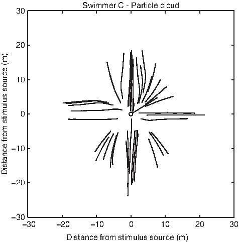
Trajectories of Swimmer C. Swimmer C performs negative phototaxis, swimming away from the source of the chemical gradient. As for Swimmers A and B, currents in the particle cloud often have a pronounced effect on the swimmer's trajectories.

In Figure 13 it can be seen that the behavior of Swimmer B in both particle-based environments is qualitatively similar and successful for almost all initial conditions. However, it is also apparent from Figures 10 –12 that the current method of injecting particles into the cloud is causing some bias in the swimmer's trajectory, and this is particularly evident for Swimmer B (Fig. 11), where the water currents tend to flow toward the source, at angles which divide the quadrants formed by the x- and y-axes.

FIG. 13.

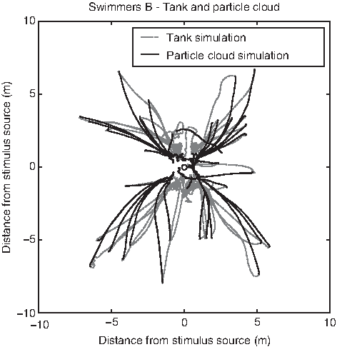
Trajectories of Swimmer B in both particle-based simulation variants. Apart from the one failed run in the particle cloud simulation, the behavioral differences are minor, with the swimmer's steering clearly affected by the different environments, but not enough to change the overall behavior.

In the drag-based fluid environment, Swimmers A, B, and C all turn to face in their respective correct directions but are incapable of travel. This is explained in Motion Analysis section.

Jet-propelled swimming

With the controller described in Jet-Propelled Swimmer Controllers section, the jet-propelled swimmer is incapable of travel in the drag fluid model environment, as the drag forces produced by the opening and closing motions of its chambers have equal and opposite effects and, therefore, cancel each other out. However, as drag is dependent upon the square of the velocity of the bodies, if the rate of closing is higher than the rate of opening then there will be a net force to push the swimmer forwards.

As already described in Jet-Propelled Swimmer Controllers section, this swimmer can be made to swim straight forward and to turn to either side in the tank environment. However, unlike the triangular swimmer, this swimmer does not function well in the particle cloud environment. Ultimately, this is due to the water pressure being lower in the cloud than it is in the tank. This results in the swimmer's chambers not always filling completely in the opening phase, meaning that a reduced and inconsistent amount of propulsive force is generated in the closing phase. For this swimmer, the problem is even worse for turning, where the momentum of the particle cloud can dominate the forces in the overall system and push the swimmer off the desired course.

To remedy this problem, we are currently developing an alternative to the particle cloud where a small tank (used to maintain pressure) moves around with the swimmer. To minimize the energy injected into the particle system by its motion, as the tank moves, particles are removed from the trailing edge of the system and replaced at the leading edge, effectively inducing a current with respect to the tank but not the swimmer (Fig. 16). Preliminary results suggest that this environment will support the behaviors of both of the swimmers that we used to test the particle cloud.

Motion analysis

In this section we perform some simple analysis of how our triangular swimmers are actually able to swim and to turn. Our objective here is not a complex or detailed analysis of the fluid dynamics involved in this, or of the swimming gaits, but rather to form a general overview of how this streamlined swimmer actually travels. We do this by breaking the sensorimotor loop and controlling the body of a swimmer first to simply swim forwards and then to rotate its body on the spot. In other words, we focus on the potential of the body–environment interactions here for the oscillating swimming style of the triangular swimmer, rather than the individual controllers that we have examined above.

Forward motion

To gain some insight into how the triangular swimmer moves, we first examined the case of swimming straight forwards. In this case, the two active sides of the body expand and contract synchronously. We will first deal with an observation from Triangular Swimmer Behavior section that the triangular swimmer cannot travel in the fluid drag model environment. This is to be expected. As we noted in Jet-Propelled Swimming section with reference to the jet-propelled swimmer, due to the sinusoidal pacemaker, the expanding and contracting phases of actuation mirror each other, meaning that the generated drag forces cancel out over time.

This swimmer can still be made to travel by breaking the symmetry of the control signal. For example, if the rate of the contraction is slower compared with expansion, then the drag forces from the two phases will not cancel out, due to the dependence of drag on the square of velocity.

We also found that this swimmer could not travel in the particle-filled tank if its frequency of actuation was too low. For comparison, we first ran the simulation with no fluid and found that under this condition the swimmer tends to slowly drift about its center, but does not change its position. When we restored the particles to the simulation, and lowered the frequency of the actuation cycle from 14.32 Hz to only 1 Hz, we found the same thing. From the observation that the swimmer only moves forwards in the presence of particles, we can conclude that in the energy exchange between swimmer and fluid, the successful swimmer wins and that some of the energy transferred from it to the surrounding fluid is returned to push it forwards.

In Figure 14, which shows the trajectories of particles and their velocities for a single actuation cycle of a swimmer at both tested frequencies, we see that at the lower frequency, the energy of particles around the swimmer's body is concentrated in much the same way relative to each of the swimmer's outer faces. This explains why the swimmer does not move in this case. In the case of the higher frequency, it is clear that energy is more concentrated behind the back face than it is to the sides, which explains how the swimmer is pushed forwards. While we do not consider the physics engine we use here to be completely realistic in all aspects, these contrasting effects appear to be broadly consistent with one aspect of swimming in biology, where, as noted by Purcell,²² reciprocal swimming motion like that of our swimmer is only effective at higher Reynolds numbers.

FIG. 14.

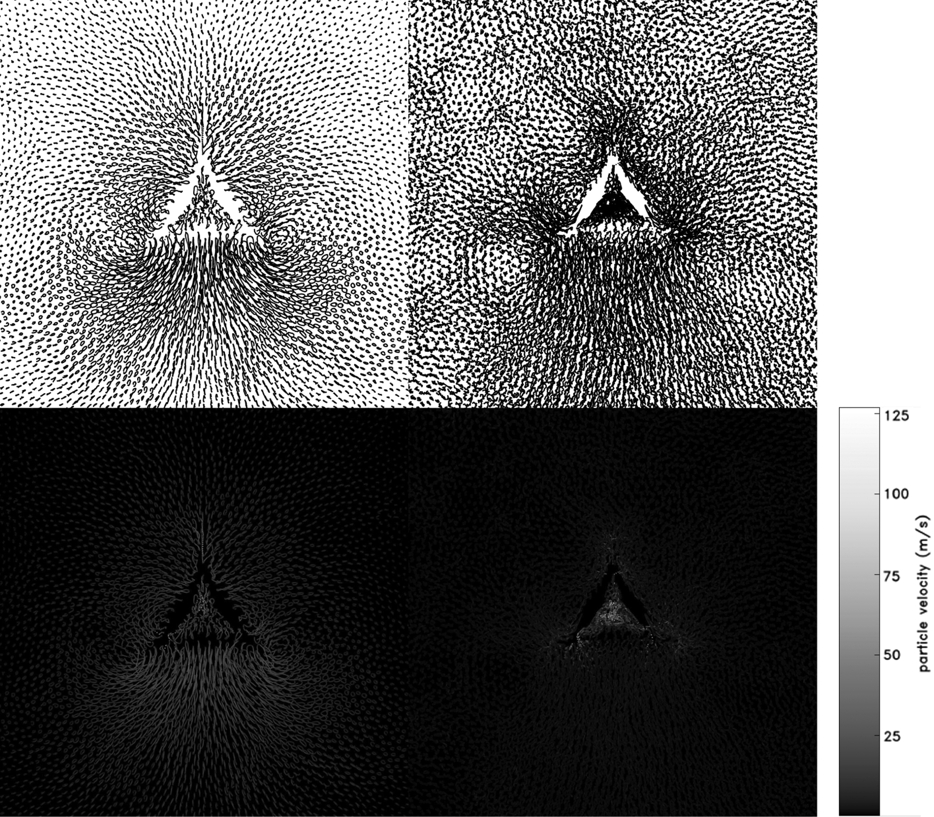
In this figure, the trajectories of particles are shown. In the top row, the traces show the positions of particles over time. In the bottom row, the same traces are shown, but color is used to illustrate the velocities of the particles. The left column shows a single cycle of oscillation of the swimmer's active joints, when the pacemaker is activating the joints at the normal frequency of 14.32 Hz. In the right-hand column, the same is shown for a swimmer with a pacemaker driving oscillation at the reduced frequency of 1 Hz. When we compare normal swimming to low frequency swimming, three points of contrast between the two stand out: First, the higher frequency oscillation imparts significantly more energy to surrounding particles than the lower frequency one, per oscillation cycle. Second, this higher energy leads to more structure in the motion of the particles in the higher frequency case. Third, the higher frequency case shows more energy behind the swimmer, on average, than on its sides, but the lower frequency case shows fairly uniform concentrations of energy on all sides of the swimmer. This last observation is consistent with the fact that the swimmer moves forwards with the 14.32 Hz pacemaker, but does not with the 1 Hz one. A final point to be made here is that in both cases, the effect of the swimmer's motion on the surrounding particles, and vice versa, falls to almost nil at ∼1.5 body lengths from its exterior faces. This led to the realization that it may be possible to minimize the number of particles in our simulation, as described in Reduced Particle-Based Simulation (Particle Cloud) section.

As well as this forwards motion that we designed for, we have discovered that the swimmer can also swim directly backwards in the tank environment, in the case that its two actuated sides oscillate exactly in antiphase.

Turning

While, for our triangular swimmers, travelling has a clear dependence on the surrounding fluid, we discovered that turning does not. Indeed, in the fluid drag based environment, we found that the swimmer could turn even though it could not travel.

We examined this case by setting the phase difference between the two oscillators to 90°. When the right oscillator leads, the swimmer turns left and vice versa. We set the swimmer to turn in three separate conditions: in the tank, in the particle cloud, and with no particles. In all cases, the motion was qualitatively the same, although the turning rate varied. The swimmer's turn is fastest in the tank condition, followed by the particle cloud, and finally the no particles condition. From this we conclude that although, as in traveling, the turning swimmer receives an energy rebate from its interaction with the surrounding fluid, which can increase its turning rate, the general turning motion results from the motion of the swimmer's own constituent bodies, when they are moved in the appropriate relative phases.

Figure 15 shows the turning motion of the swimmer for a single oscillation cycle during a left turn. The duration of the turn is split into four quarters, and for each quarter the initial profile of the swimmer is indicated with dashed lines and the final profile with solid lines. Quarters 2 and 4 are periods where both active sides contract and expand, respectively, and do not alter the swimmer's position or orientation considerably. Therefore it is apparent that the swimmer's turn over a single cycle is the net effect of quarters 1 and 3. As the two active sides oscillate with a 90° phase difference, the swimmer turns first one way and then the other, but the second turn is slightly larger than the first. This is because in quarter 3 the side lengths are shorter than in quarter 4, and so the motion of the nodes, which has the same magnitude in both cases, leads to a more pronounced effect in the second.

FIG. 15.

Turning. The four figures here show the motion of the swimmer over a single cycle of oscillation, split into four quarters. In each figure, the dashed lines show the swimmer's stance at the beginning of the quarter, and the solid lines show the stance at the end. The dotted lines connecting respective apices show the trajectories of the apex nodes during the quarter. The bold line in each profile connects the centroid of the triangle with the front apex. As the swimmer's mass is evenly distributed to nodes and scales on all sides, the centroid is also the swimmer's center of mass. Over a larger turn, the swimmer will tend to drift, but it can be seen here that for a single oscillation, the position of the center of mass is approximately constant.

In both cases (forward and turning motion) it is clear that it is the dynamical interactions between environment and the continually changing body morphology that are at the heart of the swimmer's motion.

Discussion

In evolutionary robotics, it is the norm to simulate robots for evaluation, from those which already exist to those which will exist if successful in simulation, to those which could feasibly exist although that is not planned. Virtual creatures lie at the end of the same scale, too abstract to be called robots, but sharing much common ground with them. For this reason, we can learn a lot about the problems facing robots, and solutions to them, from virtual creatures, in proportion to the similarity of their body–environment interactions with those encountered by real robots.

From the point of view of studying the importance to behavior of embodiment, and in particular morphological computation, we find the area of swimming soft bodies particularly appealing, due to the fact that in this case not only the body but also the substrate is soft, and even less constrained than the body of any animal or robot. The more types of body–environment interaction we can include in our simulations, the more we can learn about the dynamics of behavior in the given environment. To that end, we are developing computationally cheap methods of extending the range of simulated interactions between soft bodies and soft environments, using liquidfun particle-based physics as our test bed.

We implemented three models for interactions between swimmers and their environments. We used the fluid drag model of Sfakiotakis and Tsakiris¹¹ as a baseline for comparing our own particle-based models. Even though the fluid drag model is far cheaper to simulate than particle-based fluids, it is inferior in several regards. First, the fluid drag model is less realistic than the particle based fluid model. For example, it is well known that animals generate and exploit turbulent effects, which are not present in this model.^23,24 Although we have not yet demonstrated a virtual swimmer that clearly exploits turbulence, we have seen that turbulent effects appear in our fluids if enough energy is injected into the system. Second, from a control perspective, the fluid drag model environment may allow for less evolutionary pathways to efficient swimming than the particle-based one.

For example, for our swimmers to travel in the fluid drag model environment, they must not have controllers which drive expansion and contraction at the same rates, as in this case drag forces over a complete expand–contract cycle will cancel out. This constraint is not present in the particle-based environments.

Gains in realism in the particle-based environment can have a large computational cost, depending on the spatial dimensions and particle density of the simulated particle systems. When the particle cloud is used, the computational cost is not only dramatically reduced but also for a given swimmer is constant over environments of arbitrary size. We found that the current particle cloud implementation supports the behavior of our triangular swimmer, but not our jet-propelled one. The jet-propelled swimmer exposes a problem with maintaining pressure in the cloud, a problem which we are now working to solve.

In the case of the triangular swimmer, the same behaviors are supported by the particle cloud as are by the tank environment, but this is not because the cloud faithfully reproduces the tank dynamics, but rather because the dynamics are similar enough for the swimmer's closed sensorimotor loop to still be effective. We see this in Figure 13, where the swimmer's trajectories in the two environments initially diverge but still tend to reach the same area.

The triangular swimmer is the first example and test of our pseudo-soft technique for simulating controllable soft bodies using only rigid bodies and actuated and compliant joints, which interact in a realistic manner with particle-based fluids. This technique can be used to construct swimmers with arbitrary morphologies, with a skin of overlapping scales surrounding a triangulated structure where each edge can have unique dynamical properties and optionally be actuated. When we analyzed the travel produced by this swimmer's reciprocal swimming motion, we discovered an effect which Purcell²² described as occurring in biology, where travel is impossible at lower Reynolds numbers.

Having shown that particle-based fluids can make a good model for interactions between a swimmer's exterior and a surrounding fluid, we also tested a simple method for jet propulsion, where a swimmer is propelled forwards by the reaction force from water being expelled from its body. To make turning possible for this swimmer, we gave it two symmetrically arranged chambers. While the triangular swimmer can be turned by adjusting the relative oscillation phases of its two sides, the jet-propelled swimmer is more easily controlled by varying the oscillation amplitude. As we can make this swimmer travel directly forwards, and to turn left and right, then we could also close the loop for behavior, as we did for the triangle swimmer, although due to its large turning circle, the jet-propelled swimmer is less maneuverable.

By combining particle-based fluids and pseudo-soft bodies using liquidfun physics, we have addressed a disparity between the level of modeling of bodies and fluids in previous virtual creature experiments. However, the computational cost of simulating large areas of fluid is prohibitive for artificial evolution, and so we have also developed a novel means of minimizing the number of particles involved. As aforementioned, the jet-propelled swimmer exposed an issue with maintaining sufficient pressure in the particle cloud, and so we are already developing the next iteration of this technique; preliminary results (Fig. 16) are very encouraging. We are also developing an evolutionary framework incorporating these methods and an approach to extend them to three-dimensional environments.

FIG. 16.

The next stage in development of the particle cloud. To maintain pressure, a small mobile tank follows the swimmer in this case. To minimize the energy injected into the particle system by its motion, as the tank moves, particles are removed from the trailing edge of the system and replaced at the leading edge, effectively inducing a current with respect to the tank but not the swimmer. To observe the dynamics of the particle system, the color of removed and replaced particles is changed periodically, that is, colored bands represent intervals of time rather than waves in the usual sense.

Footnotes

Acknowledgments

C.J. was funded by the University of Sussex through a graduate teaching assistantship and the Research Development Fund. A.P. and P.H. have received funding from the European Union's Seventh Framework Programme for research, technological development, and demonstration under grant agreement no. 308943. A.P. is also funded by EPSRC grant: EP/P006094/1. We thank the anonymous reviewers whose comments and advice were a great help in improving this article.

Author Disclosure Statement

No competing financial interests exist.

Supplementary Material

*

Code for reproducing these experiments will be made publicly available at the github repository

References

Nolfi

, Bongard

, Husbands

, et al. Evolutionary robotics (Springer Handbook of Robotics, Chapter 76, 2nd Edition) Siciliano

, Khatib

(Eds). Cham: Springer, 2016, pp. 2035–2068.

Pfeifer

, Iida

. Morphological computation: connecting body, brain and environment. Jpn Sci Mon, 2005; 58:48–54.

Pfeifer

, Bongard

. How the Body Shapes the Way We Think: A New View of Intelligence. Cambridge, MA: MIT Press, 2006.

Rieffel

, Knox

, Smith

, et al. Growing and evolving soft robots. Artif life, 2014; 20:143–162.

Bongard

JC.

Evolving soft robots. Soft Robot, 2016; 3:43–44.

Corucci

, Cheney

, Giorgio-Serchi

, et al. Evolving soft locomotion in aquatic and terrestrial environments: effects of material properties and environmental transitions. Soft Robot, 2018; 5:475–495.

Joachimczak

, Suzuki

, Arita

. Artificial metamorphosis: evolutionary design of transforming, soft-bodied robots. Artif Life, 2016; 22:271–298.

Hauser

, Ijspeert

, Füchslin

et al. Towards a theoretical foundation for morphological computation with compliant bodies. Biol Cybern, 2011; 105:355–370.

Jakobi

Half-baked, ad-hoc and noisy: minimal simulations for evolutionary robotics (Fourth European Conference on Artificial Life). Cambridge, MA: MIT Press, 1997, pp. 348–357.

10.

Sims

Evolving virtual creatures (Proceedings of the 21st Annual Conference on Computer Graphics and Interactive Techniques). New York, ACM, 1994, pp. 15–22.

11.

Sfakiotakis

, Tsakiris

. Simuun: a simulation environment for undulatory locomotion. Int J Model Simul, 2006; 26:350–358.

12.

Schramm

, Sendhoff

An animat's cell doctrine (ECAL 2011: Proceedings of the 11th European Conference on the Synthesis and Simulation of Living Systems), Paris, France, ECAL, 2011, pp. 739–746.

13.

Hiller

Digital materials: voxel design, rapid assembly, structural properties, and design methods. PhD Thesis, Cornell University. 2011.

14.

Hiller

, Lipson

. Dynamic simulation of soft multimaterial 3D-printed objects. Soft Robot, 2014; 1:88–101.

15.

Google. liquidfun. 2013. Available at: http://google.github.io/liquidfun/ (accessed January 18, 2019).

16.

Braitenberg

Vehicles: Experiments in Synthetic Psychology. Cambridge, MA: MIT Press, 1986.

17.

Terzopoulos

, Tu

, Grzeszczuk

. Artificial fishes: autonomous locomotion, perception, behavior, and learning in a simulated physical world. Artif Life, 1994; 1:327–351.

18.

Rieffel

, Valero-Cuevas

, Lipson

. Morphological communication: exploiting coupled dynamics in a complex mechanical structure to achieve locomotion. J R Soc Interface, 2010; 7:613–621.

19.

Caluwaerts

, D'Haene

, Verstraeten

, et al. Locomotion without a brain: physical reservoir computing in tensegrity structures. Artif Life, 2013; 19:35–66.

20.

Katsuki

, Greenspan

. Jellyfish nervous systems. Curr Biol, 2013; 23:R592–R594.

21.

Cheney

, Clune

, Lipson

Evolved Electrophysiological Soft Robots (ARTIFICIAL LIFE 14: Proceedings of the Fourteenth Conference on the Synthesis and Simulation of Living Systems)

Sayama

, Rieffel

, Risi

, Doursat

, Lipson

. (Eds). Cambridge, MA: MIT Press, 2014, pp. 222–229.

22.

Purcell

EM.

Life at low Reynolds number. Am J Phys, 1977; 45:3–11.

23.

Gemmell

, Colin

, Costello

et al. Suction-based propulsion as a basis for efficient animal swimming. Nat Commun, 2015; 6:8790.

24.

Park

, Kim

, Lee

, et al. Dynamics of prolate jellyfish with a jet-based locomotion. J Fluids Struct, 2015; 57:331–343.

Supplementary Material

Please find the following supplemental material available below.

For Open Access articles published under a Creative Commons License, all supplemental material carries the same license as the article it is associated with.

For non-Open Access articles published, all supplemental material carries a non-exclusive license, and permission requests for re-use of supplemental material or any part of supplemental material shall be sent directly to the copyright owner as specified in the copyright notice associated with the article.

109.60 MB

54.94 MB

63.39 MB

28.61 MB

144.85 MB

0.03 MB

0.00 MB