A Geometrically Exact Model for Soft Continuum Robots: The Finite Element Deformation Space Formulation

Abstract

Mathematical modeling of soft robots is complicated by the description of the continuously deformable three-dimensional shape that they assume when subjected to external loads. In this article we present the deformation space formulation for soft robots dynamics, developed using a finite element approach. Starting from the Cosserat rod theory formulated on a Lie group, we derive a discrete model using a helicoidal shape function for the spatial discretization and a geometric scheme for the time integration of the robot shape configuration. The main motivation behind this work is the derivation of accurate and computational efficient models for soft robots. The model takes into account bending, torsion, shear, and axial deformations due to general external loading conditions. It is validated through analytic and experimental benchmark. The results demonstrate that the model matches experimental positions with errors <1% of the robot length. The computer implementation of the model results in SimSOFT, a dynamic simulation environment for design, analysis, and control of soft robots.

Introduction

Soft robots are autonomous systems with a continuously deformable mechanical structure, which provide them novel capabilities relative to traditional rigid robots. The configuration space of soft robots is (theoretically) infinite, meaning that, the robot tip can reach every point in its three-dimensional workspace with a (theoretically) infinite number of shape configurations.¹ Exploiting finite strain deformations, soft robots can adapt their shape to nonlinear paths, access difficult-to-reach remote environments, and squeeze through openings smaller than their nominal dimensions.² These features enable soft robots to perform delicate tasks in cluttered and/or unstructured environments, as well as to investigate novel grasping and manipulation possibilities. Furthermore, the compliance of their underlying material makes them ideal for applications that require a safer physical human–robot interaction.

As a matter of fact, soft continuum robots have proven their capabilities in several robotic fields, such as minimally invasive robotic surgery,³ robotic rehabilitation,^4,5 autonomous remote maintenance and inspection in industrial^6,7 and space⁸ environments, and physical human–robot interaction.⁹

Besides the interesting applications, fundamental topics in robotics need to be revised and expanded with novel principle and methods to provide a solid theoretical foundation on soft mechanisms. In this respect, over the past few years, significant advancements have been done in design and fabrication,^10–12 planning and control,^13–19 grasping and manipulation,^20–22 and robotic locomotion.^23–25 This article focuses on modeling aspects. The considered problem statement and related work are introduced next, leading to the overall contributions made.

Problem statement

Real-time model-based analysis, simulation, planning, and control of soft robotic manipulators are complicated by the lack of dynamic models that are at the same time accurate and computationally efficient. Therefore, our overall goal is to derive a soft robots dynamic formulation able to handle geometric nonlinearities, which is:

accurate, using a geometrically exact approach for large deformations;

computationally efficient, using a finite element spatial integration and a geometric time integration.

Review of relevant literature

Currently, the most adopted practice in the soft robotics community is to approximate the robot's shape as a series of mutually tangent circular arcs, which are described by only three parameters, namely the radius of curvature, angle of the arc, and bending plane. This is known as the constant curvature kinematic assumption.²⁶ This approximation has been verified experimentally in many continuum robots.^27–29 However, when extreme loading conditions lead to complicated robot's shape, variable curvature kinematic frameworks combined with elasticity theories for slender objects are preferable.³⁰

The widely used approach in the past years was the classical Bernoulli–Euler beam theory, which makes the assumption of small deflections. The planar large-deflection Bernoulli–Euler elastica theory and its analytical solution in terms of elliptic functions were used to describe the exact mechanics of planar robotic arms.³¹ Timoshenko beam models have also been investigated to include shear effects.³²

A promising approach for modeling soft continuum robots comes from the Cosserat rod theory and its particular case Kirchoff rod theory, which neglects shear and axial strains. This theory can be conveniently used to obtain general models of continuum robots.

Since the pioneering works of Simo and Vu–Quoc^33,34 on geometrically exact beam theory in finite strains, several nonlinear models have been derived in continuum mechanics.^35–39

Continuum models have been used for the first time in robotics by Chirikjian,⁴⁰ to approximate the shape of hyper-redundant or snake-like manipulators. Then, geometrically exact models based on Cosserat rod theory have been used for continuum manipulators. Boyer et al.⁴¹ introduced for the first time the idea of using the internal strains to compute the three–dimensional movements of a swimming eel–like robot.

Trivedi et al.⁴² developed a static model of the OctArm manipulator using Cosserat rod theory and a fiber-reinforced model of the air muscle actuators. Rucker et al.⁴³ for the first time modeled the static shape of an active cannula (a concentric tube robot) as a Cosserat rod under external loading. Afterward, they extended the theory to dynamic modeling of tendon-driven manipulator.⁴⁴ To numerically solve the dynamic equations, they used the Richtmyer's two-step variant of the Lax–Wendroff finite difference scheme implemented in a suite of MATLAB software written by Shampine.⁴⁵

The large-scale integrating European Project OCTOPUS has led to the manufacturing of a prototype arm inspired by the octopus vulgaris.⁴⁶ To model this robot, Renda et al. considered external dynamic loads in the Cosserat rod equations, derived using geometric notations. To numerically solve this model, they first involved an upwind finite difference method for hyperbolic equations, based on explicit time integration and a decentralized space differentiation.⁴⁷ More recently, they have proposed a dis-crete Cosserat approach involving piece–wise constant strains.^47–49 They have extended to the robotics community the approach of using piece–wise helical arcs for discretization of Cosserat rod models, until now used (beyond computational mechanics) only for computer graphics applications.^50,51 Despite their proven accuracy, these models are still computationally inefficient and, thus, difficult to use for real-time applications, when dynamics comes into play.⁴⁷ Furthermore, some of them are specifically derived for custom manipulators. In this paper we start from the idea of using deformations as degree–of–freedom for modeling chains of soft bodies.^40,47,51 Our purpose is to extend the recent advancements in Cosserat rod modeling of soft robots to a general full geometric framework, involving both geometric spatial and geometric temporal integration techniques, in a finite element fashion. This framework outperforms previous studies by reaching a compromise between accuracy and computational efficiency which is promising towards the development of model–based, real–time applications of soft robots.

Contributions

We model a soft robotic arm as the continuous assembly of cross sections moving upon a three-dimensional curve according to infinite rigid body transformations that are defined by distributed laws of internal deformations. This means that we do not consider warping effects and area change of the cross sections. The kinematic assumption of considering rigid cross sections allows to describe mathematically the soft arm in terms of the Lie group structure of rigid body motions, and to use the powerful techniques of modern differential geometry. Our model is geometrically exact since it makes no approximation on kinematic variables, thus it can reproduce the exact nonlinearity in the deformations due to bending, torsion, shear, and extension.

To the best of authors' knowledge, the use of a formalism combining screw theory, Lie groups and Lie algebras, Cosserat rod models, and the finite element method, for modeling geometrically nonlinear arms, is considered here for the first time in the soft robotics community.

The contributions of this work are as follows.

Lie group formulation suitable for soft robots dynamics using the Hamilton's variational principle of mechanics.

Spatial integration using helical shape functions for the finite element. This leads to a simple description of the forward and inverse kinematics of the soft arm, using the exponential and logarithmic mappings. The model is valid for straight and curved initial configuration of the arm. Furthermore, a geometrical interpretation of the reference curve that interpolates the soft arm is provided.

Derivation of a finite element soft geometric Jacobian, which relates the velocity of the arm with the time derivative of the deformations. The soft geometric Jacobian constitutes an essential tool to describe the statics, using the principle of virtual work, and the dynamics, derived from the weak form of the dynamic equilibrium equations of the continuum formulation. The proof of the kinetostatic duality and the derivation of a dynamic model with the same structure of the serial rigid manipulators are observed.

Geometric time integration using the implicit generalized α Lie group scheme, and the computer implementation that results in SimSOFT, a physics engine for soft robots.

Analytically integrable models for soft robots, including one cantilever soft arm in pure bending and one soft arm in planar rotation. Even if simple, analytic models are useful to guide the intuition for developing manageable mathematical models for more complex situations.

Experimental validation of the discrete model with the Princeton benchmark, which involves in-plane and out-of-plane motions where bending, torsion, and shear are coupled.

Examples of dynamic simulations of soft robots with different settings and in different scenarios.

Outline

The remainder of the article is organized as follows. Continuum Formulation section formulates the continuum model of Cosserat rods on a Lie group. The derivation of the finite element-based deformation space formulation is presented in The Deformation Space Formulation section, whereas the geometrical interpretation of the interpolated reference curve together with a dynamic example is presented in Geometrical Interpretation section. Special Cases section reports special examples that are analytically integrable. The experimental validation of the model is presented in Experimental Validation section. Some application scenarios are discussed in Application Scenarios section, with conclusions given in Conclusion section. Finally, in Appendices A1 and A2, the basic concepts and notations for Lie groups are reported.

Continuum Formulation

Position field

The three-dimensional reference curve is parameterized by the material abscissa $α \in [0, L]$ . Figure 1 shows the geometric description of the curve in the initial and current configurations. We indicate the position vector of a point of the curve with $u (α)$ . The unit tangent vector $t (α)$ , the unit normal $n (α)$ , and the unit binormal $b (α)$ to the curve constitute a local triad on the reference curve. Thus, a rotation matrix $R \in S O (3)$ to represent the orientation can be introduced as

FIG. 1.

Geometric description of the reference curve for the continuum arm.

R (α) = [t (α) n (α) b (α)]

(1)

Hence, the position field, which describes the configuration of the continuum arm, is represented by the mapping $α \in ℝ \mapsto H (α) = ℋ (R (α), u (α)) \in S E (3)$ (2)

Deformation field

The deformation field is obtained by taking the space derivatives of the position field. We introduce an element $\tilde{f} (α) \in s e$ (3) representing the deformation measures as $H^{'} (α) = H (α) \tilde{f} (α) .,$ (3)

where ${(\cdot)}^{'}$ denotes the space derivative with respect to $α$ . The deformation measures are identified from the initial configuration as $f (α) = f^{0} (α) + ε (α)$ (4)

where $f^{0}$ is the initial deformation vector and $ε (α) =[γ {(α)}^{T} κ (α)^{T}]^{T}$ is the 6 $\times$ 1 strain vector that includes the classical position part and the rotation part of the deformations. Note that Eq. (3) accounts for soft arms of generic initial configurations (not necessarily straight).

Velocity field

The velocity field is obtained by taking the time derivatives of the position field. We can introduce the velocity variables as an element $\tilde{η} (α) \in s e$ (3), which is associated with the 6 × 1 axial vector $η (α) = {[ν {(α)}^{T} ω {(α)}^{T}]}^{T}$ that includes the linear and angular velocities. Hence, the derivative of Eq. (2) with respect to time yields $\dot{H} (α) = H (α) \tilde{η} (α),$ (5)

which constitutes the velocity field along the continuum arm.

Compatibility equations

Compatibility conditions for finite strains in continuum mechanics are formulated such that the body is left without unphysical gaps or overlaps after a deformation. This translates into formulating compatibility conditions between the strain and the velocity of a continuum body. Since two different derivatives are involved to define the strain and the velocity, respectively, the space and time derivatives, the commutativity of the cross derivatives must hold from Eq. (120). Hence, this condition is used to formulate the compatibility equations as $η^{'} - \overset{έ}{ε} = \hat{η} ε .$ (6)

Notice that similar compatibility equations, according to Eq. (119), can be formulated as ${\tilde{η}}^{'} - \dot{\tilde{ε}} = [\tilde{η}, \tilde{ε}]$ , where $[\cdot, \cdot]$ indicates the Lie bracket operator.

Strain energy

The internal strain energy of the continuum arm is defined as $ν_{i n t} = \frac{1}{2} \int_{L} ε^{T} σ d α,$ (7)

where $σ = [n (α)^{T} m (α)^{T}]^{T}$ is the vector of the stress resultants over the cross section of the arm, and $n$ and $m$ are the $3 \times 1$ resulting force and resulting moment vectors. In particular, n₁ is the force along the reference curve, whereas n₂ and n₃ are the shear forces along the cross section axes. Indeed, m₁ is the torsion moment about the reference curve, whereas m₂ and m₃ are the bending moments about the cross section axes.

The internal force $σ$ and the mechanical strains $ε$ can be related through the material constitutive law. Linear constitutive equations for an isotropic hyperelastic material were chosen both for the elastic and the viscous members, and no bulge effects were considered. This simplified approach suits for robotics applications, where the objective is to describe the global dynamics and the geometric properties of the system, rather than a detailed material behavior. The simplest viscoelastic constitutive model is the Kelvin–Voigt model,⁴⁹ which simply adds viscous linear contributions, proportional to the rate of the strains, to the elastic contributions, as $σ = K ε + ϒ \dot{ε},$ (8)

where $K$ and $ϒ$ are, respectively, the $6 \times 6$ stiffness matrix and the $6 \times 6$ viscosity matrix equal to $K = [\begin{matrix} K_{u u} & K_{u ω} \\ S Y M & K_{ω ω} \end{matrix}] a n d ϒ = [\begin{matrix} ϒ_{u u} & ϒ_{u ω} \\ S Y M & ϒ_{ω ω} \end{matrix}] .$ (9)

In general, these matrices are not diagonal. But, in the case of an initially straight configuration of the soft arm, they become diagonal when the reference curve is chosen to be the neutral axis of the arm, and $n$ and $b$ are chosen to be the principal axes of the cross sections. In such case, $K_{u u} = d i a g (E A, G A_{2}, G A_{3})$ contains the axial and shear stiffnesses and $K_{ω ω} = d i a g (G J, E I_{2}, E I_{3})$ contains the torsional and bending stiffnesses, E and $G \in ℛ$ being the Young modulus and the shear modulus. For an isotropic material, it holds $G = E ∕ 2 (1 + ν)$ , where $ν \in ℛ$ is Poisson's ratio. Similarly, $ϒ_{u u} = d i a g (3 A, A, A) μ$ is the linear part of the viscosity tensor and $ϒ_{ω ω} = d i a g (J_{1}, J_{2}, J_{3})$ is the rotational part, for an incompressible material, where $μ \in ℛ$ is the shear viscosity.

Using Eq. (8), Eq. (7) becomes $ν_{i n t} = \frac{1}{2} \int_{L} ε^{T} K ε d α + \frac{1}{2} \int_{L} ε^{T} ϒ \dot{ε} d α,$ (10)

where the first term on the right-hand side recalls the well-known structure of the internal energy for a linear elastic material expressed as a quadratic form in $ε$ .

Static equilibrium equations

According to the principle of virtual work, the manipulator is in static equilibrium if and only if $δ (ν_{i n t}) = δ (ν_{e x t}),$ (11)

where $δ (ν_{e x t})$ is the virtual work done by the external forces. The variation of the expression of the internal energy, Eq. (7), reads $δ (ν_{i n t}) = \int_{L} δ (ε)^{T} σ d α,$ (12)

where, recalling the commutativity of the Lie derivatives in Eq. (120), the variation of the strains is expressed as $δ (ε) = δ (f) = {(δ h)}^{'} + \hat{f} δ h,$ (13)

in which we used $δ (H (α)) = H (α) \tilde{δ h} (α)$ . Inserting Eq. (13) into Eq. (12) and integrating by parts yield $δ (ν_{i n t}) = [δ h^{T} σ] |_{0}^{L} - \int_{L} δ h^{T} (σ^{'} - {\hat{f}}^{T} σ) d α,$ (14)

where the first term on the right-hand side is interpreted as a boundary condition.

In general, the virtual work done by the external forces can be expressed as $δ (V_{e x t}) = + δ h {(0)}^{T} g_{e x t} (0) - δ h {(L)}^{T} g_{e x t} (L) - \int_{L} δ h^{T} g_{e x t} d α,$ (15)

where $g_{e x t} (α) = [g_{e x t, u}^{T} g_{e x t, ω}^{T}]$ contain the resulting forces and moments over the cross sections due to external loading, expressed in the local frames attached to the cross sections.

Finally, the weak form of the static equilibrium equations is obtained by inserting Eqs. (15) and (14) into Eq. (11), which yields $[δ h^{T} (σ - g_{e x t})] |_{0}^{L} - \int_{L} δ h^{T} (σ' - {\hat{f}}^{T} σ - g_{e x t}) d α = 0.$ (16)

Indeed, the strong form reads $σ^{'} - {\hat{f}}^{T} σ = g_{e x t} .$ (17)

Kinetic energy

The kinetic energy of the continuum arm is defined by $K = \frac{1}{2} \int_{L} η^{T} M η d α,$ (18)

where M is the constant $6 \times 6$ inertia matrix, which contains the usual mass and rotation inertia properties of the cross sections as $M = [\begin{matrix} ρ A I_{3 \times 3} & J_{I}^{T} \\ J_{I} & J_{I I} \end{matrix}],$ (19)

in which $J_{I}$ and $J_{I I}$ are the first and second moment of inertia of the cross sections computed in the local axes of the arm, $ρ$ is the density, and A is the cross section area. In the general case, $M$ is not diagonal. Indeed, if the reference curve is defined such that $J_{I} = 0_{3 \times 3}$ , and if the normal and the binormal to the reference curve are the principal axes of the cross sections such that $J_{I I}$ is diagonal, then $M$ is a diagonal matrix. Since the cross sections are assumed to be undeformable, $M$ is defined from the initial configuration of the continuum arm and it does not depend on its motion or deformation.

Dynamic equilibrium equations

The dynamic equilibrium equations of the continuum arm can be obtained from Hamilton's principle, which states that the action integral over the time interval $[t_{0}, t_{1}]$ is stationary provided that the initial and final configurations are fixed, that is, $\int_{t_{0}}^{t_{1}} (δ (K) - δ (V_{i n t}^{}) + δ (V_{e x t}^{})) d t = 0 .$ (20)

where the variations are fixed at t₀ and t₁. In Eq. (20), $K$ denotes the kinetic energy, whereas $ν_{i n t}$ and $ν_{e x t}$ denote, respectively, the potential energy due to the internal and external forces. The variations of the strain energy and the external forces are the same as the static case. The variation of the kinetic energy in Eq. (18) reads $δ (K) = \int_{L} δ {(η)}^{T} M η d α .$ (21)

By recalling the commutativity of the Lie derivatives in Eq. (120), the variation of the velocity in terms of the variation of the configuration variables is expressed as $δ (η) = (δ \dot{h}) + \hat{η} δ h$ (22)

Inserting Eq. (22) into Eq. (21) and integrating by parts yield $\int_{t_{0}}^{t_{1}} δ (K) d t = {[\int_{L} δ h^{T} M η d α]}_{_{t_{0}}}^{t_{1}} - \int_{t_{0}}^{t_{1}} \int_{L} δ h^{T} (M \dot{η} - {\hat{η}}^{T} M η) d α d t$ (23)

Since the variations are fixed, the first term on the right hand side vanishes. Finally, by combining Eq. (23) and Eq. (16), Hamilton's principle in Eq. (20) yields the following weak form of the dynamic equilibrium equations $[δ h^{T} (σ - g_{e x t})] |_{0}^{L} - \int_{L} δ h^{T} (- M \dot{\dot{η} +} \hat{η} M η + σ' - {\hat{f}}^{T} σ {+ g}_{e x t}) d α = 0.$ (24)

Indeed, the strong form of the dynamic equations of the continuum arm reads $M \dot{η} - {\hat{η}}^{T} M η - σ^{'} + {\hat{f}}^{T} η σ + g_{e x t} = 0 .$ (25)

The Finite Element Deformation Space Formulation

In this section, we derive the deformation space formulation for kinematics, statics, and dynamics of soft robots using a finite element approach.

The finite element approach

The finite element method is a spatial discretization technique for solving partial differential equations [as Eq. (25)]. This method schematically models a generic mechanical system with a finite set of nodes which are interpolated by proper shape functions. Therefore, the same approach can be used to simulate both serial and/or parallel chains of soft bodies. This could be of great advantage for the soft robotics community, due to the recent growing interests also in parallel continuum robots. Indeed, these systems might improve robot–assisted surgery by providing instruments easy to miniaturize, and which can achieve multi degrees–of–freedom motion in confined spaces.^52,53 In the following we describe the dynamics of a single finite element which is used to simulate the behavior of a single–segment soft manipulator. This finite element is composed by two nodes which are interpolated by a helical shape function, and its behavior is described by the internal deformations. Multi–segments (even branched) soft manipulators, are simulated by considering a mesh composed by n finite elements, being n the number of segments of the soft arm.

Forward kinematics

The forward kinematics gives the mapping from the deformation field to the $S E (3)$ field of the soft arm. The objective is to find a suitable function that can be used to reconstruct the shape of the manipulator starting from the internal deformations. In this work, we propose to use a helical shape function⁵⁰ as $H (α) = H_{A} H_{A 0} e x p_{S E (3)} (α f),$ (26)

where $H_{A} = ℋ (R_{A}, u_{A})$ is the nodal frame A located at $α = 0$ ; $H_{A 0} = ℋ (R_{A 0}, 0)$ is a constant frame that accounts for the initial orientation of the cross section, allowing the description of initially curved arms; $f$ is the vector of deformations as in Eq. (4); $e x p_{S E (3)} (\cdot)$ is the exponential mapping on $S E (3)$ , which is given by Eq. (123).

The forward kinematics mapping in Eq. (26) has an analytic interpretation. As a matter of fact, Eq. (26) is the closed-form solution of Eq. (3), when $f$ does not depend on $α$ . Therefore, using helical shape functions, the deformation space formulation forces the deformations to be constant along the arm. At any instant t, considering the deformation field $f (α)$ (and thus, the strain field $ε (α)$ ) constant along the arm, we can replace the continuous field with a six-dimensional twist vector $f$ , which will play for the soft arm the same role of the joint vector for the traditional rigid arm.⁴⁷ Indeed, we can see a constant deformation soft arm, where all the six components of deformations are considered constant, as a six degrees-of-freedom traditional rigid robotic manipulator.

Let us introduce the relative configuration vector $d =[d_{u}^{T} d_{ω}^{T}]^{T}$ defined as $d = f L$ . Hence, Eq. (26) becomes $H (α) = H_{A} H_{A 0} {exp}_{S E (3)} (\frac{α}{L} d) .$ (27)

Eq. (27) represents a formula for the interpolation of frames, which are elements belonging to SE(3), that is, a noncommutative and nonlinear space. In geometric terms, this equation can be interpreted as, starting from the nodal frame, $H_{A} = H (α = 0)$ , the nodal frame $H_{B} = H (α = L)$ is approached by moving along the frame transformation implied by the projection on the group of the relative configuration vector d d. The use of the exponential map introduces a local parameterization that allows the description of the reference curve between the two nodes A and B with an element belonging to a linear space, namely the Lie algebra $s e$ (3). The discretization process is illustrated in Figure 2.

FIG. 2.

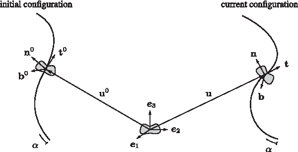
Soft arm in its initial and current configuration.

Eq. (27) represents the forward kinematics for soft robots using the exponential mapping.

Inverse kinematics

The inverse kinematics gives the mapping from the position and orientation fields to the deformation field of the soft arm. By considering the inversion of the exponential function in Eq. (27), we have $d = l o g_{S E (3)} (H_{A 0}^{- 1} H_{A}^{- 1} H_{B} H_{B 0}),$ (28)

where $l o g_{S E (3)} (\cdot)$ is the logarithmic mapping given in Eq. (126), and, in the same manner as $H_{A 0}$ , $H_{B 0} = ℋ (R_{B 0}, 0)$ is a constant frame that accounts for the initial orientation of the cross section of the end node. Using Eq. (4), the strain field reads $ε = \frac{d - d_{0}}{L},$ (29)

where $d^{0}$ is the relative configuration vector in the initial configuration, which is given by $d^{0} = [\begin{matrix} d_{u}^{0} \\ d_{ω}^{0} \end{matrix}] = [\begin{matrix} T_{S O (3)}^{- T} (d_{ω}^{0}) R_{A 0}^{T} (u_{B}^{0} - u_{A}^{0}) \\ l o g_{S O (3)} (R_{A 0}^{T} R_{B 0}) \end{matrix}],$ (30)

where $l o g_{S O (3)} (\cdot)$ is the logatithmic map on SO(3) given in Eq. (127), and $T_{S O (3)}^{- 1} (\cdot)$ is the inverse of the tangent operator on SO(3) given in Eq. (133).

Differential kinematics

The differential kinematics aims at finding a mapping between the velocity vector along the arm and the time derivatives of the state of the soft manipulator, namely the internal deformation vector.

We start from computing the time derivative of Eq. (27), which can be conveniently achieved using the following two expressions: $\dot{H} (α) = H (α) \tilde{η} (α) .$ (31) $\begin{matrix} \dot{H} (α) = & {\dot{H}}_{A} H_{A 0} {exp}_{S E (3)} (\frac{α}{L} = d) + \dots \\ + H_{A} H_{A 0} D ({exp}_{S E (3)} (\frac{α}{L} d)) \frac{α}{L} \dot{d} \end{matrix} .$ (32)

In particular, Eq. (31) has been obtained according to the definition of the left invariant vector field for Lie derivatives in Eq. (113), whereas Eq. (32) has been obtained according to the definition of derivatives in general, $D (e x p_{S E (3)} (\cdot))$ being the directional derivative of the exponential mapping in the direction of $d$ . By inserting Eq. (27) into Eq. (31) and by considering that ${\dot{H}}_{A}$ in Eq. (32) can be expressed as $H_{A} {\tilde{η}}_{A}$ , the equivalence of Eqs. (31)–(32) yields $\begin{matrix} H_{A} H_{A 0} {exp}_{S E (3)} (\frac{α}{L} d) \tilde{η} (α) = \dots \\ \dots H_{A} {\tilde{η}}_{A} H_{A 0} {exp}_{S E (3)} (\frac{α}{L} d) + \dots \\ \dots + H_{A} H_{A 0} D ({exp}_{S E (3)} (\frac{α}{L} d)) \frac{α}{L} \dot{d} . \end{matrix}$ (33)

Premultiplication of Eq. (33) with the quantity ${(H_{A} H_{A 0} e x p_{S E (3)} (\frac{α}{L} d))}^{- 1}$ leads to $\begin{matrix} \tilde{η} (α) = {exp}_{S E (3)} {(\frac{α}{L} d)}^{- 1} H_{A 0}^{- 1} {\tilde{η}}_{A} H_{A 0} {exp}_{S E (3)} (\frac{α}{L} d) + \dots \\ \dots + {exp}_{S E (3)} {(\frac{α}{L} d)}^{- 1} D ({exp}_{S E (3)} (\frac{α}{L} d)) \frac{α}{L} \dot{d} \end{matrix} .$ (34)

By considering the adjoint representation of a Lie algebra element in Eq. (117), we obtain $\begin{matrix} \tilde{η} (α) = {A d}_{exp}_{S E (3)} {(\frac{α}{L} d)}^{- 1} H_{A 0}^{- 1} {\tilde{η}}_{A} + \dots \\ \dots + {exp}_{S E (3)} {(\frac{α}{L} d)}^{- 1} D ({exp}_{S E (3)} (\frac{α}{L} d)) \frac{α}{L} \dot{d} \end{matrix} .$ (35)

Eq. (35) can be written in terms of the axial vectors by using the tangent operator in Eq. (129) as $η (α) = {A d}_{e x p_{S E (3)}} {(\frac{α}{L} d)}^{- 1} H_{A 0}^{- 1} η_{A} + T_{S E (3)} (\frac{α}{L} d) \frac{α}{L} \dot{d} .$ (36)

Eq. (36) relates the velocity along the arm with the initial velocity and the time derivative of the deformations, since it holds $\dot{ε} = \dot{d}$ . To relate the velocity along the arm with the time derivative of the deformations, we need to write the initial velocity $η_{A}$ as function of $\dot{d}$ . From Eq. (27), a relationship between the initial frame and final frame is given as $H_{A} H_{A 0} = H_{B} H_{B 0} {exp}_{S E (3)} (- d)$ (37)

\Leftrightarrow A d_{H_{A 0}^{- 1}} η_{A} = A d_{\exp_{S E (3)}^{} (d)} ​_{H_{B 0}^{- 1}} η_{B} - T_{S E (3)}^{} (- d) \dot{d}

(38)

and $H_{B} H_{B 0} = H_{A} H_{A 0} {exp}_{S E (3)} (d)$ (39) $\Leftrightarrow A d_{H_{B 0}^{- 1}} η_{B} = A d_{\exp_{S E (3)}^{} (- d)} _{H_{A 0}^{- 1}} η_{A} - T_{S E (3)}^{} (d) \dot{d}$ (40)

Since $A d_{e x p_{S E (3)} (\mp d)} = T_{S E (3)} (\pm d)$ , we obtain $\dot{d} = P (d) η_{A B},$ (41)

where $P (d) = [- T_{S E (3)}^{- 1} (- d) A d_{H_{A 0}^{- 1}} T_{S E (3)}^{- 1} (d) A d_{H_{B 0}^{- 1}}]$ (42)

being $T_{S E (3)}^{- 1} (\cdot)$ the inverse of the tangent operator on SE(3) given in Eq. (132), and $η_{A B} = [η_{A}^{T} η_{B}^{T}^{T}] .$ (43)

From Eq. (41), we have $η_{AB} = P (d)^{†} \dot{d}$ (44)

where $P^{†} = P^{T} (P P^{T})^{- 1}$ . By advancing the computation, we obtain $\begin{array}{l} η_{A} = - T_{S E (3)}^{- 1} (- d) {Ad}_{H_{A 0}^{- 1}} ((T_{S E (3)}^{- 1} (- d) {Ad}_{H_{A 0}^{- 1}})^{^{2}} \dots \\ \dots + (T_{S E (3)}^{- 1} (d) {Ad}_{H_{B 0}^{- 1}})^{^{2}})^{^{- 1} \dot{d}} \end{array}$ (45)

Finally, by inserting Eq. (45) into Eq. (36), we obtain $η (α) = J (α, d) \dot{d},$ (46)

where $\begin{array}{l} \begin{matrix} J (α, d) = & {Ad}_{\exp_{S E (3)}} (- [\frac{α}{L}] d) H_{A 0}^{- 1} T_{S E (3)}^{- 1} (- d) {Ad}_{H_{A 0}^{- 1}} \dots \\ \begin{array}{l} \dots {((T_{S E (3)}^{- 1} (- d) {Ad}_{H_{A 0}^{- 1}})^{2} + {(T_{S E (3)}^{- 1} (d) {Ad}_{H_{B 0}^{- 1}})}^{2})}^{- 1} \dots \\ \dots + \frac{α}{L} T_{S E (3)} (\frac{α}{L} d) \end{array} \end{matrix} \end{array}$ (47)

is the $6 \times 6$ matrix representing the relationship between the velocity and the arm and the time derivative of the deformations. The geometric Jacobian can be used to compute the arm velocity $η (α)$ from the time derivative of the state vector $\dot{f} = \dot{d} = \dot{ε}$ . Hence, we refer to this mapping as the soft geometric Jacobian of the constant deformation finite element.

Statics

The static equilibrium equations are obtained by recalling the principle of virtual work in Eq. (11). To apply that principle, we need to compute the discretized variation of the expression of the internal energy in Eq. (12) and the discretized variation of the expression of the external energy in Eq. (15).

Considering a linear elastic material, Eq. (12) reads $δ (V_{i n t}) = δ (ε)^{T} K_{L} ε,$ (48)

where $K_{L}$ is the discretized stiffness matrix defined as $K_{L} = \int_{L} K (α) d α .$ (49)

For the discretized variation of the external energy, we need to compute the discretized variation of $h$ . To that purpose, we consider that Eq. (46) at the variation level reads $δ h (α) = J (α, d) δ (ε) .$ (50)

Introducing Eq. (50) into Eq. (15), we obtain $δ (V_{e x t}) = - δ (ε)^{T} F,$ (51)

where $ℱ$ is defined as $ℱ = \int_{L} J^{T} (α, d) g_{e x t} d α .$ (52)

According to the principle of virtual work, the manipulator is in static equilibrium if and only if $δ (ν_{i n t}) = δ (ν_{e x t}) \forall δ (ε) .$ (53)

Hence, substituting Eq. (48) and Eq. (51) into Eq. (53) leads to the notable result $T = F$ (54)

stating that the relationship between the external forces $T = K_{L} ε$ contains the transpose of the soft geometric Jacobian.

Dynamics

From Eq. (46) we can compute the discrete model of acceleration as $\dot{η} (α) = J (α, d) \ddot{ε} + \dot{J} (α, d) \dot{ε} .$ (55)

Hence, using Eqs. (46), (55), and (50), the weak form of the discretized dynamic equilibrium equation in Eq. (24) for a constant deformation finite element becomes $δ (ε)^{T} \int_{L} J^{T} (M (J \ddot{ε} + \dot{\dot{J}} \dot{ε}) - \hat{j} {\dot{ε}}^{T} M J \dot{ε} + {\hat{ε}}^{T} K ε - g_{e x t}) d α = 0.$ (56)

Since Eq. (56) holds $\forall δ (ε) \neq 0$ and we can rewrite this equation as $\begin{matrix} [\int_{L} J^{T} M J d α] \ddot{ε} + [\int_{L} J^{T} M \dot{J} d α] \dot{ε} + \dots \\ e m \dots - [\int_{L} J^{T} {\hat{J \dot{ε}}}^{T} M J d α] \dot{ε} - [\int_{L} J^{T} {bolditalopenεbolditalclose⌢}^{T} K d α] ε + \dots \\ e m \dots - [\int_{L} J^{T} g_{e x t} d α] = 0 . \end{matrix}$ (57)

Let us introduce the following matrices from Eq. (57):

$\int_{L} J^{T} M J d α = ℳ$ , the $6 \times 6$ discretized mass matrix.

$\int_{L} J^{T} M \dot{J} d α = C_{1}$ , the $6 \times 6$ velocity matrix that contributes only if $\dot{ε}$ does not vanish, that is, only when the deformation of the arm changes in time.

$\int_{L} J^{T} {\hat{J \dot{ε}}}^{T} M J d α = C_{2}$ , the $6 \times 6$ velocity matrix related to gyroscopic effects, contributes also in the case of a rigid body motion of the soft arm.

$\int_{L} J^{T} {bolditalopenεbolditalclose⌢}^{T} K d α = K$ , the $6 \times 6$ discretized stiffness matrix.

$\int_{L} J^{T} g_{e x t} d α = ℱ$ , the $6 \times 1$ vector of generalized applied forces. It also includes actuation load and gravity field.

Therefore, the dynamic model of the finite element for soft arm discretization becomes $M (α, ε) \ddot{ε} + (C_{1} (α, ε, \dot{ε}) - C_{2} (α, ε, \dot{ε})) \dot{ε -} K ε = F,$ (58)

and it has a similar shape to the piece–wise constant strain model.⁴⁷ The model recalls the dynamic model of a rigid arm, where the state of the manipulator is represented by the position and velocity of joints.

Time integration

When the dynamics of a mechanical system is formulated on a Lie group, geometric methods can be conveniently used to numerically solve the equations of motion. Geometric time integrators have the main advantage of not requiring a global parameterization of motion, in particular of rotation variables, meaning the motion variables are expressed in terms of specific coordinates with respect to the reference frame.⁵¹ Thus, the original equations of motion do not suffer from any of the drawbacks inherent to the global parameterization process, that is, singularity, high nonlinearities, and dependency on the orientation of the body.⁵⁴ Among the geometric time integrators, we use the Lie group version of the generalized $α$ scheme, as proposed in Ref.⁵² This algorithm preserves the Lie group structure of the problem. Furthermore, it has a proven second-order convergence and some numerical damping can be used to lessen the high frequency content of the system. Obviously, other geometric time integrators can be used as in Refs.^53,55

SimSOFT

SimSOFT is our novel C++ physics engine for soft robots. It implements the geometrically exact finite element formulation discussed in this article. It allows modeling of soft robots that are made of continuously deformable bodies, but it also implements rigid bodies. The robots might be actuated by imposing predefined forces and torques laws, or by input of forces and torques from external .txt files. The automatic computation of sectional properties for common cross sections is available. A small library of material properties is included as well. The engine foresees some functions to display the manipulators during the simulation, and to plot meaningful data, as displacements and velocities of the body as well as forces and torques at boundaries. SimSOFT has been implemented on a Intel^® Core™ i7-4910MQ CPU (quad-core 2.50 GHz, Turbo 3.50 GHz), 32 Gb RAM 1600 MHz DDR3L, NVIDIA Quadro K2100M w/2GB GDDR5 VGA machine, running Ubuntu 14 64 bits. It took an average computational time of 2 s for 1 s of dynamic simulation, with time step size of 0.01 s, which is far better than existing implementations,⁴⁷ which require minutes of computer calculation to compute 1 s of simulation.

Geometrical Interpretation

In this section, we provide an elegant geometric interpretation of the reference curve that interpolates the soft arm.

Recalling Figure 1, the elements of the local Frenet triad along the reference curve are given by the following expressions: $t (α) = \frac{u^{'} (α)}{| | u^{'} (α) | |}$ (59) $n (α) = \frac{1}{| | u' (α) | | κ (α)} t' (α) = \frac{- 1}{| | u' (α) | | τ (α)} b' (α)$ (60)

b (α) = \tilde{t} (α) n (α),

(61)

where $κ (α)$ and $τ (α)$ indicate the curvature and the torsion of the curve defined as $κ (α) = \frac{| | t^{'} (α) | |}{| | u^{'} (α) | |}$ (62)

τ (α) = \frac{| | b^{'} (α) | |}{| | u^{'} (α) | |} .

(63)

From the space derivative of Eq. (27), we obtain $u^{'} (α) = R (α) \frac{{\tilde{d}}_{u}}{L} a n d R^{'} (α) = R (α) \frac{{\tilde{d}}_{ω}}{L}$ (64)

such that, by using Eq. (59), the unit tangent to the reference curve is given by $t (α) = R (α) \frac{d_{u}}{L},$ (65)

where we used $| | d_{u} | | = L$ . For computing the unit normal vector, let us derive Eq. (65) with respect to $α$ as $t^{'} (α) = R (α) \frac{{\tilde{d}}_{ω}}{L} \frac{d_{u}}{L}$ (66)

so that, using Eq. (60), the unit normal vector is given by $n (α) = \frac{1}{κ} t^{'} (α) = R (α) \frac{{\tilde{d}}_{ω} d_{u}}{| | {\tilde{d}}_{ω} d_{u} | |},$ (67)

where the curvature is computed according to Eq. (62) as $κ = \frac{| | {\tilde{d}}_{ω} d_{u} | |}{L^{2}} .$ (68)

Since $d$ is assumed to be constant, the interpolated reference curve is a curve with constant curvature. Finally, using Eq. (61), the unit binormal is calculated as $δ {(ε)}^{T} \int_{L}^{} J^{T} (M (J \ddot{ε} + \dot{J} \dot{ε}) - \hat{J \dot{ε}}^{T} M J \dot{ε} + {\hat{ε}}^{T} K ε - g_{e x t}) d α = 0$ (69)

The space derivative of Eq. (69) is given by $b^{'} (α) = - \frac{(d_{ω}^{T} d_{u})}{L | | d_{u} | |} R (α) \frac{{\tilde{d}}_{ω} d_{u}}{| | {\tilde{d}}_{ω} d_{u} | |} .$ (70)

Therefore, using Eq. (63), the torsion is given by $τ = \frac{(d_{ω}^{T} d_{u})}{L^{2}} .$ (71)

Thus, the interpolated reference curve also presents a constant torsion along its axis. Developing Eqs. (68) and (71), we obtain $κ = \frac{| | d_{ω} | | s i n (d_{ω}, d_{u})}{L} a n d τ = \frac{| | d_{ω} | | c o s (d_{ω}, d_{u})}{L},$ (72)

and the Gaussian curvature $κ_{g}$ computed as $κ = \sqrt{κ^{2} + τ^{2}} = \frac{| | d_{ω} | |}{L} = \frac{| | d_{ω} | |}{| | d_{u} | |}$ (73)

is also constant along the constant deformation soft arm. Thus, the interpolated reference curve, from a geometric point of view, is represented by a helix, that is, a spatial curve with constant curvature and torsion. Its geometric interpretation is shown in Figure 3. As matter of fact, the abstract mathematical concept of exponential map on $S E (3)$ translates in the intuitive geometric concept of a helix, a spatial differentiable curve. Notice that no approximation on the magnitude of the initial curvature or torsion of the arm has been made in the development of the formulation. This means that the presented model is able to account for finite curvature and torsion of the initial configuration of the soft arm.

FIG. 3.

Geometry of the interpolated reference curve.

Helical motion

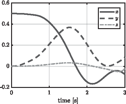
Here, as an illustrative example, we perform the dynamic simulation of a cantilever soft arm during a helical motion. This is possible by actuating the arm with a variable torque and a force as illustrated in Figure 4. The load conditions produce bending and torsion solicitations. The torque and force follow an $S -$ shaped profile for 3 s, with $f (0) = 0 N; f (3) = 2 N; τ (0) = 0 N \cdot m; τ (3) = 7 N \cdot m$ . The cross section properties are $E A = G A = 1 \times 1 0^{3} N$ , $E I = G J = 1 N \cdot m^{2}$ , $ρ A = 1 \times 1 0^{- 1} k g \cdot m^{- 1}$ , $ρ J = 2 k g \cdot m$ , $ρ I = 1 k g \cdot m$ . The length of the arm is $L = 1$ m. A snapshot of the simulation, taken at the temporal instant $t = 3$ s, is given in Figure 5. The capture shows the helical shape of the arm. The displacements of the free end of the arm along the three directions for the duration of the simulation are plotted in Figure 6. The motion of the arm is clearly three-dimensional.

FIG. 4.

Cantilever soft arm subjected to variable end loads.

FIG. 5.

Snapshot of the soft arm in helical motion, at t = 3 s.

FIG. 6.

Displacements of free end of the soft arm in helical motion.

In the following we present two different examples of arms in helical motion, an elastic rod made of spring steel and a hyperelastic body made of silicone. The main objective of these examples is to demonstrate the capability of the model to handle geometric nonlinearities with different settings of materials and cross sections of the arms. The first example simulates the behavior of a microscale and highly flexible system that can be used for minimally invasive robotic surgery applications. Indeed, the second example simulates the behavior of hyperelastic soft materials usually used in soft robotics applications as in robotic rehabilitation.

Elastic steel rod

The helical motion simulation is replicated here for an elastic rod made of spring steel. The torque and force follow a linear profile with $f (t) = 0.14 t$ N and $τ (t) = 0.49 t$ N·m. The motion is observed for 3 s. The cross section is circular, with diameter $d =$ 2 × 10⁻³ m, whereas the length is $L = 0.5$ m. The material properties are density $ρ = 7850 k g \cdot m^{- 3}$ , Young's modulus $E = 210$ GPa, Poisson's ratio $ν = 0.3$ , and shear modulus $G = E ∕ 2 (1 + ν)$ . The displacements of the free end of the arm along the three directions for the duration of the simulation are plotted in Figure 7.

FIG. 7.

Displacements of free end of the elastic steel rod in helical motion.

Elastic silicone body

The helical motion simulation is replicated here for a silicone body. The force and torque follow a linear profile with $f (t) = 0.1035 t$ N and $τ (t) = 0.01225 t$ N·m, respectively. The motion is observed again for 3 s. The cross section is circular, with diameter $d =$ 5 × 10⁻² m, whereas the length is again $L = 0.5$ m. The material properties are density $ρ = 1080 k g \cdot m^{- 3}$ , Young's modulus $E = 110$ kPa, Poisson's ratio $ν = 0.5$ , and shear modulus $G = E ∕ 2 (1 + ν)$ . The displacements of the free end of the arm along the three directions for the duration of the simulation are plotted in Figure 8.

FIG. 8.

Displacements of free end of the hyperelastic silicone body in helical motion.

Special Cases

In this section, starting from the geometrically exact model, we present two special cases, namely the planar bending of a soft arm in static conditions and the planar rotation of a soft arm in dynamic conditions. For these special cases, analytical solutions exist (the static solutions can be found in Ref.⁵⁶); here, we show how the deformation space model fits to these solutions.

Planar bending

Let us consider a cantilever soft arm actuated by a constant end torque $τ$ . Since the arm is clamped at the origin, we have that $δ h (0) = 0_{6 \times 1}$ , while the boundary conditions in the free end are $σ (L) = K (L) ε (L) = g_{e x t},$ (74)

where we consider the arm made of linear elastic material. We assume constant mass and stiffness cross section properties as well as constant initial curvature and torsion of the reference curve. Under these hypotheses, $f^{0}$ and $K$ are constant over the length of the arm.

Deformation field

The equilibrium equations in the static configuration expressed by Eq. (17) become $K ε^{'} - {\hat{f^{0}}}^{T} K ε = 0_{6 \times 1},$ (75)

where we used the fact that the stiffness matrix is constant over the arm. In this case, the solution for the deformation field can be expressed in closed form and it is given by $ε (α) = K^{- 1} F (α) K ε_{0},$ (76)

where $ε_{0}$ , the deformation at $α = 0$ , is a constant of integration and $F (α) = [\begin{array}{l} L^{T} (α) & 0_{3 \times 3} \\ {(T_{S O (3)} (α f_{ω}^{0}) α f_{u}^{0})}^{~} L^{T} (α) & L^{T} (α) \end{array}]$ (77)

with $L (α) = {exp}_{S O (3)} (α f_{ω}^{0})$ . Indeed, the tangent operator $T_{S O (3)} (\cdot)$ is given in Eq. (130). Inserting Eq. (76), computed at $α = L$ , into the boundary condition given by Eq. (74) yields $σ (L) = K K^{- 1} F (L) K ε_{0} = g_{e x t} (L)$ (78)

therefore, the constant of integration $ε_{0}$ is given by $ε_{0} = K^{- 1} {(F (L))}^{- 1} g_{e x t} (L) .$ (79)

by introducing Eq. (79) in Eq. (76), the solution for the deformation field reads $ε (α) = K^{- 1} F (α) {(F (L))}^{- 1} g_{e x t} (L) .$ (80)

In the special cases of pure bending/torsion solicitations, the external forces are given by $g_{e x t, u} (L) = 0_{3 \times 1}$ (81) $g_{e x t, ω} (L) = τ a$ (82)

where $τ \in ℛ$ and $a \in ℛ^{3}$ is an arbitrary vector. For an initially straight arm, we have $F (α) {(F (L))}^{- 1} = I_{6 \times 6}$ . Hence, the deformation field in Eq. (80) becomes $ε = K^{- 1} [\begin{matrix} 0_{3 \times 1} \\ τ a \end{matrix}] .$ (83)

Thus, it results that $ε$ is constant along the continuum arm. By separating the position and the orientation parts of the strains, the solution reads $[\begin{matrix} γ \\ κ \end{matrix}] = [\begin{matrix} 0_{3 \times 1} \\ K_{ω ω}^{- 1} (τ a) \end{matrix}] .$ (84)

$S E (3)$ field

The position and orientation fields are obtained by solving the kinematic equations in Eq. (3). Since the deformation field obtained in Eq. (83) involves constant strains, Eq. (3) can be integrated analytically and the solution for the $S E (3)$ field is exactly given by $H (α) = H_{0} e x p_{S E (3)} (α (f^{0} + ε)),$ (85)

which is equivalent to the forward kinematics mapping obtained in (26). Explicitly, Eq. (85) means $u (α) = u_{0} + R_{0} T_{S O (3)}^{T} (α (f_{ω}^{0} + κ)) α (f_{u}^{0} + γ)$ (86)

R (α) = R_{0} {exp}_{S 0 (3)} (α (f_{ω}^{0} + κ)) .

(87)

Since we are considering initially a straight arm, we have that $u_{0} = 0_{3 \times 1}$ , $R_{0} = I_{3 \times 3}$ and $f_{u}^{0} = {[1 0 0]}^{T}$ , $f_{ω}^{0} = 0_{3 \times 1}$ .

Let us consider a pure bending tip load as $g_{e x t, ω} (L) = τ [0 1 0]^{T}$ . According to Eq. (84), the deformations are given by $γ = {[\begin{matrix} 0 & 0 & 0 \end{matrix}]}^{T}$ (88)

κ = {[\begin{matrix} 0 & κ_{y} & 0 \end{matrix}]}^{T},

(89)

where $κ_{y} = τ ∕ (E I_{y})$ . Indeed, according to Eqs. (86)–(87), the position and rotation fields are given by $\begin{matrix} u (α) = [\begin{matrix} \frac{1}{κ_{y}} sin (α κ_{y}) \\ 0 \\ - \frac{1}{κ_{y}} (1 - cos (α κ_{y})) \end{matrix}] \end{matrix}$ (90)

R (α) = [\begin{matrix} cos (α κ_{y}) & 0 & sin (α κ_{y}) \\ 0 & 1 & 0 \\ - sin (α κ_{y}) & 0 & cos (α κ_{y}) \end{matrix}],

(91)

which is the exact solution expected from the special Cosserat rod theory.⁵⁷ A similar solution has been derived in the constant curvature framework for continuum robots.²⁶ Notice that in this example, the constant strains are not an assumption, but it comes out from the external load and boundary conditions. Since the exact analytical solution for the position and orientation field of the arm in a pure bending configuration is a curve of constant curvature, and since the kinematics in Eq. (27) contains this exact solution, the deformation space model is exact in pure bending configurations. The same happens in pure torsion configurations, where the exact solution for the $S E (3)$ field involves a curve of constant torsion. The configurations of the arm, with properties $E I_{2} = 1 N \cdot m^{2}$ and $L = 1$ m subject to five torques $τ = 1, 2, 3, 4, 5$ N·m, are given in Figure 9. Identical results are obtained for the analytical and the discrete models.

FIG. 9.

Static configuration of a cantilever soft arm in pure bending.

Planar rotation

Let us consider the soft arm shown in Figure 10 that is free to rotate at a constant velocity $ω_{0}$ in its own plane xz. The arm is initially straight, that is, $f_{u}^{0} = e_{1}$ and $f_{ω}^{0} = 0_{3 \times 1}$ . The coordinate along the arm, $α$ , ranges from $[0, L]$ , L being the length of the arm. The mass and stiffness matrices of the cross section are given, respectively, by $M = ρ d i a g (A, A, A, J, I_{2}, I_{3})$ and $K = d i a g (E A, G A_{2}, G A_{3}, G J, E I_{2}, E I_{3})$ . The arm is not subject to any external load, that is, $g_{e x t} = 0_{6 \times 1}$ . The boundary conditions are given by

FIG. 10.

Schematic model of a free rotating soft arm.

ε (L, t) = ε (0, t) = 0_{6 \times 1} .

(92)

Due to the centrifugal forces, it is expected that the arm is stretched. Accordingly, we have $γ = {[γ_{1} 00]}^{T}$ , $κ = 0_{3 \times 1}$ , $ν = {[\begin{matrix} 0 & 0 & v_{3} \end{matrix}]}^{T}$ , $ω = {[\begin{matrix} 0 & ω & 0 \end{matrix}]}^{T}$ .

Deformation and velocity fields

The deformation and velocity fields are obtained by solving the dynamics and compatibility equations. The dynamic equations in Eq. (25) become $ρ A v_{3} ω - E A_{γ^{'} 1} = 0$ (93)

x ρ A {\dot{v}}_{3} = 0

(94)

J \dot{ω} = 0,

(95)

while the compatibility equations in Eq. (6) become ${\dot{γ}}_{1} = 0$ (96)

v_{3}^{'} + ω (1 + γ_{1}) = 0

(97)

ω' = 0 .

(98)

Eq. (95) and Eq. (98) lead to $ω (α, t) = ω_{0} .$ (99)

Deriving Eq. (93) with respect to α and replacing the expression of $v'_{3}$ from Eq. (97) yield $E γ''_{1} + ρ ω_{0}^{2} γ_{1} = - ρ ω_{0}^{2} .$ (100)

The solution of Eq. (100), setting $c_{0} = \sqrt{ρ ∕ E}$ , is $γ_{1} (α) = a c o s (c_{0} ω_{0} (α + b)) - 1,$ (101)

where a and b are two constants of integration. By using the boundary conditions $γ_{1} (0) = γ_{1} (L) = 0$ , we obtain $a = \frac{1}{c o s (c_{0} ω_{0} L ∕ 2)}; b = - L ∕ 2 .$ (102)

Inserting the resulting expression of $γ_{1}$ into Eq. (93), we obtain the value of v₃ as $v_{3} = - \frac{a}{c_{0}} s i n (c_{0} ω_{0} (α + b)) .$ (103)

Finally, the expressions for v₃ and $γ_{1}$ are given by $v_{3} (α, t) = \frac{s i n (c_{0} ω_{0} (L ∕ 2 - α))}{c_{0} cos (c_{0} ω_{0} L ∕ 2)}$ (104)

γ_{1} (α, t) = \frac{cos (c_{0} ω_{0} (α - L ∕ 2))}{cos (c_{0} ω_{0} L ∕ 2)} - 1 .

(105)

Notice that $v_{3} (L ∕ 2) = 0$ : this means that the arm rotates about a fixed point, namely the material point at its mid-span.

SE(3) field

Integration of Eq. (5) leads to $R (t) = R_{0} e x p_{S O (3)} (ω t) = [\begin{matrix} c o s (ω_{0} t) & 0 & s i n (ω_{0} t) \\ 0 & 1 & 0 \\ - s i n (ω_{0} t) & 0 & c o s (ω_{0} t) \end{matrix}]$ (106)

for the orientation part and $u (α, t) = u_{0} + R_{0} [\begin{matrix} \frac{c o s (ω_{0} t) s i n (c_{0} ω_{0} (α - L ∕ 2))}{c_{0} ω_{0} c o s (c_{0} ω_{0} L ∕ 2)} \\ 0 \\ - \frac{s i n (ω_{0} t) s i n (c_{0} ω_{0} (α - L ∕ 2))}{c_{0} ω_{0} c o s (c_{0} ω_{0} L ∕ 2)} \end{matrix}]$ (107)

for the position part. Again, the integration of the kinematic equations is possible using the exponential operator.

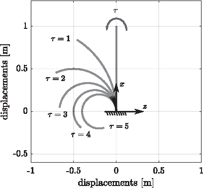
Let us consider the model in Figure 10 with $ρ = 2.7 \times 1 0^{- 3}$ kg·m⁻³, $E = 6.9 \times 1 0^{7}$ N · m⁻², $L = 1$ m subject to three angular velocities $ω_{0} = π, 2 π, 3 π$ rads⁻¹. The motion of the arm is observed for 1s. Figure 11 shows the displacements of node B during the simulation, for the exact analytical solution (solid lines) and the discrete solution (dotted lines), and we observe an almost exact matching of the two solutions. We define an average percentage error e given by

FIG. 11.

Displacements of node B of the free rotating soft arm. Color images are available online.

e (t) [%] = \frac{1}{2} \frac{x (t) - x_{e} (t)}{x_{e} (t)} \cdot 100 + \frac{1}{2} \frac{z (t) - z_{e} (t)}{z_{e} (t)} \cdot 100,

(108)

where $x_{e} (t)$ and $z_{e} (t)$ indicate the exact displacements given by the analytical solution. The errors along the trajectories, for the three simulations, are plotted in Figure 12. As we expected from the previous graph, the percentage errors, even if they increase by increasing the velocity, are all <0.1%.

FIG. 12.

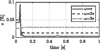
Errors of the free rotating soft arm.

Experimental Validation

Experimental setup

We replicate in simulation the Princeton experiment given in Ref.⁵⁸ The schematic model of the setup is shown in Figure 13. It comprises a cantilever arm subject to a tip load f, with variable lines of action according to the different values of the loading angle θ. Variation of the loading angle from 0 to 90 degrees yields out-of-plane motions with high nonlinear problems due to the fact that bending, torsion, and shear in two directions are coupled. The system is subject to gravity downward the z direction. 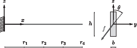The length of the arm is $L = 0.508$ m, whereas the dimensions of the rectangular cross section are thickness $b = 3.2024 m^{- 3}$ and height $h = 12.377 m^{- 3}$ . The arm is made of aluminum T 7075, with density $ρ = 2679 k g \cdot m^{- 3}$ , Young's modulus $E = 71.7$ GPa, Poisson's ratio $ν = 0.31$ , and shear modulus $G = 27.37$ GPa. The sectional mass matrix is given by

FIG. 13.

Schematic model of the Princeton experiment.

\begin{array}{l} \begin{matrix} M & = diag (ρ A, ρ A, ρ A, ρ J, ρ I_{y}, ρ I_{z}) = \\ = diag (0.1062 kg \cdot m^{- 1}, 0.1062 kg \cdot m^{- 1}, 0.1062 kg \cdot m^{- 1}, \\ \dots 3.034 \times 10^{- 6} kg \cdot m, 1.356 \times 10^{- 6} kg \cdot m, \end{matrix} \\ \dots 0.09078 \times 10^{- 6} kg \cdot m), \end{array}

(109)

where $A = b h$ is the area of the cross section, $I_{y} = \frac{b h^{3}}{12}$ and $I_{z} = \frac{h b^{3}}{12}$ are the area moment of inertia, and $J \approx h b^{3} (\frac{1}{3} - 0.21 \frac{b}{h} (1 - \frac{b^{4}}{12 h^{4}}))$ is used as an approximate solution of the torsion constant for rectangular cross sections.⁵⁹ Indeed, the sectional stiffness matrix is given by $\begin{matrix} K & = diag (E A, G A_{y}, G A_{z}, G J, E I_{y}, E I_{z}) = \\ = diag (2.842 \times 10^{6} N, 0.6401 \times 10^{6} N, 0.9039 \times 10^{6} N, \dots, \\ \dots 3.104 N \cdot m^{2}, 36.28 N \cdot m^{2}, 2.429 N \cdot m^{2}) \end{matrix}$ (110)

where $A_{y} = k_{y} A$ and $A_{z} = k_{z} A$ , $k_{y} = 0.590$ and $k_{z} = 0.833$ being the shear coefficients.⁶⁰ By setting $f_{0} = 4.448$ N, three or four load conditions are simulated for each loading angle as follows:

$f_{1} = f_{0}, f_{2} = 2 f_{0}, f_{3} = 3 f_{0}$ and $f_{4} = 4 f_{0}$ for $θ = 0, 15, 30$ degrees;

$f_{1} = f_{0}, f_{2} = 2 f_{0}, f_{3} = 3 f_{0}$ for $θ = 45$ degree;

$f_{1} = 1 ∕ 2 f_{0}, f_{2} = f_{0}, f_{3} = 3 ∕ 2 f_{0}$ and $f_{4} = 2 f_{0}$ for $θ = 60$ degree;

$f_{1} = 1 ∕ 2 f_{0}, f_{2} = f_{0}, f_{3} = 3 ∕ 2 f_{0}$ for $θ = 75, 90$ degrees

Experimental results consist of measurements of the two deflections of the cross section's dimensions of the arm (along y and z axes) at four radial stations $r_{i}, i = 1, \dots, 4$ along the longitudinal axis of the arm (x). Data were acquired at loading angles of $θ = 0, \pm 15, \pm 30, \pm 45, \pm 60, \pm 75 a n d \pm 90$ degrees with measurement accuracy in the order of hundredth of millimeter for the z direction and of tenth of millimeter for the y direction.⁵⁸ For a perfect system, symmetry implies that the absolute values of the deflections should be identical for loading angles $\pm θ$ . However, in these experimental settings, these measurements differ. Let us indicate with $y_{e i}^{+}$ and $z_{e i}^{+}$ the experimental measurements along y and z at $+ θ$ , with $y_{e i}^{-}$ and $z_{e i}^{-}$ the experimental measurements along y and z at $- θ$ and with $y_{e i}$ and $z_{e i}$ their average value. We define a percentage average variation index ${\bar{m}}_{i} [%]$ of the experimental measures normalized at each radial station r_i as ${\bar{m}}_{i} [%] = (\frac{| y_{e i}^{+} - y_{e i} |}{r_{i}} + \frac{| y_{e i}^{-} - y_{e i} |}{r_{i}} + \frac{| z_{e i}^{+} - z_{e i} |}{r_{i}} + \frac{| z_{e i}^{-} - z_{e i} |}{r_{i}}) \cdot 100$ (111)

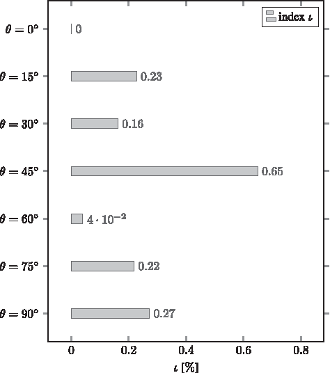
To achieve a synthetic index on the variations of the experimental measures, we calculate Eq. (111) for each radial station and loading condition, with fixed loading angle. Then, we compute their standard deviations: the result is the index $ι$ that summarizes the variations of the experimental measures for all the loading angles (Fig. 14). By averaging all these seven values, we obtain an average index $ι$ for all the experimental data sets, equal to $0.224 %$ .

FIG. 14.

Variations of the experimental measurements.

Definition of the errors

The same external loading conditions of the experiments, including the applied forces and the gravity effects, were replicated in simulation. Then, the deflections of the cross section axes (along y and z) at $r_{1}, r_{2}, r_{3}$ , and r₄ were compared. To evaluate the accuracy of the model, we need to define an error measure

We define a percentage error $e_{i} [%]$ as the normalized distance between the simulated and experimental deflections at each radial station as $e_{i} [%] = (\frac{|y (r_{i}) - y_{e i}|}{r_{i}} + \frac{|z (r_{i}) - z_{e i}|}{r_{i}}) \cdot 100,$ (112)

where $y_{e i}$ and $z_{e i}$ indicate the averaged experimental deflections, whereas $y (r_{i})$ and $z (r_{i})$ indicate the simulated deflections. Furthermore, we indicate with $e_{μ}$ and $e_{δ}$ , respectively, the mean and the standard deviation of the four errors along the arm's length, for each loading condition.

Results

A total of 25 simulations were conducted and the 100 comparisons with the experimental data give satisfactory results.

$θ = 0$ degree

In-plane motion in the plane xz (Fig. 15a). The errors defined in Eq. (112) are shown in Figure 16a.

FIG. 15.

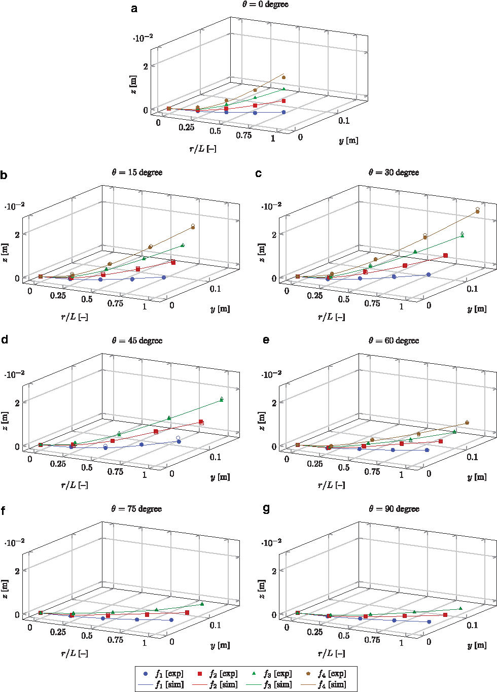
Deflections of the cross section dimensions for the Princeton experiment. Solid lines, simulated data; scattered lines, experimental data (filled, +θ; nonfilled, −θ). Color images are available online.

FIG. 16.

Normalized Euclidean errors between the averaged experimental data and simulated data for the different load conditions. Color images are available online.

$θ = 15$ degree

Out-of-plane three-dimensional motion (Fig. 15b). The errors defined in Eq. (112) are shown in Figure 16b.

$θ = 30$ degree

Out-of-plane three-dimensional motion (Fig. 15c). The errors defined in Eq. (112) are shown in Figure 16c.

$θ = 45$ degree

Out-of-plane three-dimensional motion (Fig. 15d). Notice that the experiment with $f_{4} = 4 f_{0}$ was not performed with this loading angle so as to not physically damage the experimental apparatus. The errors defined in Eq. (112) are shown in Figure 16d.

$θ = 60$ degree

Out-of-plane three-dimensional motion (Fig. 15e). Notice that the four loading conditions are with half of the intensity with this loading angle, according to Experimental Setup section, in order to avoid physical damages on the experimental apparatus. The errors defined in Eq. (112) are shown in Figure 16e.

$θ = 75$ degree

Out-of-plane three-dimensional motion (Fig. 15f). In this study, the experiment with $f_{4} = 2 f_{0}$ was not performed for the same reason already described. The errors defined in Eq. (112) are reported in Figure 16f.

$θ = 90$ degree

In-plane motion in the plane xy (Fig. 15g). In this study, again the experiment with $f_{4} = 2 f_{0}$ was not performed. The errors defined in Eq. (112) are shown in Figure 16g for the last loading condition.

Discussion

Figure 15 shows the shapes of the arm under the applied loads, for all loading angles. The solid lines indicate the simulated responses, whereas the scattered lines indicate the experimental responses, for loading angles $+ θ$ (filled scatter) and loading angles $- θ$ (nonfilled scatter). As we can observe from this figure, the shape of the simulated arm closely matches the experimental responses, with errors that are all < $1 %$ , as we can see in Figure 16.

As we can expect, for each loading angle, the general trend is a slight increase of the errors when the intensity of the load increases.

However, if we compare the two extreme cases, that is, $θ = 0$ degree and $θ = 90$ degree, which correspond to two in-plane motions, respectively, in the planes xz and yz, the latter presents higher errors, even if the intensity of the load is lower. The Princeton arm has a more stiff behavior along the z direction, since the bending stiffness about the y axis is higher if compared with the bending stiffness about the z axis [Eq. (111)]. The higher measurement accuracy of the data set for the z direction might be the cause of this discrepancy. As a matter of fact, the model better reflects the deflections along the z direction. However, the errors in predicting the deflections along the more compliant direction, namely the y axis, even if bigger, are < $0.4 %$ (for this comparison, see Fig. 16).

From the available measurements, we can observe higher errors when the load increases, and when the loading conditions produce the majority of motion in the more compliant directions. But, since in the latter cases the experiments were performed with forces of lower intensity so as to not compromise the experimental apparatus, all the errors in this set of experiments span in the small range 0–0.6%.

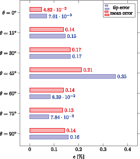
It is interesting to notice than the tip errors (corresponding to $r ∕ L = 1$ ) are comparable with the errors along the arm's length. This means that the model can accurately predict the deflections of the worst case cross section. In this respect, we show in Figure 17 a synthesis of Figure 16, focusing the attention on the mean errors and tip errors, which are the average values of $e_{μ}$ and e₄, respectively, for all the loading conditions. Furthermore, in Figure 18 the standard deviation values of these errors are shown. From these plots, we can have a synthetic view of the average errors of the model. By averaging all the seven values of this plot, we obtain an average mean error of $0.140 % \pm 0.072 %$ and an average tip error of $0.151 % \pm 0.102 %$ .

FIG. 17.

Experimental validation results (errors). Color images are available online.

FIG. 18.

Experimental validation results (standard deviations of the errors). Color images are available online.

Notice that the standard deviations of these errors (reported with respect to the averaged experimental deflections) are the same order of magnitude of the $ι$ indices: hence, we can state we have numerical results within the range of variability of the experimental measurements.

The tip errors were calculated to provide a more common accuracy index for the robotic community, even if in the case of soft robots we are interested in all the points along the configuration of the manipulator.

Application Scenarios

The main advantages that historically have motivated the development of soft and continuum robots are their ability to⁶¹:

access remotely in complex environments: this ability is appealing in maintenance, inspection, and repair operations, and in minimally invasive surgery;

adapt their shape to perform whole-limb manipulation: soft robots might help in applications that require a safe physical human–robot interaction, as in industry or in rehabilitation.

Therefore, we select two scenarios in which the use of such robotic systems is of current interest: surgical and rehabilitation. For these applications, we just set up the model and perform simulations that reflect typical motions of these systems.

Surgical

The Magellan™ Robotic Catheter 10Fr has been selected for this analysis (www.hansenmedical.com). This is a robotic catheter used for intravascular shaping operations, and it is composed of a guide and a robotically steerable inner leader. Both the guide and the leader have the possibility to bend. In the case of minimal extension of the leader, the catheter is composed of two consecutive elements (1–2, the guide and 2–3, the leader) as we can see from the schematic representation of Figure 19. 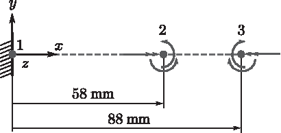The guide and the leader are made of spring steel, with density $ρ = 7850 k g m^{- 3}$ , Young's modulus $E = 210$ GPa, Poisson's ratio $ν = 0.3$ , and shear modulus $G = E ∕ 2 (1 + ν)$ . The cross sections are circular crowns with the following dimensions for the guide: external diameter $d_{e, g} = 3.48 \times 1 0^{- 3} m$ and internal diameter $d_{i, g} = 2.54 \times 1 0^{- 3} m$ ; for the leader: $d_{e, l} = 2.13 \times 1 0^{- 3} m$ and internal diameter $d_{i, g} = 1.00 \times 1 0^{- 3} m$ . As illustrative example, we consider the following actuation loads applied at the end of the guide (2) and at the end of the leader (3):

FIG. 19.

Magellan Robotic Catheter 10Fr in the configuration of minimum extension of the leader (only flexible parts shown). Schematic model.

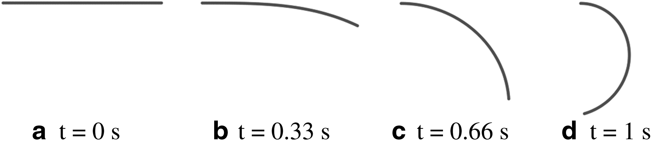
\begin{matrix} ∙ τ_{2, x} = 0.4 t N \cdot m; τ_{2, y} = 4 t N \cdot m; τ_{2, z} = 40 t N \cdot m, \\ 0 \leq t \leq 1 s . 3 \end{matrix}

\begin{matrix} ∙ τ_{3, x} = - 0.15 t N \cdot m; τ_{3, y} = - 1.5 t N \cdot m; \\ τ_{3, z} = - 15 t N \cdot m, 0 \leq t \leq 1 s . \end{matrix}

The actuation load induces an out-of-plane motion of the robotic catheter, which is typical in robotic steerable shaping operations, resulting in both bending and torsion. Some snapshots of the model in SimSOFT during the simulation are shown in Figure 20a–d.

FIG. 20.

Magellan Robotic Catheter 10Fr in the configuration of minimum extension of the leader (only flexible parts shown). Snapshots of the simulation in SimSOFT.

Rehabilitation

A soft body subjected to bending and made of elastomeric material has been selected for this analysis. This can approximate the soft bending actuators that are used in the development of soft orthotics and/or prosthetics for rehabilitation purposes. The schematic representation of the system is shown in Figure 21. The length of the body is $L = 0.15$ m, the cross section is a solid semicircle, with $r = 1 \times 1 0^{- 2} m$ . The material properties are density $ρ = 1080 k g \cdot m^{- 3}$ , Young's modulus $E = 110$ kPa, Poisson's ratio $ν = 0.5$ , and shear modulus $G = E ∕ 2 (1 + ν)$ . As illustrative example, we apply a torque $τ (t) = 0.002 t$ N m about y direction and we observe the motion for 1 s. The torque induces an in-plane motion, which is typical in whole-limb manipulation. Some snapshots of the model in SimSOFT are shown in Figure 22a–d.

FIG. 21.

Schematic model of the soft silicone body with applied torque.

FIG. 22.

Snapshots of the soft silicone body with applied torque in SimSOFT.

Conclusion

In this article, geometrically exact models for the kinematics, statics, and dynamics of soft robots have been derived. They account for the large deformations due to bending, torsion, shear, and extension. The models build on top of the theory of continuum Cosserat rods, whose partial differential dynamic equations are formulated on a Lie group. The spatial discretization was achieved, in a finite element manner, using helical shape functions that mathematically are represented by the exponential mapping. From this, the forward and inverse kinematics of the arm were derived, accounting for robot with straight or curve initial configuration. The subsequent derivation of the soft geometric Jacobian allowed the description of the differential kinematics of the robot. Then, the statics was derived using the principle of virtual work, whereas the dynamics was derived from the Hamilton's principle. Finally, the equations of motion were numerically solved using a geometric time integration scheme, the Lie group version of the generalized $α$ scheme.

We validated the discrete model with two analytic examples, namely the pure bending of a cantilever soft arm and the pure rotation of a soft arm in the plane, with varying external conditions. We performed an experimental validation with respect to the Princeton arm, which represents an excellent benchmark for testing models where bending, torsion, and shear are coupled. A total of 25 simulations corresponding to 100 averaged experimental positions were replicated. The results show an average tip distance between the real and simulated robot of 1.32 mm, whereas the errors in all the performed simulations are far < $1 %$ . These experiments represent only the starting point for further investigations on other real systems. Furthermore, some examples and applications are presented to demonstrate the capability of the model in simulating soft robots with different materials and cross section properties. Even if this article deals with geometric nonlinearities, further work has been planned to model material nonlinearities as well.

The models derived in this article, for the first time in the soft robotics community, combine a geometric spatial integration with a geometric time integration. Thus, they can effectively be considered full geometric models. Furthermore, the finite element method allows a straightforward implementation of concatenated elements.

The average computational time required for solving 1 s of simulation, with time step size of 0.01 s, is 2 s. This significantly improves previous results in the field, and it is promising toward a real-time model-based reconstruction of the robot shape in dynamic conditions. Furthermore, the full geometric models discussed in this article might pave the way for model-based controllers, enabling the shape control of this class of robotic manipulators.

Finally, the computer implementation of the models described in this work has led to SimSOFT, a software library for soft robot modeling, which is in continuous development by the authors.

Footnotes

Acknowledgments

This work was partially supported by the FlexARM project, which has received funding from the European Commission's Euratom Research and Training Programme 2014–2018 under the EUROfusion Engineering Grant EEG-2015/21 and partially by the RoDyMan project, which has received funding from the European Research Council under Advanced Grant 320992.

Author Disclosure Statement

No competing financial interests exist.

Appendix A1: Nomenclature

( $\dot{\cdot}$ ) derivative with respect to time

(.)′ derivative with respect to space

$\tilde{(.)} ℝ^{6} \to s e (3)$

(., .) $s e (3) \times s e (3) \to s e (3)$

$\hat{(\cdot)} ℛ^{6} \to ℛ^{6 \times 6}$

t $\in ℛ$ , time

α $\in ℛ$ , reference curve parameterization

u $\in ℛ^{3}$ , position vector

R $\in S O (3)$ , rotation matrix

H $\in S E (3)$ , configuration matrix

η $\in ℛ^{6}$ , velocity vector

f $\in ℛ^{6}$ , deformation vector

σ $\in ℛ^{6}$ , stress vector

Appendix A2: Lie Group Framework

This Appendix reports some basic operations on a Lie group.

References

Trivedi

, Rahn

, Kier

, et al. Soft robotics: biological inspiration, state of the art, and future research. Appl Bionics Biomech, 2008; 5:99–117.

Majidi

. Soft robotics: a perspective current trends and prospects for the future. Soft Robot, 2014; 1:5–11.

Burgner-Kahrs

, Rucker

, Choset

. Continuum robots for medical applications: a survey. IEEE Trans Robot, 2015; 31:1261–1280.

Park

Y-L

, Chen

, Pérez-Arancibia

, et al. Design and control of a bio-inspired soft wearable robotic device for ankle–foot rehabilitation. Bioinspir Biomim, 2014; 9:016007.

Polygerinos

, Wang

, Galloway

, et al. Soft robotic glove for combined assistance and at-home rehabilitation. Rob Auton Syst, 2015; 73:135–143.

Buckingham

, Graham

. Reaching the unreachable-snake arm robots. In: Proceedings of the 43rd International Symposium on Robotics. Taipei, Taiwan:. 2012.

Grazioso

, Di Gironimo

, Iglesias

, et al. Screw-based dynamics of a serial/parallel flexible manipulator for demo blanket remote handling. Fusion Eng Des, 2018 (in press).

Mehling

, Diftler

, Chu

, et al. A minimally invasive tendril robot for in-space inspection. In: The First IEEE/RAS-EMBS International Conference on Biomedical Robotics and Biomechatronics. Pisa, Italy: IEEE, 2006, pp. 690–695.

Polygerinos

, Correll

, Morin

, et al. Soft robotics: review of fluid-driven intrinsically soft devices; manufacturing, sensing, control, and applications in human-robot interaction. Adv Eng Mater, 2017; 19:1700016.

10.

Rus

, Tolley

. Design, fabrication and control of soft robots. Nature, 2015; 521:467.

11.

Lipson

. Challenges and opportunities for design, simulation, and fabrication of soft robots. Soft Robot, 2014; 1:21–27.

12.

Hiller

, Lipson

. Automatic design and manufacture of soft robots. IEEE Trans Robot, 2012; 28:457–466.

13.

Tolley

, Shepherd

, Mosadegh

, et al. A resilient, untethered soft robot. Soft Robot, 2014; 1:213–223.

14.

Marchese

, Komorowski

, Onal

, et al. Design and control of a soft and continuously deformable 2 d robotic manipulation system. In: 2014 IEEE International Conference on Robotics and Automation. Hong Kong, China: IEEE, 2014, pp. 2189–2196.

15.

Marchese

, Tedrake

, Rus

. Dynamics and trajectory optimization for a soft spatial fluidic elastomer manipulator. Int J Rob Res, 2016; 35:1000–1019.

16.

Della Santina

, Bianchi

, Grioli

, et al. Controlling soft robots: balancing feedback and feedforward elements. IEEE Robot Autom Mag, 2017; 24:75–83.

17.

Thuruthel

, Ansari

, Falotico

, Laschi

. Control strategies for soft robotic manipulators: a survey. Soft Robot, 2018; 5:149–163.

18.

Della Santina

, Katzschmann

, Bicchi

, et al. Dynamic control of soft robots interacting with the environment. In: The first IEEE-RAS International Conference on Soft Robotics. Livorno, Italy: IEEE, 2018, pp. 46–53.

19.

Della Santina

, Lakatos

, Bicchi

, et al. Using nonlinear normal modes for execution of efficient cyclic motions in soft robots. arXiv preprint arXiv:1806.08389 2018.

20.

Amend

, Brown

, Rodenberg

, et al. A positive pressure universal gripper based on the jamming of granular material. IEEE Trans Robot, 2012; 28:341–350.

21.

Della Santina

, Grioli

, Catalano

, et al. Dexterity augmentation on a synergistic hand: the pisa/iit softhand+. In: 2015 IEEE-RAS 15th International Conference on Humanoid Robots. Seoul, South Korea: IEEE, 2015, pp. 497–503.

22.

Deimel

, Brock

. A novel type of compliant and underactuated robotic hand for dexterous grasping. Int J Rob Res, 2016; 35:161–185.

23.

Saunders

, Trimmer

, Rife

. Modeling locomotion of a soft-bodied arthropod using inverse dynamics. Bioinspir Biomim, 2010; 6:016001.

24.

Shepherd

, Ilievski

, Choi

, et al. Multigait soft robot. Proc Natl Acad Sci U S A, 2011; 108:20400–20403.

25.

Marchese

, Onal

, Rus

. Autonomous soft robotic fish capable of escape maneuvers using fluidic elastomer actuators. Soft Robot, 2014; 1:75–87.

26.

Webster RJ

III

, Jones

. Design and kinematic modeling of constant curvature continuum robots: a review. Int J Rob Res, 2010; 29:1661–1683.

27.

Jones

, Walker

. Kinematics for multisection continuum robots. IEEE Trans Robot, 2006; 22:43–55.

28.

Neppalli

, Csencsits

, Jones

, et al. Closed-form inverse kinematics for continuum manipulators. Adv Robot, 2009; 23:2077–2091.

29.

Simaan

, Xu

, Wei

, et al. Design and integration of a telerobotic system for minimally invasive surgery of the throat. Int J Rob Res, 2009; 28:1134–1153.

30.

Grazioso

, Sonneville

, Di Gironimo

, et al. A nonlinear finite element formalism for modelling flexible and soft manipulators. In: IEEE International Conference on Simulation, Modeling, and Programming for Autonomous Robots. San Francisco, CA: IEEE, 2016, pp. 185–190.

31.

, Simaan

. Analytic formulation for kinematics, statics, and shape restoration of multibackbone continuum robots via elliptic integrals. J Mech Robot, 2010; 2:011006.

32.

Selig

, Ding

. A screw theory of timoshenko beams. J Appl Mech, 2009; 76:031003.

33.

Simo

. A finite strain beam formulation. The three-dimensional dynamic problem. Part I. Comput Methods Appl Mech Eng, 1985; 49:55–70.

34.

Simo

, Vu-Quoc

. A three-dimensional finite-strain rod model. Part II: computational aspects. Comput Methods Appl Mech Eng, 1986; 58:79–116.

35.

Borri

, Bottasso

. An intrinsic beam model based on a helicoidal approximation part i: formulation. Int J Numer Methods Eng, 1994; 37:2267–2289.

36.

Borri

, Bottasso

. An intrinsic beam model based on a helicoidal approximation part ii: linearization and finite element implementation. Int J Numer Methods Eng, 1994; 37:2291–2309.

37.

Cardona

, Geradin

. A beam finite element non-linear theory with finite rotations. Int J Numer Methods Eng, 1988; 26:2403–2438.

38.

Jelenić

, Crisfield

. Geometrically exact 3 d beam theory: implementation of a strain-invariant finite element for statics and dynamics. Comput Methods Appl Mech Eng, 1999; 171:141–171.

39.

Sonneville

, Cardona

, Brüls

. Geometrically exact beam finite element formulated on the special Euclidean group SE(3). Comput Methods Appl Mech Eng, 2014; 268:451–474.

40.

Chirikjian

. Hyper-redundant manipulator dynamics: a continuum approximation. Adv Robot, 1994; 9:217–243.

41.

Boyer

, Porez

, Khalil

. Macro-continuous computed torque algorithm for a three-dimensional eel-like robot. IEEE Trans Robot, 2006; 22:763–775.

42.

Trivedi

, Lotfi

, Rahn

. Geometrically exact models for soft robotic manipulators. IEEE Trans Robot, 2008; 24:773–780.

43.

Rucker

, Jones

, Webster RJ

III

. A geometrically exact model for externally loaded concentric-tube continuum robots. IEEE Trans Robot, 2010; 26:769–780.

44.

Rucker

, Webster RJ

III

. Statics and dynamics of continuum robots with general tendon routing and external loading. IEEE Trans Robot, 2011; 27:1033–1044.

45.

Shampine

. Solving hyperbolic pdes in matlab. Appl Numer Anal Comput Math, 2005; 2:346–358.

46.

Laschi

, Cianchetti

, Mazzolai

, et al. Soft robot arm inspired by the octopus. Adv Robot, 2012; 26:709–727.

47.

Renda

, Giorelli

, Calisti

, et al. Dynamic model of a multibending soft robot arm driven by cables. IEEE Trans Robot, 2014; 30:1109–1122.

48.

Renda

, Boyer

, Dias

, Seneviratne

. Discrete Cosserat approach for multi-section soft robots dynamics. IEEE Trans Robot, 2018:1–16.

49.

Christensen

. Theory of Viscoelasticity: An Introduction. New York: Elsevier, 2012.

50.

Grazioso

, Di Gironimo

, Siciliano

. From differential geometry of curves to helical kinematics of continuum robots using exponential mapping. In: Lenarcic

, Parenti-Castelli

, eds. Advances in Robot Kinematics 2018. New York: Springer International Publishing, 2019, pp. 319–326.

51.

Park

, Chung

. Geometric integration on Euclidean group with application to articulated multibody systems. IEEE Trans Robot, 2005; 21:850–863.

52.

Brüls

, Cardona

, Arnold

. Lie group generalized-α time integration of constrained flexible multibody systems. Mech Mach Theory, 2012; 48:121–137.

53.

Terze

, Müller

, Zlatar

. Lie-group integration method for constrained multibody systems in state space. Multibody Syst Dyn, 2015; 34:275–305.

54.

Brüls

, Cardona

. On the use of lie group time integrators in multibody dynamics. J Comput Nonlinear Dyn, 2010; 5:031002.

55.

Demoures

, Gay-Balmaz

, Leyendecker

, et al. Discrete variational lie group formulation of geometrically exact beam dynamics. Numer Math, 2015; 130:73–123.

56.

Grazioso

, Di Gironimo

, Siciliano

. Analytic solutions for the static equilibrium configurations of externally loaded cantilever soft robotic arms. In: The first IEEE-RAS International Conference on Soft Robotics. Livorno, Italy: IEEE, 2018, pp. 140–145.

57.

Antman

SS.

Nonlinear Problems of Elasticity, volume 107. Springer Science & Business Media, 2005.

58.

Dowell

, Traybar

. An experimental study of the nonlinear stiffness of a rotor blade undergoing flap, lag and twist deformations. Princeton, NJ: Nasa Technical Report, Princeton University, 1995.

59.

Young

, Budnyas

. Roarks Formulas for Stress and Strain. New York: McGraw-Hill, 2017.

60.

Cowper

. The shear coefficient in timoshenkos beam theory. J Appl Mech, 1966; 33:335–340.

61.

Walker

, Choset

, Chirikjian

. Snake-like and continuum robots. In: Siciliano

, Oussama

, eds. Springer Handbook of Robotics. Cham, Switzerland: Springer, 2016, pp. 481–498.

A Geometrically Exact Model for Soft Continuum Robots: The Finite Element Deformation Space Formulation

Abstract

Introduction

Problem statement

Review of relevant literature

Contributions

Outline

Continuum Formulation

Position field

Deformation field

Velocity field

Compatibility equations

Strain energy

Static equilibrium equations

Kinetic energy

Dynamic equilibrium equations

The Finite Element Deformation Space Formulation

The finite element approach

Forward kinematics

Inverse kinematics

Differential kinematics

Statics

Dynamics

Time integration

SimSOFT

Geometrical Interpretation

Helical motion

Elastic steel rod

Elastic silicone body

Special Cases

Planar bending

Deformation field

S E 3 field

Planar rotation

Deformation and velocity fields

SE(3) field

Experimental Validation

Experimental setup

Definition of the errors

Results

θ = 0 degree

θ = 1 5 degree

θ = 3 0 degree

θ = 4 5 degree

θ = 6 0 degree

θ = 7 5 degree

θ = 9 0 degree

Discussion

Application Scenarios

Surgical

Rehabilitation

Conclusion

Footnotes

Acknowledgments

Author Disclosure Statement

Appendix A1: Nomenclature

Appendix A2: Lie Group Framework

References

$S E (3)$ field

$θ = 0$ degree

$θ = 15$ degree

$θ = 30$ degree

$θ = 45$ degree

$θ = 60$ degree

$θ = 75$ degree

$θ = 90$ degree