Modeling Dynamic PET-SPECT Studies in the Wavelet Domain

Abstract

This work develops a theoretical framework and corresponding algorithms for the modeling of dynamic PET-SPECT studies both in time and space.

The problem of estimating the spatial dimension is solved by applying the wavelet transform to each scan of the dynamic sequence and then performing the kinetic modeling and statistical analysis in the wavelet domain. On reconstruction through the inverse wavelet transform, one obtains parametric images that are consistent estimates of the spatial patterns of the kinetic parameter of interest.

The theoretical setup allows the use of linear techniques currently used in PET-SPECT for kinetic analysis. The method is applied to artificial and real data sets. The application to dynamic PET-SPECT studies was performed both for validation purposes, when the spatial patterns are known, and for illustration of the advantages offered by the technique in case of tracers with an unknown pattern of distribution.

Keywords

Estimation Kinetics Positron emission tomography Single photon emission computed tomography Wavelets

Dynamic studies are common in emission tomography (ET). They consist of the acquisition of a temporal sequence of scans that allows the measurement of the kinetic of a tracer; the ensuing application of an appropriate mathematical model to the time course of the measured radioactivity allows the estimation of a physiologic parameter of interest (Phelps et al., 1986).

It is common to apply the estimation process to the activity curve of each image element (pixel) so that an image of the distribution of the physiologic parameter (“parametric image”) is produced. However, the modeling process may not be considered complete if only the time-varying structure of images is considered. A more comprehensive description should represent the dynamic set of images as the measurement of a time-varying spatial pattern of radioactivity. By adding the spatial dimension to the kinetic model, one may obtain an estimate of the spatial pattern of the physiologic parameter of interest.

Spatial modeling may be relevant in the context of positron emission tomography (PET) and single photon emission computed tomography (SPECT). First, the introduction of a proper model for the spatial signal may enhance the quality of image denoising (Turkheimer et al., 1999). Second, if the estimation of the spatial model is carried out in a rigorous statistical framework, then one may be able to discriminate signal from noise within a desired risk of false positives (Turkheimer et al., 1999). The latter property is desirable when the pattern of distribution is not known a priori and signal-to-noise ratio is low.

A previous paper (Turkheimer et al., 1999) considered the problem of the estimation of spatial patterns of radioactivity acquired by ET. The problem was solved by use of the wavelet transform (WT), and theory and algorithms were provided that suited the application to PET and SPECT images. This work extends these results to dynamic studies by providing a framework where both wavelet and kinetic analysis can be performed.

This article defines the problem of modeling a time-varying spatial pattern of radioactivity and describes the new procedure for its estimation. The basics of WT in its discrete formulation, the dyadic wavelet transform (DWT), are surveyed. The limitations of the DWT in the context of PET-SPECT images are considered, and we discuss how they may be overcome by use of the translation-invariant dyadic wavelet transform (DWT-TI). The application of kinetic modeling in the wavelet domain is detailed, and we recall the problem of thresholding of wavelet coefficients and suggest two schemes that can be used in the kinetic modeling of ET dynamic scans.

Although the procedure is new, its basic ingredients were described previously (Turkheimer et al., 1999) and will not be dealt with in depth. The reader is also referred to Turkheimer et al. (1999) for an introduction to wavelets, related background material, definition of terms specific to the methodology, and notation. More recent references on wavelets are Härdle et al. (1998) and Vidakovic (1999) for the general topic and Nowak and Baraniuk (1999) for emission tomographs.

This article further describes the application of the procedure to several data sets. The aim of this section is twofold. First, the results of the technique are used for validation purposes when used for modeling patterns of activity that are well known in advance. This is the case of an artificial data set and dynamic PET studies with [¹⁸F]fluorodeoxyglucose (FDG) and [¹¹C]raclopride. On the other hand, the case of a dynamic [¹¹C](R)-PK11195 study illustrates the usefulness of the approach in the statistical detection of signal of unknown distribution.

The paper also contains an example of the analysis of a dynamic SPECT scan where the quantitative kinetic modeling is substituted by a nonquantitative principal component analysis (PCA). The emphasis here is on the versatility of the procedure, which enables the incorporation of any approach for the mathematical analysis of the time dimension.

MODELING A TIME-VARYING RADIOACTIVE PATTERN

Define ℕ to be the set of nonnegative integer numbers, ℝ to be the set of real numbers, and L²(ℝ) to be the space of squared integrable real functions (i.e., functions with finite energy). Let P(s) be the pattern of a physiologic parameter of interest where s ∈ ℕⁿ spans the sites where the process is measured by the scanner (i.e., s: s = (s_x,s_y) ∈ ℕ in the two-dimensional case of an image where s_x and s_y are the pixels' numbers) and P(s) ∈ L²(ℝ).

We are interested in the estimation of P(s) from a time-changing pattern of radioactivity V(s,t_i), where i ∈ ℕ and t_i runs through the M midframe times t = t₁, t₂, … t_M, and V(s,t₁), …, V(s,t_M) ∈ L²(ℝ). For example, P(s) may be the pattern of glucose metabolism and V(s,t_i) is the radioactive pattern of distribution of FDG in the field of view during the time window of the experiment.

V(s,t_i) is related to P(s) by a functional κ(•) that contains the description of the kinetic of the radioactive compound in terms of the biologic variable of interest. We can then write P(s) = κ(V(s,t_i)). κ(•) in ET is usually derived from compartmental models where the tracer is modeled with first-order kinetics.

Finally, consider that PET and SPECT measurements will be corrupted by noise and that only the noisy observations Y(s,t_i) = V(s,t_i) + e(s,t_i) will be available, where e(s,t₁), …, e(s,t_M) are the noise processes of each dynamic scan. In our analysis, images Y(s,t_i) are acquired from emission tomographs and reconstructed from sinograms or planar projections at their highest resolution using back-projection with a ramp filter. Therefore, we can assume e(s,t₁), …, e(s,t_M) to be independent, normally distributed with mean 0, unknown variance σ², and a local spatial correlation structure introduced by the reconstruction process (Turkheimer et al., 1999).

In the previous work (Turkheimer et al., 1999), the assumption was made for the noise process to be stationary-that is, the variance was supposed homogeneous across each emission image. Here this assumption is relaxed and variance is allowed to vary across time and space as σ² = σ²(s,t_i), with some constraints that will be detailed below.

Given the above, the problem of interest is the computation of an estimate P̂(s) from the dynamic data set Y(s,t₁), Y(s,t₂), …, Y(s,t_M) with small risk R (P̂, P) = E(∑_s|P̂(s) – P(s)|²), where E(•) is the expected value and ∑_s|P̂(s) – P (s)|² is the L₂-norm of least-square estimation.

ESTIMATING A PARAMETRIC PATTERN

The procedure is illustrated in Fig. 1 for a single slice of the image volume (two-dimensional case). In the diagram, Y(s,t_i) is the dynamic ET image sequence, and we desire to produce a parametric map P̂(s) that contains the estimated pattern of the parameter of interest. The scheme contains four steps. First, the DWT is applied to each image Y(s,t₁), Y(s,t₂), …, Y(s,t_M) and produces the correspondent wavelet transforms W(w,t₁), W(w,t₂), …, W(w,t_M). The DWT is a linear operator that expands the original image in terms of a scalable and shiftable elementary function, the wavelet. This means that the measured radioactivity is projected into a space where each coordinate represents a portion of the radioactive pattern at a certain scale in a certain location. This consideration drives naturally to the second step, where the usual kinetic modeling is applied to the time-curve of each wavelet coefficient. This means that for each coordinate w = [w_x, w_y], the coefficient P̂_wt(w) = κ(W(w,t_i)) is computed. The final outcome is a parametric wavelet transform P̂_wt(w). Note that for equivalence between wavelet and image space, all applied operators must be linear; therefore, κ(•) must be linear in the data too.

FIG. 1.

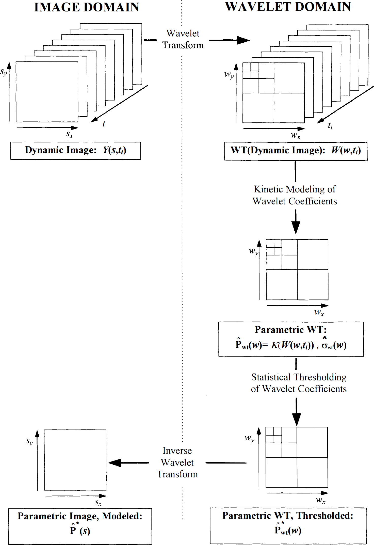
The four steps for estimating the pattern of distribution of the physiologic parameter of interest, here denoted as P(s), from the dynamic set of images Y(s,t₁). The wavelet transform is first applied to each time frame and the collection of transforms is denoted as W(w,t_i). The usual kinetic modeling is then implemented in the wavelet domain. The modeling process is represented by application of the functional κ(•) to the time course of each wavelet coefficient. This step results in the parametric wavelet transform P̂_wt(w_x,w_y) = κ(W(w_x,w_y,t_i)) and its corresponding standard error σ̂_wt((w_x,w_y). Wavelet coefficients are then thresholded and the remaining ones, P̂_wt(w_x,w_y), are passed through the inverse wavelet transform to produce the desired estimate P̂(s).

Two main features of the DWT enhance the application of modeling when applied in wavelet space. First, the DWT is a linear operator, and if e(s,t_i) is normally distributed in the image space, e(s,t_i) will be normally distributed in wavelet space (Donoho and Johnstone, 1994). Second, the DWT is a decorrelation operator, and the correlated noise processes in image space e(s,t₁), e(s,t₂), …, e(s,t_M) become the white noise processes e(w,t₁), e(w,t₂),…, e(w,t_M) in wavelet space (Johnstone and Silverman, 1997).

The possibility of having a model for the time-dependency of the coefficients of P(w) is an advantage also for the statistical treatment of wavelets. In fact, because the application of κ(•) usually results in a classic least-squares estimation procedure, one may be able to compute the uncertainty of each wavelet parametric coefficient P̂_wt(w). In Fig. 1 this is indicated by its estimated standard deviation σ_wt(w). The availability of a pointwise estimate of σ_wt(w) relaxes the strong assumption of stationarity (constant variance) for the noise process to which we were forced when wavelet analysis was applied to single emission images (Turkheimer et al., 1999).

The estimate σ_wt(w) can then be used for the third step of the procedure, which performs the statistical thresholding of the coefficients P̂_wt(w). The thresholded coefficients are labeled as P̂*_wt(w). The fourth and final step is the application of the inverse DWT to P̂*_wt(w) to obtain the estimate of the parametric image P̂(s).

If the functional κ(•) produces an unbiased estimator, in the least-squares sense, of the physiologic parameter of interest, and if the thresholding procedure obtains a consistent estimate, again in the least-squares sense, of the wavelet coefficients, then P̂(s) is an estimate of P(s) with small mean-squared error R(Ω,Ω).

Formally, if we can assume that κ(•) is an accurate description of the relation between the biochemical process and the physiologic variable in its minimal mathematical form, and we can also assume the wavelet base is “unconditional” (i.e., optimal, see for definitions Turkheimer et al., 1999) of the functional form of the pattern P(s), then the procedure of Fig. 1 projects Y(s,t_i) into a new set of coordinates that is optimal for both dimensions s and t_i(Donoho, 1993). We can then write:

\overset{\circ}{P} (s) = min (R (\overset{\circ}{P}, P)) = min (E (Σ_{S} | \overset{\circ}{P} (s) - P (s) |^{2}))

(1)

The steps of the estimation procedure of Fig. 1 will be detailed in the following sections, which also deal with optimality conditions for wavelet bases and thresholding policies.

DYADIC WAVELET TRANSFORM

One may start looking at wavelets at orthonormal basis functions for the expansion of functions belonging to various different functional spaces (although strictly wavelets need not to be orthonormal). To generate orthonormal wavelet basis, two parent wavelets, mutually orthonormal, are needed: the father wavelet (or scaling function) ϕ, and the mother wavelet ψ. Other wavelets in the basis are then generated by translations of the father wavelet ϕ and dilations and translations of the mother wavelet ψ using the relation:

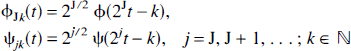
\begin{array}{l} ϕ_{J_{k}} (t) & = & 2^{J / 2} ϕ (2^{J} t - k), \\ ψ_{j k} (t) & = & 2^{j / 2} ψ (2^{j} t - k), j = J, J + 1, \dots; k \in N \end{array}

(2)

for some fixed positive J. A function f ∈ L²(ℝ) may be expanded in a wavelet base as:

f (t) = \sum_{j = J}^{\infty} \sum_{k \in N} d_{j k} ψ_{j k} (t) + \sum_{k \in N} c_{J k} ϕ_{J k} (t)

(3)

where d_jk = 〈f, ψ_jk〉, c_Jk = 〈f, ϕ_Jk〉, and 〈•〉 is the standard L²-inner product of two real functions. The wavelet function represents the frequency contents of f(t) near 2^j localized to data positions k2^−j, whereas the scaling function represents the residual term of the expansion up to resolution J. In contrast to standard Fourier sine and cosine series, the structure of wavelets means that they may be localized via dilation in the frequency domain and via translation in the data domain. This localization allows parsimonious representation for a wide set of functional spaces (Donoho, 1993).

In the case of ET images, major interest resides in bases of smooth wavelets that can provide suitable representation of patterns of measured radioactivity (Ruttiman et al., 1996; Turkheimer et al., 1999). Orthonormal bases of cubic-spline wavelets, also known as Battle-Lemarie wavelets (Battle, 1987; Lemarie, 1988), are the common choice for this particular application because they provide the optimality conditions that guarantee the result of Eq. 1 (Ruttiman et al., 1996; Turkheimer et al., 1999).

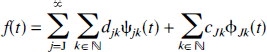
The DWT algorithm is illustrated in Fig. 2. It consists of iterative steps, each made by the application of two complementary low- and high-pass filters (identified by L and H, respectively) and subsequent dyadic decimation (Mallat, 1989). The wavelet coefficients are the output of the high-pass operation, whereas the coefficients of the scaling function are obtained from L. By application of L and H on the latter coefficients, one obtains the wavelet and scaling coefficients for the next resolution.

FIG. 2.

The discrete wavelet transform is obtained by applying complementary low-pass and high-pass filters and subsequent decimation (H and L). Both H and L are applied to data vector x₁, x₂, …, x₈. The output of H is the four wavelet coefficients for the first resolution; the output of L is the four coefficients of the scaling function. The wavelet coefficients of the other resolution levels are obtained by iterating the low- and high-pass filtering steps on the coefficients of the scaling function.

The DWT can be easily extended to two or more dimensions. In the case of an image (Fig. 3), filters with subsequent decimation are applied independently to rows and columns to produce three quadrants of wavelet coefficients H, V, D (labeled horizontal, vertical, and diagonal, respectively) and the quadrant C of scaling coefficients. As in the one-dimensional case, the iteration of the filtering and decimation steps on quadrant C produces the wavelet and scaling quadrants for the next resolution level.

FIG. 3.

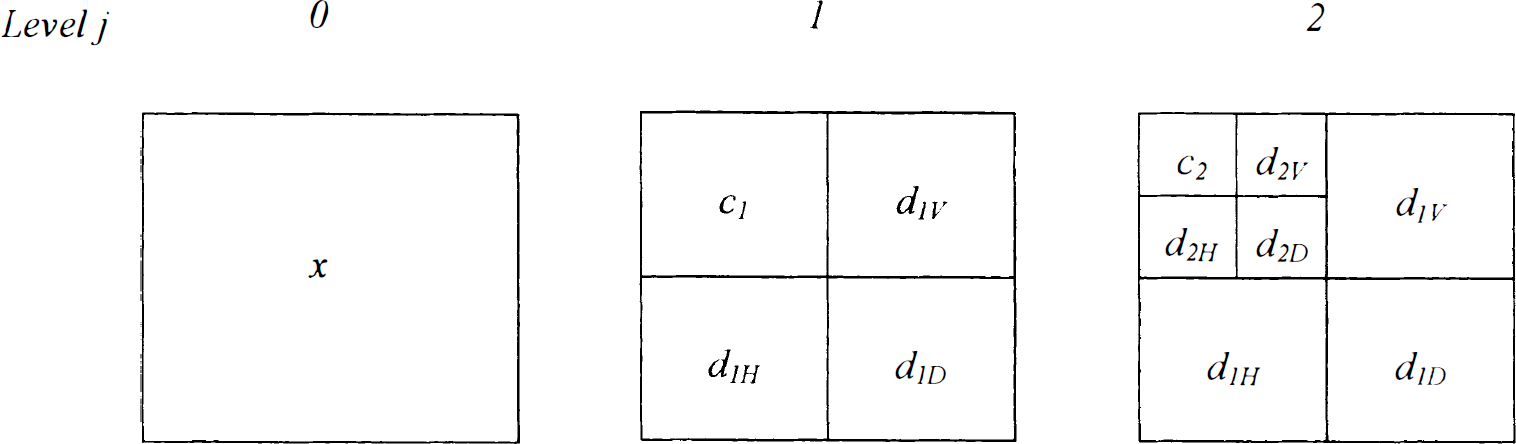
The two-dimensional wavelet transform. The transform is performed on images by applying the filters L and H to rows and columns. This operation produces a quadrant c containing the coefficients of the scaling functions and three quadrants of wavelet coefficients d usually labeled as horizontal, vertical, and diagonal (H, V, D). Wavelet coefficients of higher resolution are obtained by applying the above filtering steps to quadrants c.

TRANSLATION-INVARIANT DISCRETE WAVELET TRANSFORM

The DWT does not enjoy the translation-invariant property; its representation across resolution levels may change substantially after a shift of the signal in the data domain (Coifman and Donoho, 1995). This means that the representation of the signal is dependent on its alignment with the kernel of wavelet functions. If the signal is aligned, then its representation may be made of few coefficients on different resolution levels. Instead, if the same signal is shifted, its alignment with the wavelet base may be lost and the subsequent transform will produce a wavelet representation that will not be sparse anymore, and the number of its wavelet coefficients will increase with a correspondent decrease of their magnitude, often under the noise level (Coifman and Donoho, 1995). In the case of sparse signals with high noise levels, application of the DWT results in artifacts and loss of detection power (Turkheimer et al., 1999).

The lack of translation invariance is a consequence of the violation of the Nyquist principle caused by the dyadic decimation (Simoncelli et al., 1992). The decimation step is needed to guarantee the orthogonality of the representation, but it causes the undersampling of the output of the two filters H and L(Simoncelli et al., 1992). In fact, taking one out of two samples is adequate only in the case of perfect sync filters, which are not the type used by the DWT.

Coifman and Donoho (1995) introduced DWT-TI, which produces a translation-invariant representation of the signal with a minimal increase of complexity. This approach was further extended to two and n dimensions (Turkheimer et al., 1999). The resulting set of the DWT-TI wavelet coefficients is overcomplete and therefore does not imply a unique inverse transform. The approach of Coifman and Donoho (1995) constructs a unique inverse by averaging all reconstructions obtained by all shifted DWTs. However, other approaches are available-for instance, the one of Nason and Silverman (1995) is based on choosing the “best” shifted DWT among all present in the DWT-TI.

When applied to ET images, the DWT-TI was able to eliminate the artifacts in the reconstruction that are typical of the traditional DWT (Turkheimer et al., 1999). Therefore, in the procedure in Fig. 1, the WT and its inverse are intended to be performed through DWT-TI algorithms.

KINETIC MODELING IN THE WAVELET DOMAIN

The estimation procedure in Fig. 1 requires the kinetic modeling of the time course of wavelet and scaling coefficients. Conceptually, this step is quite different from the usual pixel-by-pixel approach. A pixel is the sampling unit of the digitized image and does not necessarily have any relation with the underlying measured pattern. A wavelet coefficient instead represents a spatial object of a certain scale in a certain position. More interestingly, if a wavelet coefficient is consistently in the same scale and location through sampling times t_i = t₁, t₂, …, t_M, then the spatial object it represents is kinetically homogeneous. This stems from the obvious fact that if a spatial object were made of components with different kinetics, then its spatial frequency would change through time and hence its wavelet representation. Therefore, modeling in the wavelet domain implies the application of the estimation process to spatial patterns with homogeneous kinetics; because the DWT is a linear operator, these kinetics will be the same in wavelet space as in image space.

The above setting suggests that any linear modeling procedure, consistent with the underlying biology, may be used as estimation operator κ(•), and that κ(•) is the same estimation procedure whether it is applied in image space or wavelet space.

The most common approaches to the analysis of PET-SPECT studies have been based on compartmental models (Carson, 1986; Cunningham and Lammertsma, 1994). For these models, estimation procedures mainly rely on classic results on nonlinear regression and least-squares theory (Carson, 1986). Given that e(w,t₁), e(w,t₂), …, e(w,t_M) are white noise processes, it is then straightforward to obtain not only the estimates σ̂_wt(w) but also their statistical uncertainty in terms of the correspondent σ̂_wt(w) (Bates and Watts, 1988).

When a tracer is well characterized, the nonlinear estimation procedure may be simplified to a linear fit applied to a reduced set of data points (Gjedde, 1981; Logan et al., 1990, 1996; Patlak et al., 1983; Patlak and Blasberg, 1985). Linear methods are appealing for their computational speed and inherent ability to converge with high noise levels (Carson, 1993). They are also less sensitive to the problem of tissue heterogeneity (Carson, 1993), which is relevant in this context given the need for modeling data at different resolutions; these methods will be used in the application section of this article.

For all other modeling approaches to PET and SPECT, the reader is referred to the literature (Carson et al., 1998; Lawson, 1999; Myers et al., 1996).

Finally, it is relevant to consider that the space-time modeling approach in Fig. 1 may be extended beyond quantitative approaches. In nuclear medicine, the functional κ(•) may be generalized as a data-reduction operator that uses the temporal distribution of the tracer to classify the pixels of an image according to their kinetic behavior (Lawson, 1999). The functional forms of the kinetics of interest may not even be obtained from a physiologic model, but, for example, they may be extracted from the data themselves as eigenvectors from a PCA of the dynamic data set (Barber, 1980). In the case of PCA, κ(•) projects the time course of each pixel on a selected eigenvector of the data set Y(s,t_i) and provides a score that quantifies how much of that kinetic is expressed in that pixel. Pixels with similar kinetics may then have similar scores, and PCA may be used to identify regions of interest (ROIs) with homogeneous kinetic behavior. Because data are corrupted by noise, some spatial modeling may be needed to improve ROI extraction. Therefore, the procedure in Fig. 1 may be applied to estimate the pattern of linear scores P(s) for the eigenvector of interest. An example of such an application will be illustrated on a dynamic SPECT data set.

STATISTICAL THRESHOLDING OF WAVELET COEFFICIENTS

The final step of the procedure in Fig. 1, before reconstruction, amounts to the thresholding of the wavelet coefficients P̂_wt(w_x,w_y). Given that e(w,t₁), e(w,t₂), …, e(w,t_M) are white noise processes and that the application of κ(•) amounts to a least-squares procedure, than we can assume that

{\overset{\circ}{P}}_{wt} (w) = P_{wt} (w) + e (w)

(4)

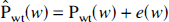
where P_wt(w) is the DWT of P(s) and e(w) are independent normal scores normally distributed with mean 0 and estimated standard error σ̂_wt(w)-that is, e(w) ∼ N(0, σ̂_wt(w))-and N 0 is the normal probability distribution function.

The sparseness of the wavelet expansion makes it reasonable to assume that essentially only a few “large” P̂_wt(w) contain information about the underlying function P(s), whereas “small” P̂_wt(w) can be attributed to the noise that uniformly contaminates all coefficients (Turkheimer et al. 1999).

Donoho and Johnstone (1994, 1995) suggested the extraction of significant coefficients by nonlinear thresholding in which wavelet coefficients are set to 0 if they are below a certain threshold level λ. Two standard thresholding policies are “hard” thresholding

{\overset{\circ}{P}}_{wt}^{*} (w) = {\overset{\circ}{P}}_{wt} (w) * I (| {\overset{\circ}{P}}_{wt} (w) | > λ * {\overset{\circ}{σ}}_{wt} (w)),

(5a)

and “soft” thresholding

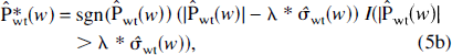
\begin{array}{l} {\overset{\circ}{P}}_{wt}^{*} (w) & = & sgn ({\overset{\circ}{P}}_{wt} (w)) (| {\overset{\circ}{P}}_{wt} (w) | - λ * {\overset{\circ}{σ}}_{wt} (w)) I (| {\overset{\circ}{P}}_{wt} (w) | \\ > λ * {\overset{\circ}{σ}}_{wt} (w)), \end{array}

(5b)

where I(•) is the indicator function and the superscript asterisk indicates the filtered coefficients.

Hard thresholding is a “keep” or “kill” rule that has the property of producing small bias but larger variance as a result of the brisk separation between noise and signal (Donoho and Johnstone, 1994, 1995), although this is less of a problem if the translation-invariant approach is adopted (Lang et al., 1996). Soft thresholding is a “shrink” or “kill” rule that reduces the variance from such artifacts at the cost of an increase in bias, because the coefficients are all reduced by an amount equal to λ (Donoho and Johnstone, 1994, 1995). Previous results (Turkheimer et al., 1999) suggest that the use of hard thresholding combined with the DWT-TI achieves minimal bias and substantial reduction of artifacts in PET images, and therefore it will be the policy of choice for the application section of this article.

The selection of an appropriate threshold λ is a more difficult problem, because the results used by Turkheimer et al. (1999) are tenable only with the strong assumption of homogeneous variance (i.e., stationarity) in the data domain. However, the availability of estimates σ̂_wt(w) allows the relaxation of the stationarity constraint on the noise model. In fact, the most intuitive approach is now to adopt a model of pointwise stationarity and, accordingly, to use each σ̂_wt(w) as the estimate of the error of each wavelet coefficient.

However, as shown below, pointwise estimates of the wavelet variance may not be accurate enough, particularly at the finest resolution that is the most sensitive to deviations from normality (Vidakovic, 1999). In this case it may be of interest to consider “locally stationary” processes. These are noise processes whose spectral behavior varies smoothly in the data domain. Technically, a Gaussian noise process is “locally stationary” under mild conditions, the most important being that its noise spectrum (i.e., the Fourier transform of its autocorrelation function) is of bounded total variation and continuously differentiable in both frequency and data domain (Dahlhaus, 1997; Neumann and von Sachs, 1997). The model of “locally stationary” process suits particularly well the noise characteristics of PET and SPECT images. General considerations of the physical and physiologic factors involved in the measurement suggest that the error variance is spatially smooth and possibly constant within a small neighborhood of pixels (Holmes et al., 1996). Therefore, if one considers the model of local stationarity valid for the ET study under analysis, a local pooling of estimates σ̂_wt(w) may be used to reduce their variability.

Interestingly, for both the models of pointwise and of local stationarity, the optimal rate of the least-squares risk of Eq. 1 is attained at any threshold λ^J that satisfies (von Sachs and MacGibbon, 1998):

\sqrt{2 log # ({\overset{\circ}{P}}_{wt}^{J} (w))} \leq λ^{J} \leq \sqrt{2 log # ({\overset{\circ}{P}}_{wt} (w))}

(6)

where J labels the resolution level and the operator #(•) indicates the number of nonnull elements in the set. In other words, the optimal rate of Eq. 1 is obtained by use of the so-called universal threshold (Donoho and Johnstone, 1994, 1995) applied to the entire set of wavelet coefficients or separately on each resolution level. The universal threshold approaches the optimization problem of Eq. 1 from a minimax point of view, and therefore it tends to produce an oversmoothed solution (Turkheimer et al., 1999); for this reason, the use of the levelwise threshold is preferred (von Sachs and MacGibbon, 1998).

Alternatively, one may turn to the levelwise application of Stein's unbiased risk estimator, better known as SURE (Donoho and Johnstone, 1995). The application of this estimator was described in detail previously (Turkheimer et al., 1999). SURE produces a solution with better least-squares properties, at least asymptotically, and was proved suitable also for the locally stationary case (von Sachs and MacGibbon, 1998).

METHODS

The estimation scheme in Fig. 1 was applied to simulated data and dynamic studies acquired with ET scanners. An artificial data set was used to explore the performance of thresholding policies in simulated conditions that resembled ET dynamic scans. For numeric studies of wavelet filters in the one-dimensional case, the reader is referred to von Sachs and MacGibbon (1998).

The first application to real data considers two dynamic PET studies with FDG and [¹¹C]raclopride. The aim was to evaluate whether wavelet filters recovered the underlying patterns of glucose metabolism and dopamine receptor density, patterns that are well known in the normal brain. The next application involved the investigation of the unknown pattern of distribution of the inflammation marker [¹¹C](R)-PK11195 in a pathologic brain. This tracer is particularly suitable for testing the validity of the estimation approach because of the low signal-to-noise ratio in the images. Finally, the methodology was used to recover ROIs with homogeneous kinetic behavior from a dynamic SPECT study of dopamine receptors in the brain. Here the objective was merely illustrative: it underlines the generality of the estimation approach that may incorporate various approaches to the modeling of the signal in the time dimension.

Details on acquisition and kinetic analysis will be given in the following sections for each experiment. The software used was written in MATLAB (The Mathworks Inc., Natick, MA, U.S.A.) and run on an Ultra-Sparc 1 (143-MHz CPU) Sun Workstation (SunSystems, Mountain View, CA, U.S.A.). The DWT was implemented as detailed in Turkheimer et al. (1999). The two-dimensional DWT in its translation-invariant form was used for the analysis of all studies.

A linear estimation procedure was used to estimate the kinetic parameter of interest in all examples. In applications to real data sets, unweighted linear least-squares was preferred to the weighted procedure. This choice stems from the difficulty in obtaining consistent estimates of the variance for the wavelet coefficients W(w,t_i); errors in the determination of weights may neutralize any benefit generated by the use of a weighted procedure or may introduce bias into the estimates (Carson, 1993). The time windows for the application of the linear modeling operators were selected by previous verification that plots for some ROI data showed linear behavior.

In all studies, unless otherwise specified, the wavelet coefficients corresponding to the background were set to 0. This step is important to retain the efficiency of data-dependent thresholds of the SURE and to avoid unnecessarily conservative corrections for universal thresholds that depend on the total number of nonnull wavelet coefficients in the image.

Following the theoretical framework noted above, a pooling procedure for error estimates σ̂_wt(w) was also introduced for evaluation; estimates σ̂_wt(w) were pooled by averaging their values on a 3 × 3 neighborhood only at the finest resolution level.

Synthetic dynamic study

A simulation study was devised to investigate the property of the estimation procedure with attention to the performance of the SURE and universal thresholds. We wanted to reproduce patterns of different scale in nonstationary noise conditions that resembled the ones of ET scanners.

One synthetic image (128 × 128) was generated that contained a uniform background of value equal to unity, to which four circles were added (radius 4, 8, 16, and 24 pixels). Height of the signal was 1. This image, A(x,y), represented the pattern that had to be recovered from the dynamic study. The dynamic set V(x,y,t) was then generated that reproduced the simple kinetic:

V (x, y, t) = A (x, y) • \int_{0}^{t} Cp (t) d t,

(7)

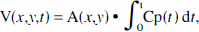
where Cp(t) is a simulated blood time course from a bolus injection. This equation describes a simple irreversible trapping of a tracer in a body compartment according to the distribution pattern A(x,y).

White noise was added with standard deviation proportional to the values V(x,y,t) to create the nonstationary noise field. In fact, given the linear relation between A(x,y) and V(x,y,t), the noise variance is proportional to the values of the pattern. To recreate the low signal-to-noise ratios of ET images, the proportionality constant was set equal to the background value (i.e., 1). All images of the dynamic sequence were then smoothed with a Gaussian filter of full width at half maximum = 4 pixels.

Because the pattern of the signal was smooth and the noise was proportional to it, this data set reproduced a locally stationary noise field as defined by Dahlhaus (1997). The data set contained 10 dynamic frames to simulate the conditions of the real data sets contained in the application section of this article.

The estimation procedure in Fig. 1 was then applied. The operator κ(•) consisted of a weighted linear least-square procedure where the known noise variances were used as weights: correspondent uncertainties of estimates were obtained by use of classic results for linear regression. Both the SURE and the levelwise universal thresholds (left side of Eq. 6) were used.

FDG dynamic study

A dynamic FDG study of brain function was considered. This case was of interest because it allowed an evaluation of the denoising properties of the methodology on a well-known pattern of distribution, as well as of its ability to preserve fine structural details of the image. Dynamic frames were acquired with an ECAT 953B PET camera (CTI/Siemens, Knoxville, TN, U.S.A.). Measurements of the arterial blood concentration of the tracer were also available. Metabolic rates for FDG were estimated by use of the Patlak plot (Gjedde, 1981; Patlak et al., 1983; Patlak and Blasberg, 1985). The data points in the time interval of 20 to 60 minutes after injection were used (nine frames) for the linear estimation. Only the levelwise universal threshold was used.

[¹¹C]raclopride dynamic study

The second example considered a dynamic [¹¹C]raclopride study of the D2-receptor distribution in the normal brain. Frames were acquired with an ECAT 953B PET camera (CTI/Siemens). Arterial samples were not available, and a reference region placed on the cerebellum was used as input function.

Estimates of the distribution volume ratio (DVR) were obtained with the Logan plot (Logan et al., 1996). The original equation of this plot reads:

\int_{0}^{t} C_{i} (t) d t / C_{i} (t) = DVR \int_{0}^{t} C_{ref} (t) d t / C_{i} (t) + c,

(8a)

where C_i(t) is the tissue time activity, C_ref(t) is the time activity in the reference region that is assumed to be devoid of D2-receptors, and c is a constant. Although C_ref(t) can be assumed noise-free as being sampled on a large ROI, the same cannot be said for the term C_i(t), which appears on both sides of the linear equation. However, Carson (1993) showed that the simple rearrangement of Eq. 8a as

C_{i} (t) = - (DVR / c) \int_{0}^{t} C_{ref} (t) d t + (1 / c) \int_{0}^{t} C_{i} (t) d t,

(8b)

substantially reduces the bias of the estimated parameters even with noise levels typical of pixels' time courses and allows the use of the Cramer-Rao lower bound (Beck and Arnold, 1977) to estimate the standard deviation of the parameters. The frames for the time interval 5 to 60 minutes (nine frames) were used for the linear estimation of DVR using (6b) after previous verification that the plot of Eq. 8a showed linear behavior in this time window. The levelwise universal threshold was used for the thresholding of wavelet coefficients.

[¹¹C](R)-PK11195 dynamic study

The ligand [¹¹C](R)-PK11195 binds to the peripheral benzodiazepine binding site (Banati et al., 1997; Banati and Myers, 1997; Benavides et al., 1988), and in normal healthy brain tissue binding is minimal (Banati et al., 1997). However, in stroke (Ramsay et al., 1992) and inflammatory (Banati et al., 1999) as well as neurodegenerative brain disease, the binding site is highly expressed by activated microglia and brain macrophages. Here, a dynamic study of a patient with herpes encephalitis, an inflammatory process that is largely confined to structures of the limbic system, sparing for instance the cerebellum, was used for analysis. The scan was performed on an ECAT 953B PET camera (CTI/Siemens) after bolus injection of 386 MBq single enantiomer [¹¹C](R)-PK11195 (specific activity 45.5 GBq/mmol). Dynamic data were collected over 60 minutes in 17 time frames. Kinetic analysis was performed with the Logan plot (Logan et al., 1996) as detailed above. The frames of the time interval 5 to 60 minutes (10 frames) were used for the analysis, and the time course of a reference region placed on the cerebellum was used as input function. Wavelet analysis was performed with the levelwise universal filter.

[¹²³I]epidepride SPECT dynamic study

The SPECT images were acquired using the high-affinity D2/D3 receptor ligand epidepride labeled with ¹²³I. In vivo, SPECT studies of the brain in healthy volunteers with [¹²³I]epidepride visualize D2/D3 receptor binding in the striatum, thalamus, temporal cortex, and amygdala (Kessler et al., 1992). After the injection of 180 MBq [¹²³I]epidepride, projection data were acquired using the PICKER-3000XP triple-headed gamma camera and fan-beam collimators (Picker International Inc, Cleveland, OH, U.S.A.). Two imaging sessions were carried out between 0 and 120 minutes (16 frames) and 187 and 309 minutes (10 frames) after injection. Images were corrected for uniform attenuation using an ellipse fitted on a slice-by-slice basis. Individual time frames were realigned to allow the use of the same set of volumes of interest to be applied on all time frames acquired.

PCA was performed on the entire volume of 28 frames (Barber, 1980), and only the eigenvectors accounting for 99% of the variance were retained. As previously explained, the aim of the kinetic analysis was to detect regions of the brain with homogeneous kinetic behavior. In image space, such segmentation was obtained by projecting each pixel time course on the retained eigenvectors and obtaining images of pixel weights. Weights and their standard deviations were obtained by linear least-squares.

In wavelet space, the same computation was performed on each wavelet time course. Wavelet shrinkage was performed with the levelwise universal threshold. Because this application was intended as an exercise of automatic ROI extraction, the wavelets corresponding to the background were not suppressed, as in previous examples.

RESULTS

Synthetic dynamic study

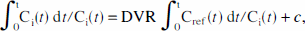
Figure 4 shows the raw data and the results of the experiment. Figure 4A shows the original pattern of the parameter that generated the synthetic dynamic study. Figure 4B displays the results of the estimation of the pattern obtained by kinetic analysis without the use of spatial modeling. Figures 4C and 4D contain the patterns estimated with the use of wavelets. Figure 4C shows the results obtained with the levelwise universal filter. The image appears completely denoised and the pattern is recovered with the exception of the smallest structure. This was expected because this structure had height equal to the noise level and width equal to the smoothing kernel. These results resemble the ones obtained previously with stationary noise conditions (Turkheimer et al., 1999).

FIG. 4.

Data and results for the synthetic dynamic data experiment. (A) The original pattern that generated the simulated dynamic scan of the form V(x,y,t) = A(x,y) • ∫^t_o Cp(t) dt where A(x,y) is the pattern in the panel and Cp(t) is a simulated input function. A nonstationary noise field was then added to the dynamic set V(x,y,t). The noisy data sets was first analyzed by application of pixel-by-pixel linear regression without spatial modeling; B shows the resulting pattern. Data were then analyzed through the time-space modeling procedure described in the text. The pattern in C is the one recovered with the levelwise universal filter. (D) The output of the Stein's unbiased risk estimator (SURE) filter.

Figure 4D illustrates the image obtained with the SURE filter. Although some noise reduction is apparent, the results with the filter do not match those obtained with the analogous pattern and stationary noise conditions (Turkheimer et al., 1999). This result stems from the low number of degrees of freedom (9 from the 10 frames dynamic) of the estimates σ̂_wt(w). Because the SURE filter is derived from an estimation procedure specifically designed for multivariate normal distributions (Turkheimer et al., 1999), 20 or more degrees of freedom are needed for the filter to work effectively. For this reason, this filter was not considered for our other studies.

The application of the variance-pooling procedure produced no appreciable difference for both filters (data not shown). With the universal filter, the final image is already smooth and can be hardly improved by better variance estimates in the finest resolution. In the case of the SURE, improvement in this resolution cannot be visible, given the inability of the filter to deal with the nonnormality of the coefficients at all resolution levels.

FDG dynamic study

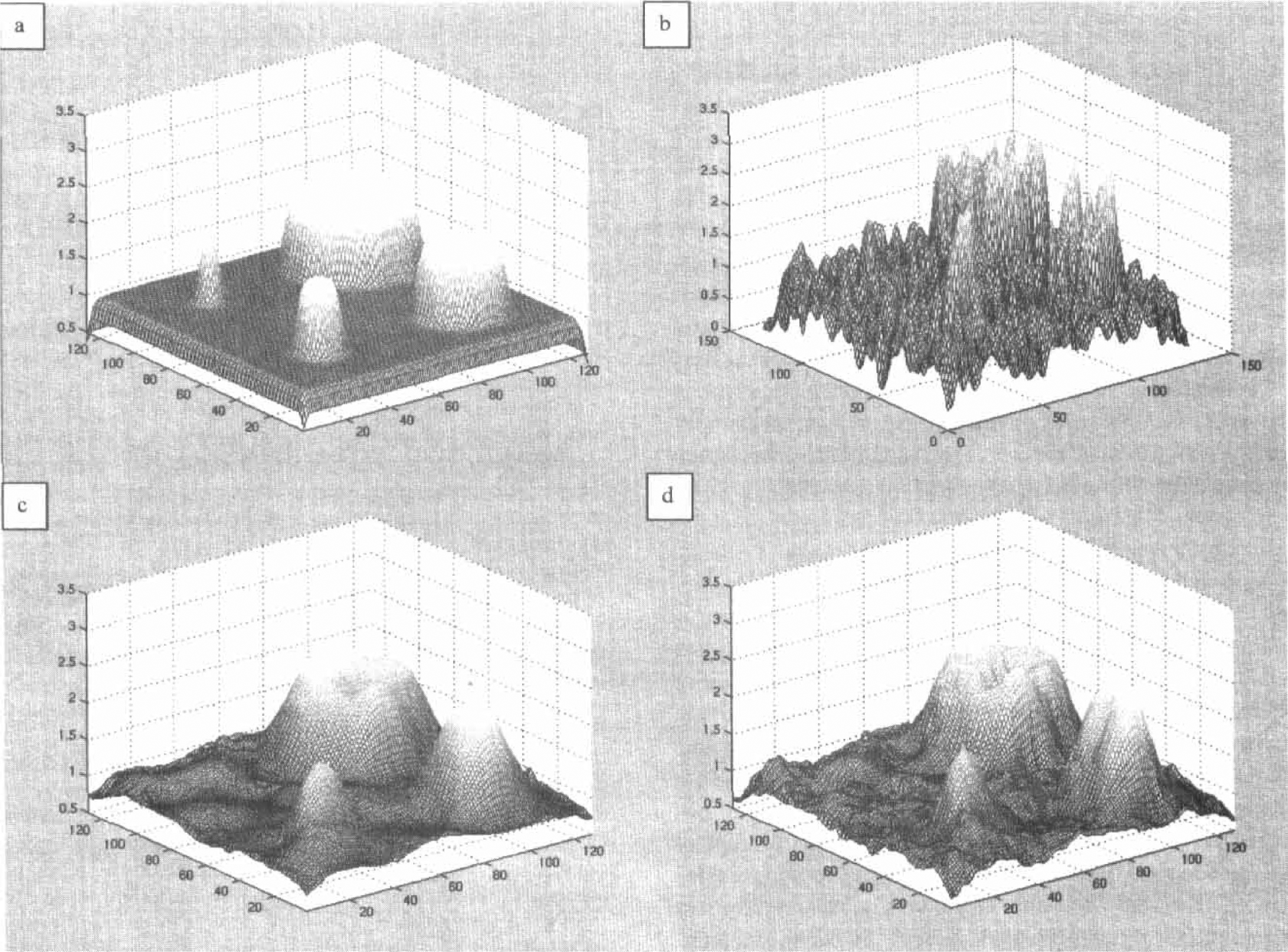
Figure 5 illustrates the parametric maps of two transaxial sections with and without spatial modeling. Figures 5A and 5B show the results of the application of the Patlak plot to the dynamic data. The results of the application of the wavelet methodology are shown in the lower panels. Figures 5C and 5D show the results obtained by application of the time-spatial modeling procedure for the corresponding two sections; the images are mostly denoised, and the structure of the striatum and the thalamus and the fine details of the cortical structures are preserved. However, these images still contain some artifacts that appear as spurious dots. These artifacts are due to the low degrees of freedom of estimates σ̂_wt(w) (seven from the nine frames used in the Patlak plot) at the finest resolution. Local pooling of these estimates removed these artifacts almost entirely, as shown in Figs. 5E and 5F.

FIG. 5.

Results of the application of a standard modeling procedure to a dynamic [¹⁸F]fluorodeoxyglucose (FDG) study of brain metabolism with and without spatial modeling. (A, B) Parametric maps of FDG metabolic rates (mL/g per minute) of two transaxial sections obtained by application of the Patlak plot to the dynamic frames. (C, D) Corresponding slices obtained by the wavelet estimation procedure. With this methodology, the Patlak plot was performed on the wavelet transforms of the dynamic frames; the resulting wavelet parametric maps were then filtered and back-projected. (E, F) Results of the same procedure when a local smoothing of wavelet variances at the finest level was added, before filtering, to reduce artifacts.

[¹¹C]raclopride dynamic study

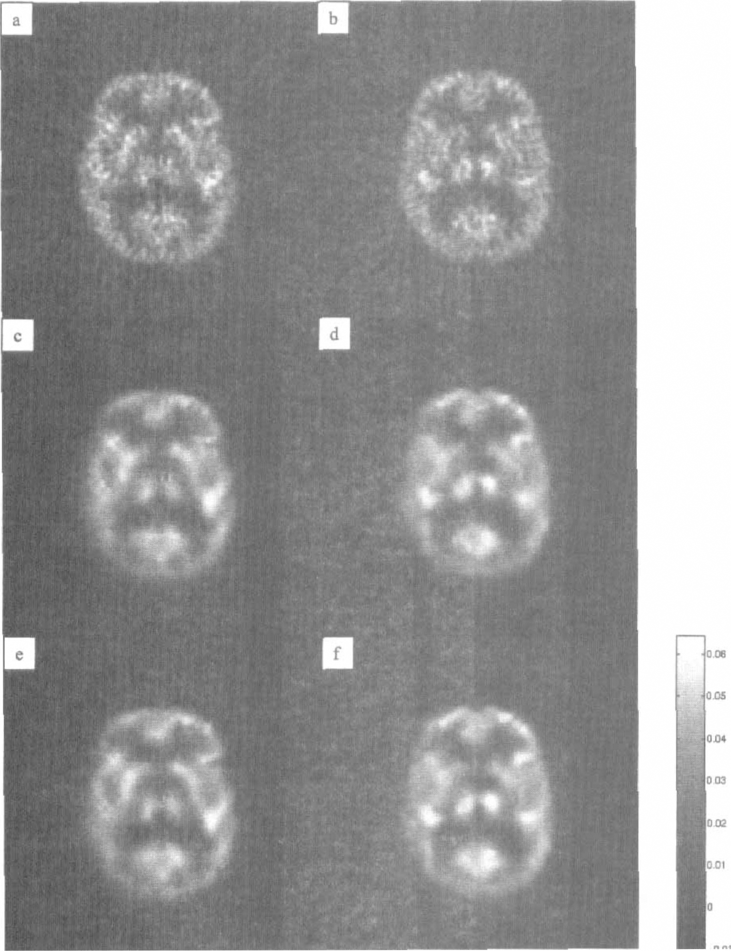
Figure 6 illustrates the results of the direct application of the Logan plot to the sequence of scans for two transaxial sections. The familiar shape of the striatum is visible but the parametric maps are corrupted by high levels of noise. This noise is completely removed by the wavelet procedure, as illustrated in Figs. 6C and 6D. The parametric image appears homogeneously smoothed, but the caudate and putamen retain their fine scale structure. The application of the pooling procedure for wavelet variances produced no appreciable differences (data not shown); this may be expected given the absence of artifacts in the reconstructed images.

FIG. 6.

The wavelet procedure was also applied to a dynamic positron emission tomographic study with [¹¹C]raclopride of the D2-receptor density in the normal brain. (A, B) Parametric maps of distribution volume ratio (DVR) obtained with the Logan plot for two transaxial sections that contain the striatum. (C, D) Corresponding slices obtained with the wavelet procedure.

[¹¹C](R)-PK11195 dynamic study

Herpes encephalitis typically affects the limbic system, leading to nerve cell death and massive activation of microglia in the area of damage. Figure 7 illustrates the parametric map of DVR for PK11195 superimposed on the corresponding magnetic resonance image (Fig. 7A) plus the one obtained with wavelet filtering (Fig. 7B). In this patient, a left-sided herpes encephalitis led to a severe neuroinflammatory response with activation of microglia throughout the limbic system (Banati et al., 1999). The parametric map (see Fig. 7A) shows an extended pattern of signal, particularly prominent in the left hippocampal formation, left temporal lobe, and left and right anterior insular cortex. However, the high level of noise makes the interpretation of the image difficult, particularly if, as in the case of the limbic system, a distributed neural network is affected and signals in other areas, such as the densely interconnected frontal lobe, are expected.

FIG. 7.

(A) Parametric image of [¹¹C](R)-PK11195 binding. In this patient, a left-sided herpes encephalitis has led to a neuroinflammation and consequent activation of microglia in the left hippocampus (HC), the temporal lobe (TL), and the ipsilateral and contralateral insula (INS). (B) Wavelet filtering preserves this pattern and reveals a left frontal signal consistent with the severe aphasia observed clinically in this patient.

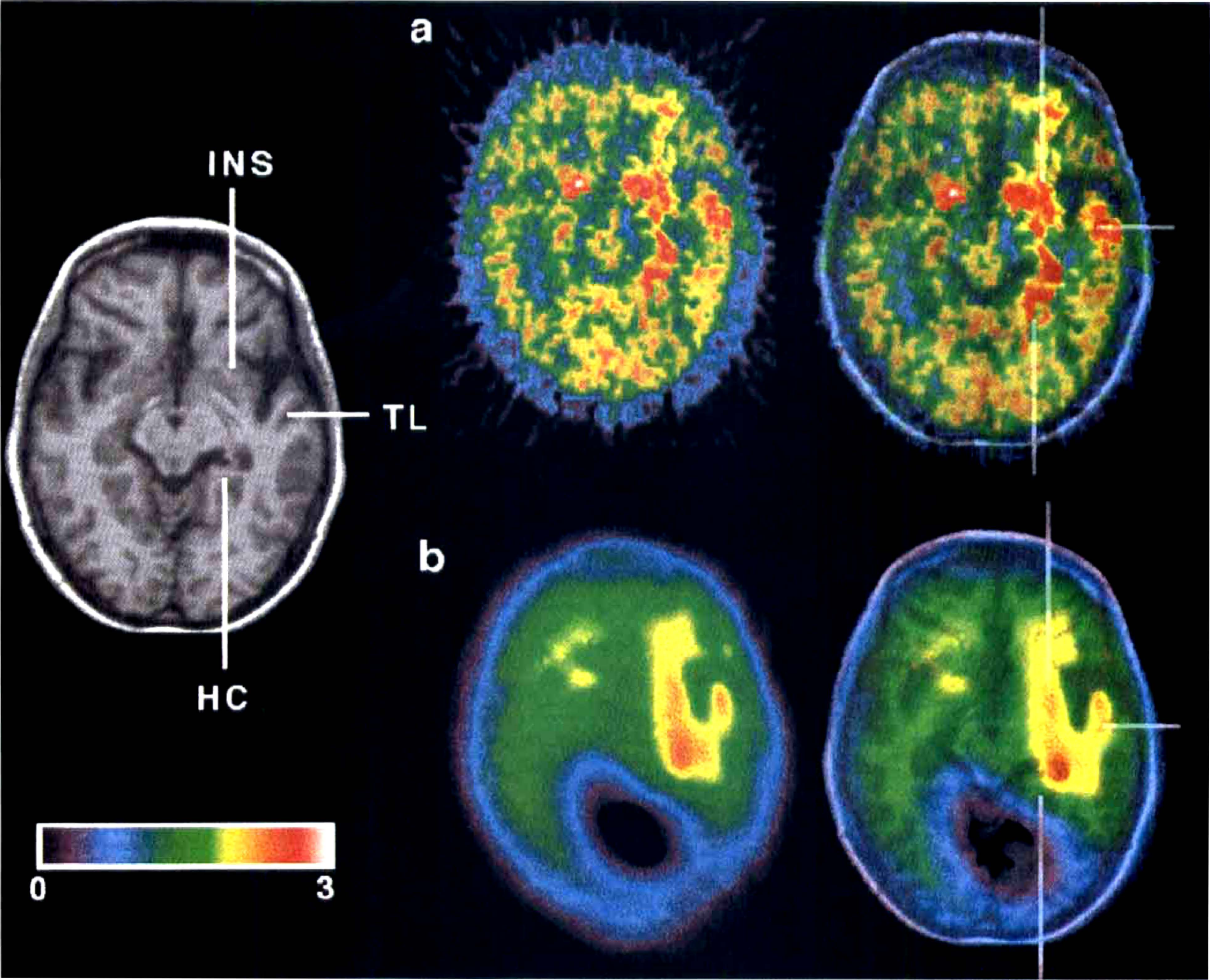
The wavelet-treated image (see Fig. 7B) is heavily smoothed because of the high noise level but clearly shows the described pattern of left hippocampal, left temporal, and insular signal. In addition, the expected involvement of the anatomically connected left frontal lobe can now be detected as an increase in PK binding; such a finding is implicated by the severe aphasia observed clinically in this patient and was also observed more clearly in patients of the same group (Banati et al., 1999).

In contrast, all the posterior signal, particularly the one seen in the area of the confluent venous sinus in the parametric map that is unrelated to the pathology, can no longer be seen in the wavelet-treated image. Inspection of the local properties of DVR in this area showed that standard errors of the estimates were quite high because of the vascular origin of the signal. Therefore, wavelets corresponding to this signal were suppressed in the thresholding process.

[¹²³I]epidepride SPECT dynamic study

From the PCA of the SPECT study, two eigenvectors were selected that accounted for 99% of the variance of the dynamic volume. The first eigenvector represents the average uptake of the tracer in the receptor regions, the striatum and temporal cortex (data not shown). The second eigenvector (Fig. 8A) differentiates between the striatal areas, which have higher uptake, and the cortical ones. The image of the pixel weights for this eigenvector is shown in Fig. 8B for one transaxial section selected at the level of the basal ganglia.

FIG. 8.

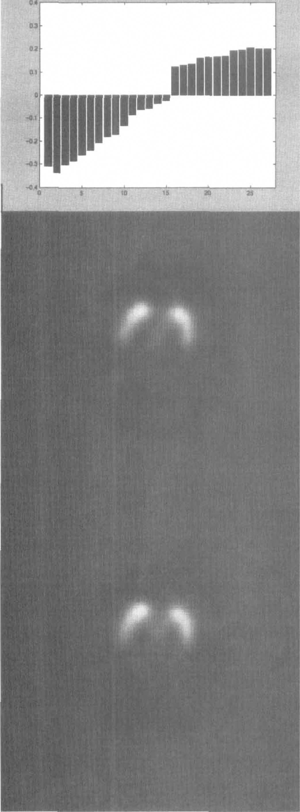
Data and results for the analysis of a single photon emission computed tomographic dynamic study of D2 dopamine receptor density in the brain. The kinetic analysis was performed through principal component analysis. (A) The eigenvector that differentiates between regions with higher receptor density (striatum) and the ones with lower density (temporal cortex). (B) The pixel weights for this eigenvector for one transaxial slice at the striatum level. (C) The same image, but computed with the wavelet procedure. The pattern of the basal ganglia is preserved, but noise in the brain and in the background is smoothed away.

Figure 8C displays the same image when PCA was performed in the wavelet domain; wavelet filtering improves the regions' definition by recovering the striatal pattern of the eigenvector while removing the background noise. Figure 9 shows the entire pixel weight maps with and without wavelet filtering.

FIG. 9.

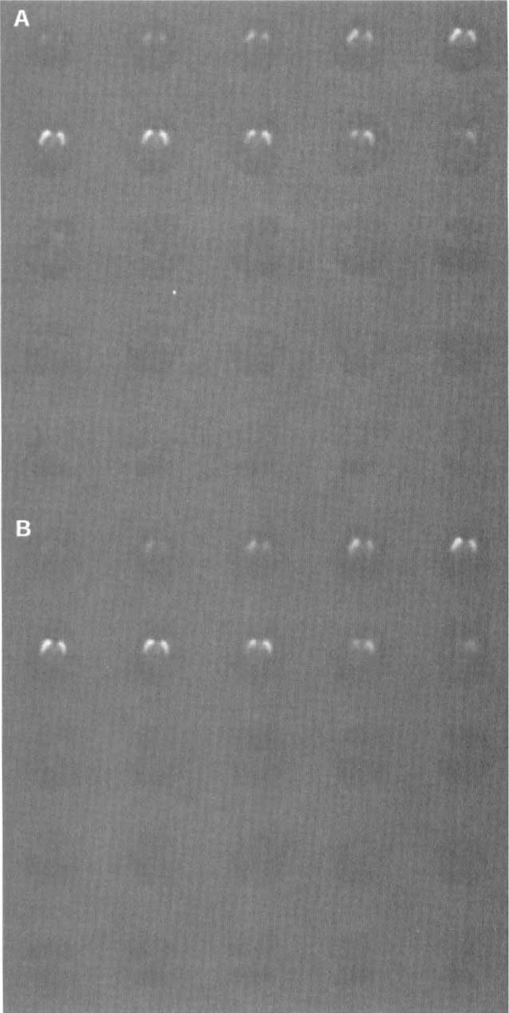
The whole data set of the single photon emission computed tomographic study of Fig. 8. (A) Pixel weights map. (B) The same map estimated through the wavelet procedure.

DISCUSSION

This article introduces a new procedure that allows the combined kinetic and spatial modeling of dynamic PET-SPECT studies. With this methodology, parametric maps are obtained by performing the kinetic modeling and statistical analysis on the wavelet transforms of the dynamic scans.

Theory and algorithms were developed to allow the use of linear modeling operators. However, a pragmatic extension of the framework to nonlinear operators may be also considered, because in PET deviation of lincarity is usually mild. For example, nonlinear modeling operators applied in sinogram space (Meikle et al., 1998) produced little bias in the parameters. Such bias should therefore be reduced in wavelet space because wavelet coefficients represent a local expansion of the image, whereas a coefficient in sinogram space represents data in a line of coincidence crossing the entire field of view. However, no general rule can be given, and appropriate validation should be considered for each operator in any single protocol.

The statistical setting allows the relaxation of constraints on the noise processes that were embedded in previous work, and it is now suitable to deal with nonstationary noise conditions under very mild assumptions.

Two wavelet filters that are standard in wavelet literature were tested, the universal and the SURE. The results on synthetic and real data confirm that the universal filter is very efficient in removing noise while preserving the structures of parametric images to their finest detail. Application to FDG and raclopride dynamic studies positively tested the ability of the filter to recover the familiar patterns of distribution of the two tracers. The case of a [¹¹C](R)-PK11195 dynamic study illustrated its usefulness in the interpretation of images when little was known a priori of the tracer's distribution and noise levels were high. This example also emphasized the ability of wavelets to perform multiresolution analysis that considers the noise properties locally. In contrast, the SURE filter has shown poor performance in such applications; this filter has known limitations because of its lack of robustness (Neumann and von Sachs, 1995) and should be applied only to noise processes that are purely Gaussian. A pooling procedure for wavelet variances was also introduced and proved to be effective in removing wavelet artifacts that may appear in the reconstructed images as a result of the poor statistical properties of the estimates.

Although the results of a standard filter, such as the universal, were satisfactory, we envisage that new shrinkage procedures developed specifically for the application to PET-SPECT images may improve the signal extraction. Particularly, substantial improvement should be achieved by incorporating the estimation procedure into the image reconstruction process.

In conclusion, wavelet space offers interesting statistical and mathematical properties that may substantially improve quantitation of PET data. Such properties were here documented for individual studies only. However, linear operators may be used not only to model the kinetic relation between serial scans, but also to provide statistical comparison of multiple studies. Hence, it is foreseeable that the wavelet domain may also be amenable to the statistical analysis of multiple studies, either repeated in the same individual or acquired through different groups. Future work will elucidate this aspect.

Footnotes

References

Banati

Myers

Kreutzberg

(1997) PK (peripheral benzodiazepine)-binding sites in the CNS indicate early and discrete brain lesions: microautoradiographic detection of [3H]PK11195 binding to activated microglia. J Neurocytol 26:77–82

Banati

Myers

(1997) The immune response in the Alzheimer's disease brain. Biochem Soc Trans 25:683–685

Banati

Goerres

Myers

(1999) [¹¹C](R)-PK11195 PET-imaging of activated microglia in vivo in Rasmussen's encephalitis. Neurology 53:1299–1303

Barber

(1980) The use of principal components in the quantitative analysis of gamma camera dynamic studies. Phys Med Biol 25:283–292

Bates

Watts

(1988) Nonlinear Regression Analysis and its Applications. New York: Wiley & Sons

Battle

(1987) A block spin construction of ondelettes. Part I: Lemarie functions. Commun Math Phys 110:601–615

Beck

Arnold

(1977) Parameter Estimation in Engineering and Science. New York: Wiley & Sons

Benavides

Cornu

Dennis

(1988) Imaging of human brain lesions with an omega 3 site radioligand. Ann Neurol 24:708–712

Carson

(1986) Parameter estimation in positron emission tomography. In: Positron emission tomography and autoradiography; principles and applications for the brain and the heart ( Phelps

Mazziotta Schelbert

, eds), New York: Raven Press, pp 347–390

10.

Carson

(1993) PET parameter estimation using linear integration methods: bias and variability considerations. In: Quantification of brain function ( Uemura

Lassen

Jones

Kanno

, eds), Amsterdam: Excerpta Medica, pp 499–507

11.

Carson

Daube-Witherspoon

Herscovitch

(eds) (1998) Quantitative Functional Brain Imaging with Positron Emission Tomography. San Diego: Academic Press

12.

Coifman

Donoho

(1995) Translation-invariant denoising. In: Wavelets and statistics ( Anatoniadis

Oppenheim

, eds). Lecture Notes in Statistics 103:125–150

13.

Cunningham

Lammertsma

(1994) Radioligand studies in brain: kinetic analysis of PET data. Med Chem Res 5:79–96

14.

Dahlhaus

(1997) Fitting time series models to nonstationary processes. Ann Statist 25:1–37

15.

Donoho

(1993) Unconditional bases are optimal bases for data compression and for statistical estimation. Appl Comput Harmonic Anal 1:100–115

16.

Donoho

Johnstone

(1994) Ideal spatial adaptation by wavelet shrinkage. Biometrika 81:425–455

17.

Donoho

Johnstone

(1995) Adapting to unknown smoothness via wavelet shrinkage. J Am Statist Ass 90:1200–1224

18.

Gjedde

(1981) High- and low-affinity transport of D-glucose from blood to brain. J Neurochem 36:1463–1471

19.

Härdle

Kerkyacharian

Pikard

Tsybakov

(1998) Wavelets, approximation, and statistical applications. Lecture Notes in Statistics, New York: Springer-Verlag

20.

Holmes

Blair

Watson

JDG

Ford

(1996) Nonparametric analysis of statistic images from functional mapping experiments. J Cereb Blood Flow Metab 16:7–22

21.

Johnstone

Silverman

(1997) Wavelet threshold estimators for data with correlated noise. J R Statist Soc B 59:319–351

22.

Lang

Guo

Odegard

Burrus

Wells

Jr (1996) Noise reduction using an undecimated discrete wavelet transform. IEEE Signal Processing Letters 3:10–12

23.

Lawson

(1999) Application of mathematical methods in dynamic nuclear medicine studies. Phys Med Biol 44:R57–R98

24.

Lemarie

(1988) Ondelettes a localization exponentielles. J Math Pures et Appl 67:227–236

25.

Logan

Volkow

Fowler

(1990) Graphical analysis of reversible radioligand binding from time-activity measurements applied to [N-¹¹C-methyl]-(−)-cocaine PET studies in human subjects. J Cereb Blood Flow Metab 10:740–747

26.

Logan

Fowler

Volkow

(1996) Distribution volume ratios without blood sampling from graphical analysis of PET data. J Cereb Blood Flow Metab 16:834–840

27.

Mallat

(1989) A theory of multiresolution signal decomposition: the wavelet representation. IEEE Trans Pattern Anal Machine Intell 11:673–693

28.

Meikle

Matthews

Cunningham

(1998) Parametric image reconstruction using spectral analysis of PET projection data. Phys Med Biol 43:651–666

29.

Myers

Cunningham

Bailey

Jones

(eds) (1996) Quantification of Brain Function using PET. San Diego: Academic Press

30.

Nason

Silverman

(1995) The stationary wavelet transform and some statistical applications. In: Wavelets and Statistics ( Anatoniadis

Oppenheim

, eds) New York: Springer-Verlag Lecture Notes in Statistics 103: 281–299

31.

Neumann

von Sachs

(1995) Wavelet thresholding: beyond the Gaussian i.i.d. situation. In: Wavelets and Statistics ( Anatoniadis

Oppenheim

, eds) New York: Springer-Verlag Lecture Notes in Statistics 103:301–329

32.

Neumann

von Sachs

(1997) Wavelet thresholding in anisotropic function classes and application to adaptive estimation of evolutionary spectra. Ann Statist 25:38–76

33.

Nowak

Baraniuk

(1999) Wavelet-domain filtering for photon imaging systems. IEEE Trans Image Processing 8:666–678

34.

Patlak

Blasberg

Fenstermacher

(1983) Graphical evaluation of blood-to-brain transfer constants from multiple-time uptake data. J Cereb Blood Flow Metab 3:1–7

35.

Patlak

Blasberg

(1985) Graphical evaluation of blood-to-brain transfer constants from multiple-time uptake data. Generalizations. J Cereb Blood Flow Metab 5:584–590

36.

Phelps

Mazziotta

Schelbert

(1986) Positron Emission Tomography and Autoradiography; Principles and Applications for the Brain and the Heart. New York: Raven Press

37.

Ramsay

Weiller

Myers

(1992) Monitoring by PET of macrophage accumulation in brain after ischaemic stroke. Lancet 339:1054–1055

38.

Ruttiman

Unser

Thevenaz

(1996) Statistical analysis of image differences by wavelet decomposition. In: Wavelets in medicine and biology ( Aldroubi

Unser

, eds), Boca Raton, FL: CRC Press, pp 115–144

39.

von Sachs

MacGibbon

. Nonparametric curve estimation by wave-let thresholding with locally stationary errors. Technical Report AGTM 179, Department of Mathematics, University of Kaiserslautern, Germany, 1998

40.

Simoncelli

Freeman

Adelson

Heeger

(1992) Shiftable multi-scale transforms. IEEE Trans Information Theory 38:587–607

41.

Turkheimer

Brett

Visvikis

Cunningham

(1999) Multiresolution analysis of emission tomography images in the wavelet domain. J Cereb Blood Flow Metab 19:1189–1208

42.

Unser

Thevenaz

Lee

Ruttiman

(1995) Registration and statistical analysis of PET images using the wavelet transform. IEEE Eng Med Biol 14:603–611

43.

Vidakovic

(1999) Statistical Modeling by Wavelets. New York: John Wiley and Sons

Modeling Dynamic PET-SPECT Studies in the Wavelet Domain

Abstract

Keywords

MODELING A TIME-VARYING RADIOACTIVE PATTERN

ESTIMATING A PARAMETRIC PATTERN

DYADIC WAVELET TRANSFORM

TRANSLATION-INVARIANT DISCRETE WAVELET TRANSFORM

KINETIC MODELING IN THE WAVELET DOMAIN

STATISTICAL THRESHOLDING OF WAVELET COEFFICIENTS

OTHER APPROACHES TO THE ESTIMATION PROBLEM

METHODS

Synthetic dynamic study

FDG dynamic study

[11C]raclopride dynamic study

[11C](R)-PK11195 dynamic study

[123I]epidepride SPECT dynamic study

RESULTS

Synthetic dynamic study

FDG dynamic study

[11C]raclopride dynamic study

[11C](R)-PK11195 dynamic study

[123I]epidepride SPECT dynamic study

DISCUSSION

Footnotes

References

[¹¹C]raclopride dynamic study

[¹¹C](R)-PK11195 dynamic study

[¹²³I]epidepride SPECT dynamic study

[¹¹C]raclopride dynamic study

[¹¹C](R)-PK11195 dynamic study

[¹²³I]epidepride SPECT dynamic study