
Abstract
Using a method for decomposing electoral bias in a three-party competitive system we contend that discussion surrounding electoral reform for the House of Commons is largely based on misconceptions about bias sources at recent British general elections (Northern Ireland is excluded from the analysis). Labour is the principal beneficiary across these seven elections while the third party, the Liberal Democrats, consistently suffers from a negative bias. There is no clear pattern for the Conservative party, however; it experienced a positive net bias at two of the elections but was disadvantaged for the remaining five. For three bias components – electorate, abstentions and minor party – Labour consistently has a positive advantage and the Conservatives are always disadvantaged. Abstentions contribute relatively strongly to Labour's advantage but differences in electorate size are not a major contributor to overall bias. Despite this, legislation changing the independent boundary review process is predicated on the assumption that new rules should remove much of the pro-Labour bias. The analysis finds instead that most bias stems from the geography component: differences in the distributions of each party's votes and the translation of votes into seats. Vote distribution is clearly the largest component explaining the Liberal Democrats' disadvantage but it is also the largest component for both Conservative and Labour parties in five of the last seven general elections. Although future boundary reviews will remove the effects of unequal electorates, this process is not designed to address either the impact of turnout/abstention or vote distributions on overall electoral bias.
Although electoral reform has been at the core of the Liberal Democrats' (and their predecessors') aspirations for many decades, both the Conservatives and Labour have generally sustained a commitment to the status quo (although with small elements within each committed to a move away from the current system). The year 2010 was thus unusual in that all three parties included some form of reform for parliamentary elections in their general election manifestos.
The Liberal Democrats' manifesto maintained their promise to introduce a ‘fair, more proportional voting system for MPs’ using the single transferable vote (STV); they also proposed reducing the number of MPs by 150, to 500. 1 Labour's commitment paralleled earlier flirtations with the idea of voting reform when they feared they could not win again under first-past-the-post (FPTP) rules. 2 In the early 1990s, for example, two reports were commissioned (Plant, 1991; 1993) which commended a version of the alternative vote (AV) later adopted for the election of mayors in England. When still uncertain of its prospects in 1997, the party's manifesto included a commitment to hold a referendum on the parliamentary voting system, following a report from an independent commission. The Jenkins report (1998) recommended a change to a more proportional system (known as AV+) but was quickly shelved after the landslide general election victory.
Labour returned to the issue in 2009 when victory at the forthcoming general election looked doubtful although a hung parliament appeared a distinct possibility. Gordon Brown indicated that if re-elected Labour would hold a referendum on changing from FPTP to AV; this offer was added to the Constitutional Reform and Governance Bill 2010 but the relevant clauses were removed before it was enacted. It was renewed in the party's 2010 manifesto and addressed at the Liberal Democrats, the party with most to gain from a switch to the preferential AV system (which in 2010 would probably have given them a slightly more favourable outcome than FPTP: Sanders et al., 2011); were there a hung parliament, Labour would hope to form a coalition with the Liberal Democrats, so the smaller party was being offered a share of power. 3
The Conservatives, with the exception of the small Conservative Action on Electoral Reform (CAER), 4 have always been strongly committed to FPTP. Changing the voting system has never been a manifesto commitment. However, the party became increasingly concerned with aspects of how FPTP is structured and operates in the UK and its 2010 manifesto promised measures to negate some of those. These measures were first raised in a pamphlet published by Conservative Reform (Tyrie, 2004), publicised in a bill presented to the House of Lords by Lord Baker in 2007 and, with one slight change, repeated in a proposed amendment to Labour's Constitutional Reform and Governance Bill 2010 (on which see McLean et al., 2009). The 2010 manifesto indicated continued support for FPTP but also an intention to ‘ensure every vote will have equal value by introducing “fair vote” reforms to equalize the size of constituency electorates, and conduct a boundary review to implement these changes within five years’, while reducing the number of MPs by 10 per cent (from 650 to 585). 5
In the post-election coalition bargaining, the Conservatives met the Liberal Democrats' desire for both a reduction in the number of MPs and putting the issue of voting reform to a referendum, although only AV and not proportional representation. After one of the longest parliamentary debates, the bill facilitating a binding referendum on a switch to AV in May 2011, reducing the number of MPs and introducing new rules for delimiting constituencies was passed on 16 February 2011. Voters rejected the move to AV but other aspects of the legislation continue.
The contention of this article, however, is that much of the discussion within and between the various political parties about the operation of the current voting system is based on fundamental misconceptions so that elements of their arguments for supporting some form of electoral reform are faulty. To clarify these points we explore recent election results, using an enhanced method of measuring electoral bias (Borisyuk et al., 2010). Having identified the nature and extent of the bias affecting each party the different biases are decomposed to understand their origins better. It appears that much, but not all, of the current electoral bias will prove immune to changes in either the number of MPs who are elected or the redrawing of constituency boundaries.
Why Reform? Recent UK Election Results
The reasons why the Conservatives and Liberal Democrats are at present concerned with the current electoral system are readily appreciated by perusal of the last seven general election results. Table 1 gives each party's shares of the UK votes and seats, and the difference between the two. For the Liberal Democrats, the problem is acute: they were very substantially under-represented in the House of Commons, with much smaller shares of the seats than votes (the largest deficit being in 1983, when with over one-quarter of the votes cast they obtained only 3.5 per cent of the MPs).
Results of British General Elections 1983–2010

For the Conservatives, the main problem is seen when comparing their performance in similar situations with Labour's. At each election Labour obtained a larger share of the seats than votes, by an average of 20.6 percentage points at the three it won – in 1997, 2001 and 2005. For the Conservatives, on the other hand, at their four victories (1983–92 and 2010) the average difference between share of seats and votes was only 13.8 percentage points. Furthermore, at the three which they lost they obtained a smaller share of the seats than of the votes (an average of 4.6 percentage points less) whereas when Labour lost it still gained a greater share of the seats than votes (an average of 6.7 percentage points more). Indeed, in 2010 Labour had a ‘bonus’ of some 10.7 percentage points in its share of seats compared to its vote share, which was almost as large as the Conservatives' bonus as the winning party (Dorey, 2010). Additionally, with 40.7 per cent of votes in 2001 Labour won a clear majority (62.5 per cent) of seats but in 1992 the Conservatives, despite winning a similar vote share (41.9 per cent), barely secured an overall majority of seats (51.6 per cent). The voting system in those elections clearly favoured Labour over the Conservatives (as well as the Liberal Democrats).
Decomposing Unequal Treatment
Why, over a sequence of seven consecutive general elections, has FPTP not only very substantially discriminated against the smallest of the three main British parties in the translation of votes into seats but also favoured one of the larger two parties over the other? A way of ‘unpacking’ such election results both to measure the extent of such ‘favouritism’ and also to understand its origins was proposed by Ralph Brookes (1959; 1960); he termed the unequal treatment ‘distorted representation’ but it is now termed ‘bias’ by British social scientists who have adopted and subsequently modified his method.
Brookes' approach was based on two methodological contentions. First, by using the widely deployed concept of a uniform swing it was possible to construct a ‘notional election’ whereby the overall strength of the parties was changed, but their relative strength (and that of all other parties, plus non-voters) across the country's constituencies remained constant. Using Brookes' two-party bias method in 1997, for example, when Labour won 43.2 per cent of the votes cast and the Conservatives 30.7 per cent, if Labour's vote share was reduced by 6.25 percentage points in each constituency and the Conservatives' share increased by the same amount, so that each had equal shares (36.95 per cent of the votes cast nationally) in that ‘notional election’, then Labour would have won 82 more seats than the Conservatives (Johnston et al., 2001). This can be taken as the extent to which the election result is ‘biased’ or ‘distorted’, with respect to the two largest parties only: with equal shares of the votes cast, they would have been very unequally treated in the translation of votes into seats. 6
Brookes' second contention was that the distorted representation or electoral bias could be decomposed into different sources – viz., malapportionment/unequal electoral size; abstention/turnout; impact of small parties; and vote distribution/geography (Johnston et al., 2001; Rallings et al., 2008). Brookes' approach (his algebra is set out in Brookes, 1960) has been adapted (notably by Mortimore, 1992, and Johnston et al., 1999; 2001) and used to identify the volume and direction of bias at post-Second World War UK general elections (e.g. Johnston et al., 2001; 2006). 7
A major change in the British electoral scene over recent decades has reduced the value of the adaptations of Brookes' approach – the movement away from a two-party to a somewhat more complex party system (Curtice, 2009; 2010). The growth of electoral support since 1970 for both the Liberal Democrats and the two nationalist parties (the Scottish National party [SNP] and Plaid Cymru [PC]) has very substantially eroded the previous Conservative-Labour predominance. No longer do they together win more than 90 per cent of all the votes cast as they did in the 1950s; instead, their share has fallen to less than two-thirds (although they still gain a very disproportionate share of the MPs elected – in 2010, 89 per cent of the 632 elected on the British mainland, for example; Northern Ireland is excluded from all of the discussion in this article because of its separate party system). Indeed, only 45 per cent of all British constituencies at the 2010 general election saw Conservative and Labour candidates occupy the first two finishing positions (Johnston and Pattie, 2011a); in almost one-third the Conservatives and Liberal Democrats occupied the first two places, with Labour and Liberal Democrat candidates relegating the Conservative candidate to third place in a further 15 per cent.
A more suitable methodology for identifying and decomposing electoral bias is needed, therefore. This is done by reworking Brookes' algebra so that, while in no way violating the original method's axioms, it can identify the impact of how the FPTP electoral system translates votes into seats for each of the Conservative, Labour and Liberal Democrat parties. The conventional description of Brookes' method refers to creation of a ‘notional election’ using uniform swing. However, another interpretation is possible, useful when extending the method to the three-party situation. This ‘notional election’ could be considered simply as a technical step for the creation of the norm for comparison (Borisyuk et al., 2010), that is, a specific symmetrical distribution that retains many important features of the actual data. Each party's bias is evaluated by contrasting its actual electoral outcome against that expected from this symmetrical distribution/the norm.
In the three-party case, the norm for comparison is a combination of six distributions – one for each of the possible orderings of those three parties (the actual election outcome and five artificial constructs/‘notionals’). Similar to the two-party situation, each party's bias is defined as the difference between its actual result and what is expected from the ‘norm’; the degree of bias is calculated as the difference between the observed result and the average outcome over all six notional elections (Borisyuk et al., 2010).
Thus, for example, if the actual election result was that the (C)onservatives, (L)abour and Liberal (D)emocrats won 40, 35 and 20 per cent of the votes, respectively (thereby finishing in the order ‘CLD’), the five ‘notional’ elections would recalculate the distribution of seats using the orderings CDL, LCD, LDC, DCL, DLC, where the three parties in the given order would obtain 40, 35 and 20 per cent of the votes, respectively. The net bias estimate for the Conservative party is then calculated by subtracting its average number of seats across the six ‘elections’ that constitute the norm for comparison (i.e. two elections when it is in the first position, two elections when it is positioned second and two further elections when it occupies the third-placed position) from the number of seats actually won at the general election. A positive figure indicates that the result was biased in the party's favour; a negative figure indicates that it was disadvantaged. The net bias towards or against each party can then be decomposed – again, using a direct extension of Brookes' algebra. Four such bias components are identified: three are the non-partisan equivalents of malapportionment (variations in constituency electorates, numbers of abstainers and minor party votes – including the SNP and PC); the fourth is the geography component, which evaluates the effect of the distribution of each party's support across the constituencies. In addition, we calculate a residual, net interaction component. 8
Bias in Britain's Three-Party System 1983–2010
The net bias figures for each party calculated using this modification of Brookes' algebra are in the first column of Table 2. The overall picture has three main characteristics. The first is that Labour was the main beneficiary across the seven elections, with a positive net outcome in every case. 9 This was smallest in 1997; of the three elections that Labour won, this had the largest gap in vote share between it and the second-placed party (Table 1), and its landslide victory was fairly faithfully reflected in the allocation of seats; each of the other parties would have been treated similarly if they had won by that margin over the other two. Labour's greatest benefits from biases in the system's operation came in 1983, when it won its smallest share of the votes across the seven elections but still gained nearly one-third of the seats, and in 2005, when its share of the votes was less than three points more than the Conservatives', but the difference between the two in seats share was nearly 25 percentage points.
Bias and Its Components at British General Elections 1983–2010
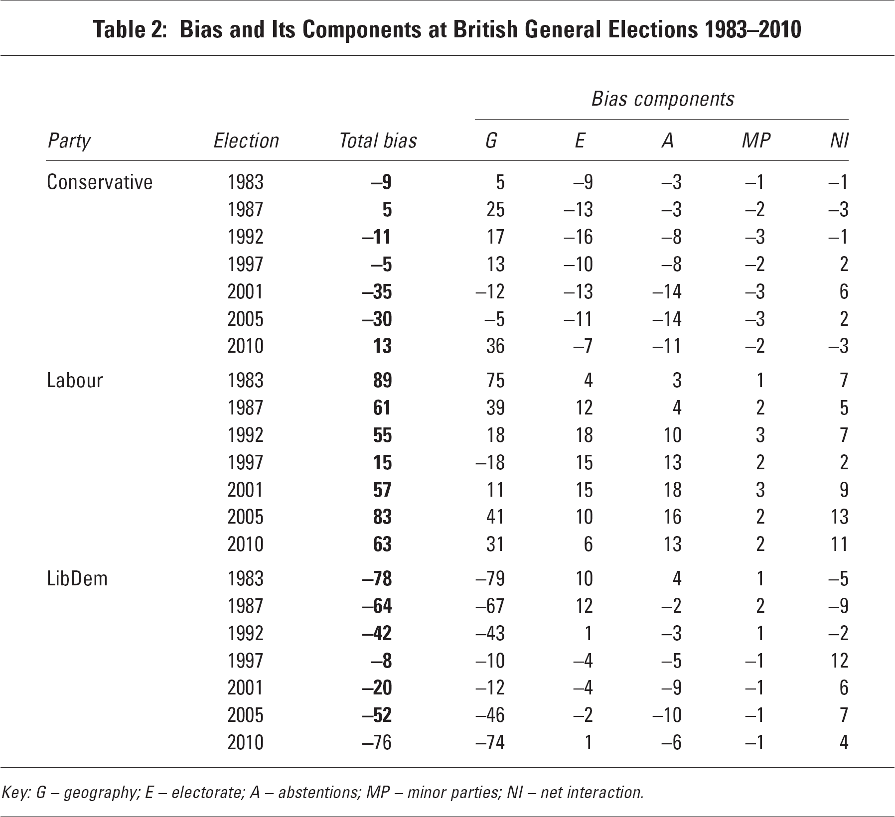
Key: G – geography; E – electorate; A – abstentions; MP – minor parties; NI – net interaction.
The second salient conclusion is that the Liberal Democrats suffered a net bias against them at all seven elections. Just as Labour's smallest advantage came in 1997, so did the Liberal Democrats' smallest disadvantage; it was the election where their vote and seat shares were closest (Table 1). The third salient aspect of this sequence of outcomes is that there was no consistent pattern in the treatment of the Conservatives: they experienced a positive net bias at two of the elections (which they won, including 2010) but were disadvantaged at the other five, substantially so in 2001 and 2005.
Table 2 identifies the size of the separate bias components which, like the net figures, can be interpreted as the number of seats' advantage or disadvantage that the parties experienced; a strong feature of Brookes' approach is its easily interpretable metric. Two features stand out with regard to the three ‘malapportionment’ components – electorate, abstentions and minor party: Labour has a positive advantage from all of them, whereas the Conservatives are disadvantaged in every case. In general, the Liberal Democrats are disadvantaged on all three, though they did benefit from winning relatively small constituencies in 1983 and 1987, when a substantial proportion of their victories occurred in Scotland and Wales, where constituencies have traditionally been much smaller than in England. 10
Of these three components, the impact of minor parties on the outcomes is, not surprisingly, small. 11 That of abstentions is quite substantial, however, with Labour the major beneficiary and the Conservatives the most disadvantaged. Turnout fell substantially over the period, reaching its nadir in 2001 at 59.1 per cent of the electorate. As it fell, Labour's advantage increased, because the percentage of abstainers tended to be larger in the seats that it won. 12
A similar difference characterises the Labour—Conservative comparison with regard to the electorate component: Labour benefited from its strength in the relatively small constituencies, whereas the Conservatives were disadvantaged by their relative strengths in the larger constituencies. Labour's advantage comes from three sources. The first is its relative strength vis-à-vis the Conservatives in the two parts of Great Britain with the smaller constituencies – Scotland and Wales – which was integral to the system. 13
Labour also benefits in respect of electorate size bias from variations within each country, especially England. This is partly a result of the Boundary Commissions producing constituencies with smaller electorates in Labour's heartlands (the inner cities and industrial areas). Because they have had to fit constituencies into the local government map and not cross county and borough boundaries unless the disparities between neighbouring constituencies are extreme, areas with small entitlements may get smaller seats than the average; most of those are in urban areas, where Labour tends to be the stronger party, notably but not only London, which has some of England's smallest constituencies (as well as some of its largest; counties tend not to have as many small seats). 14 In addition, Labour tends to benefit most from demographic changes subsequent to boundary revisions being accepted. The Commissions do not take projected population and electorate forecasts into account: they use the latest figures available at the start of their redistribution exercises to define constituencies with electorates ‘as equal as practicable’. As those constituencies ‘age’, some lose population and others grow – and areas of Labour strength tend to lose people. Thus, for example, in England the 1997, 2001 and 2005 elections were fought in constituencies originally defined on 1990 electorate data (i.e. they were some seven years out of date when first used). Of the 312 constituencies that Labour won at all three contests, the average electorate remained consistent at around 67,000, whereas in the 154 constituencies won by the Conservatives at all three it increased from 81,700 through 84,000 finally reaching 85,000 at the 2005 election.
These differences produced by the over-representation of Scotland and (especially after 2005) Wales relative to England, combined with the increasing variation in constituency electorates over time as they ‘age’, stimulated the Conservatives to propose the changes implemented in the Parliamentary Voting System and Constituencies Act 2011. These modified rules require every constituency with four exceptions to have electorates within +/−5 per cent of a UK-wide electoral quota (this is 76,641 for the first redistribution, which began in March 2011). 15 In addition, redistributions are to take place every five years so that each general election (under the Fixed Term Parliaments Act 2011) will be fought in a new set of equalised constituencies. In this way the Conservatives expect to remove the disadvantage that they have suffered from constituency size differences at every general election since 1959 (Johnston et al., 2001).
Why is Geography so Important?
The coalition government will probably remove (nearly?) all of one of the main sources of bias in the electoral system's current operation when new constituencies are defined under the 2011 Act, therefore. 16 But, as Table 2 shows, differences in electorate size are not a major contributor to the overall bias, never exceeding +/− eighteen seats for any one party. Indeed, at recent elections size differences have been less substantial than those associated with abstentions. Thus the changes introduced in the new legislation are unlikely to result in election outcomes that treat each of the parties equally – and certainly not the Liberal Democrats relative to the other two.
The impact of the geography of abstentions cannot be changed by legislation, other than by making voting compulsory; it reflects individual behaviour patterns. Hence there is no reason to explore it further here. But what of the geography component, which Table 2 shows was by far the largest in its impact on the translation of votes into seats at every election for the Liberal Democrats, and the largest for both Labour and the Conservatives at five of the seven elections? Furthermore, although this component was consistently a negative source of bias for the Liberal Democrats – a very large one at two of the elections – it was positive at some elections and negative at others for the remaining two parties, as well as varying very substantially in its size, especially for Labour (from +75 to −18).
The geography component, as already noted, reflects the efficiency – or effectiveness – of a party's distribution of votes across the constituencies, illustrated by dividing each party's achieved votes into three groups:
Surplus votes are those won in excess of the number needed to win in any constituency where it occupies first place; they are defined as the party's total number of votes obtained minus those won by the second-placed party, minus one. Thus if Labour wins 25,000 votes in constituency x and the Conservatives come second with 22,000, Labour has amassed 2,999 surplus votes. Wasted votes are those won in seats where a party loses (i.e. 22,000 Conservative votes are wasted in the above example). Effective votes are those needed for victory in seats that the party wins – as defined above (i.e. 22,001 of Labour's votes in that example).
Surplus and wasted votes do not contribute to winning seats, therefore; only effective votes do. It is thus in each party's interests to optimise its campaign efforts by maximising its effective votes and minimising the other two groups – which it can do by ‘winning small and losing big’: it should aim to win constituencies by only small majorities and in those seats where it is destined to lose it should accumulate few wasted votes and lose big. If a party was highly successful at that strategy, of course, it would be vulnerable to losing seats at the next election if there is a small swing against it, and would find it difficult to win other seats because of the large swing needed to overhaul the leading party locally. Nevertheless, at any one election, the closer its distribution of votes across the constituencies conforms to the maxim, ‘win small, lose big’, the better the outcome in the translation of votes into seats.
Table 3 gives the number of votes for each party and the percentage of these that were surplus, wasted and effective. The great majority of the Liberal Democrats' votes were wasted. They performed best in 2001 and 2005, when some 16 per cent of their votes were effective, but there was a fall-off in 2010: very few of their votes were surplus. This is the usual situation in an FPTP system when votes for a third-placed party are not spatially concentrated. 17 Few candidates win an election even in a three-party system with less than 40 per cent of the votes – in part because of the impact of small parties and independents even if the smallest of the three largest parties does not perform well (see Johnston and Pattie, 2011a). At the 2010 general election in England, for example, only 78 of the 532 seats contested by all three of the largest parties (i.e. excluding the Speaker's) were won with less than 40 per cent of the votes and just nine with less than 35 per cent. 18 Not only did the Liberal Democrats average well below that threshold at all of the elections being considered here, but they also had a relatively even distribution of their share across all constituencies: in 2010, for example, they had a mean constituency share of 23.1 per cent, with a standard deviation of 10.5, whereas for the Conservatives and Labour the comparable figures were 35.6 (standard deviation 14.6) and 31.0 (15.9), respectively. The geography of Liberal Democrat support resembles a plateau with few peaks or troughs, so while it continues to get between one-fifth and one-quarter of the votes it is unlikely to win many seats – or come close to victory in others.
Surplus, Wasted and Effective Vote Shares at British General Elections 1983–2010
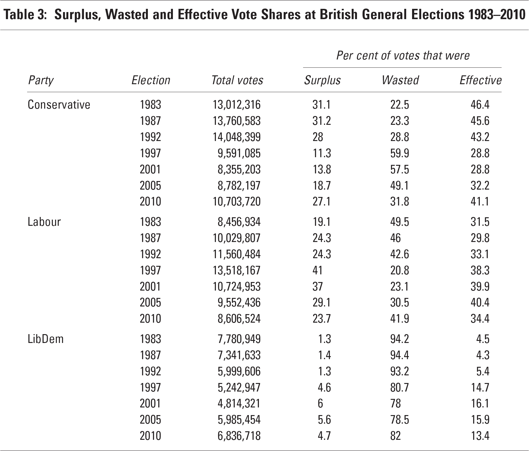
Turning to the other two parties, one clear difference is between the situations when they won and lost the election overall. Each had more than 40 per cent of its votes effective in the elections that it won, and less in those that it lost. The Conservatives had more effective votes when they won in 1983, 1987 and 1992 (averaging 45.1 per cent) than Labour at the subsequent three elections (an average of 39.5). The Conservatives also had a slightly higher percentage of effective votes in 2010 than did Labour with a similar share of the votes overall in 2005. At the three elections they lost, however, the Conservatives had a smaller percentage of effective votes (averaging 29.9 per cent) than did Labour at the four they lost (average 32.1).
One clear indicator of the efficiency of a party's vote distribution is its number of surplus votes. On this measure, the Conservatives clearly ‘outperform’ Labour: their average surplus percentage at their four victories was 29.3, compared with 35.7 for Labour at its three victories. Similarly, the Conservatives had many fewer surplus votes when they lost (an average of 14.6 per cent) than did Labour (average 22.8). Labour traditionally had a large number of very safe seats that it won by substantial majorities – mainly in mining and industrial areas where not only was its support base large but local trades unions mobilised substantial numbers of electors to vote. Although much of the industrial and union base to that support has been dissipated by post-1980 industrial change, nevertheless Labour still has these strongholds – a lot of them in Wales and Scotland – which deliver large percentages of surplus votes (even if the vote totals there are relatively small, because of both small electorate size and high abstention rates). This accounts for its large positive geography component at the 1983 and 1987 general elections (Table 2), and again in 2010. These were the elections when Labour performed particularly badly (getting around 30 per cent of the votes) and those relatively safe constituencies ensured that its seats share fell by less than was the case for the Conservatives in 1997–2005. When there was an overall swing of votes away from Labour this was not as exaggerated in the decline in the number of seats won as was the case when the Conservatives experienced a similar loss of support.
So why did Labour do so well in 1997 and 2001, when its seat share was more than 20 percentage points higher than its vote share? Its percentage of wasted votes was small – 20.8 and 23.1, respectively, probably because of tactical voting. During the campaign prior to the 1997 general election Labour and the Liberal Democrats were not only united in their desire to remove the Conservative government but also close on many policy issues, as both party leaders reported in their memoirs (Ashdown, 2009; Blair, 2010). Thus there was a great deal of (implicit and sometimes explicit, at least at the grass-roots level) encouragement to vote tactically where this could assist in the goal of defeating a Conservative candidate. Estimates suggest that substantial numbers did vote tactically (Johnston and Pattie, 2011b; Pattie and Johnston, 2010; Johnston et al., 2001, pp. 168–75) so where Labour was in third place its vote fell relatively, if not absolutely, thereby reducing its number of wasted votes: the second part at least of the ‘win small but lose big’ maxim certainly applied then. Tactical voting was again on the (implicit) agenda in 2001, to prevent a Conservative recovery, but there was something of a ‘tactical unwind’ in 2005 (Fisher and Curtice, 2006). It reappeared in 2010, however, as a result of further attempts by Labour and Liberal Democrat supporters to prevent a (large?) Conservative victory, although there were also some moves by Conservative and Liberal Democrat supporters to prevent a further Labour government ensuing (Johnston and Pattie, 2010; 2011b).
Skewed Distributions and the Conversion of Votes into Seats
Tactical voting illustrates how (party-induced in many cases) voter behaviour can influence the frequency distribution of a party's support across the constituencies. Figures 1–3 show the vote distributions for Conservative, Labour and Liberal Democrat parties for all seven elections since 1983. According to the ‘win small, lose big’ maxim, the most efficient distribution would be negatively skewed, and the least efficient positively skewed, with the mode in the region of 45–55 per cent. In a two-party system, a party with just over 50 per cent of the votes cast and a negatively skewed distribution would win a much larger share of the seats than of the votes, with the converse for a party having a positively skewed distribution (Gudgin and Taylor, 1979; Johnston et al., 2001). 19 In a three-party system in which one of them gets a substantially smaller share than the other two, a positive skew is desirable for that third party since with a relatively small share (<25 per cent) of the votes nationally a number of constituencies where its percentage is much greater than the average allows it to win some seats and establish a parliamentary presence. As it grows, however, it needs to change the shape of its distribution from a positive to a negative skew, which is a difficult task (although not impossible, as the post-war Labour experience demonstrates: it had an inefficient positive skew in the early decades, but a much more efficient negative skew by the 1990s–Johnston et al., 2002). The shape of the Liberal Democrat vote distribution has posed a considerable problem at recent elections: should the party invest limited campaigning resources in the relatively small number of seats where they have a chance of winning, thereby increasing their parliamentary cohort, or should they aim to broaden the geographical base of their support and build the foundations for shifting to a negatively skewed distribution (Denver, 2001)? Figure 3 indicates little change over the period: their geography of support was very positively skewed at all seven elections, a pattern quite different to Labour's (which is very platykurtic, with both positive and negative elements but with a long negative tail, especially in 1997 and 2001 when it benefited from tactical voting: Figure 2) and the Conservatives' (which is negatively skewed: Figure 1).
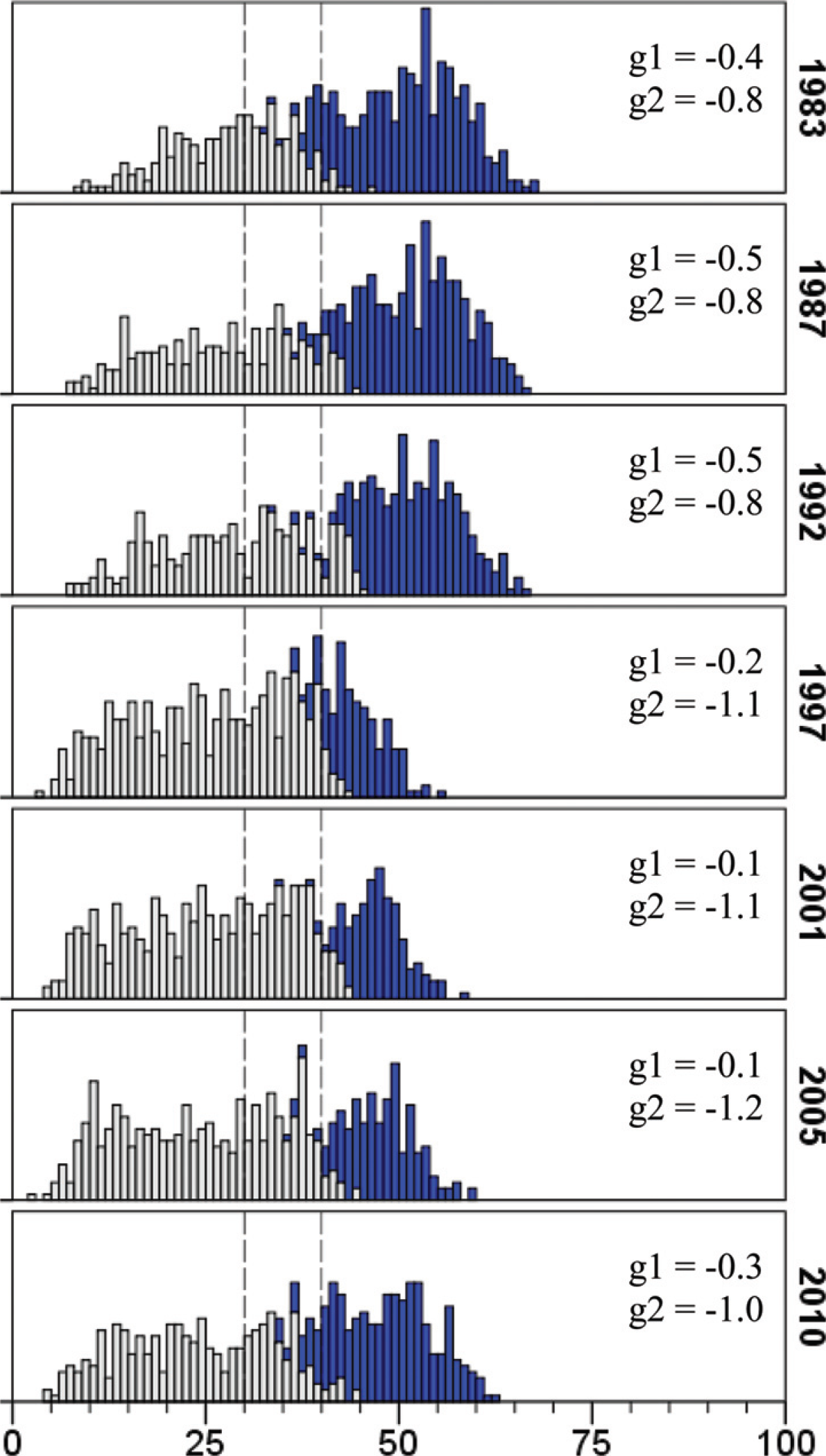
Conservative Share of Vote
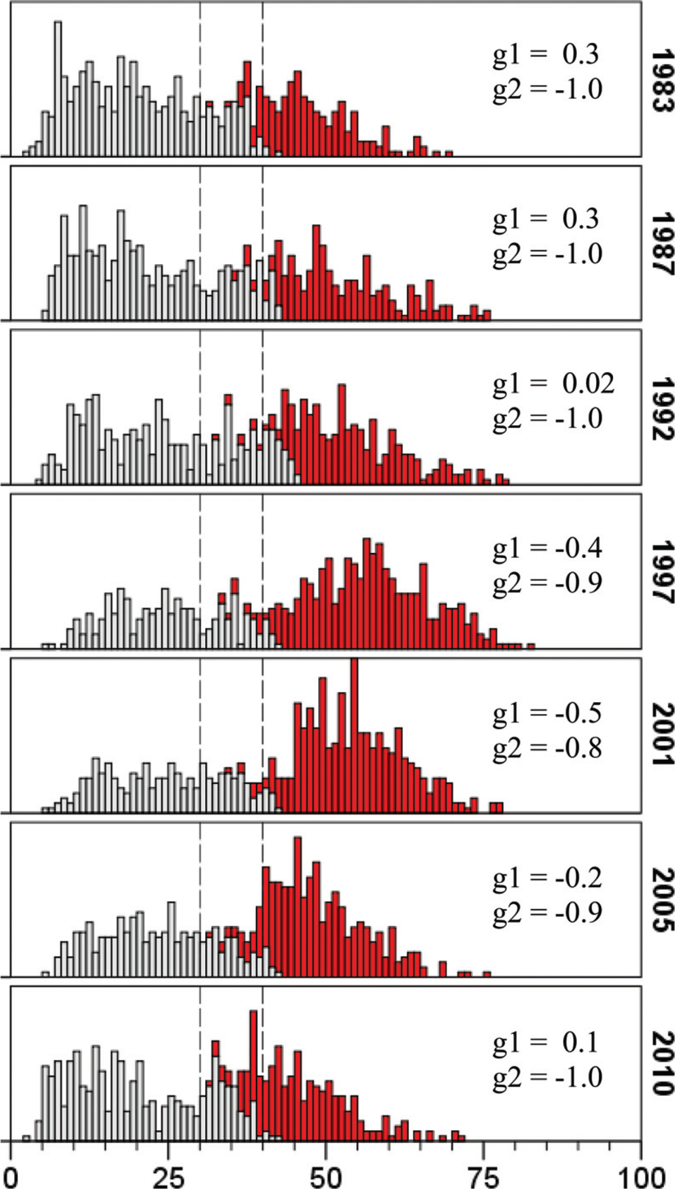
Labour Share of Vote
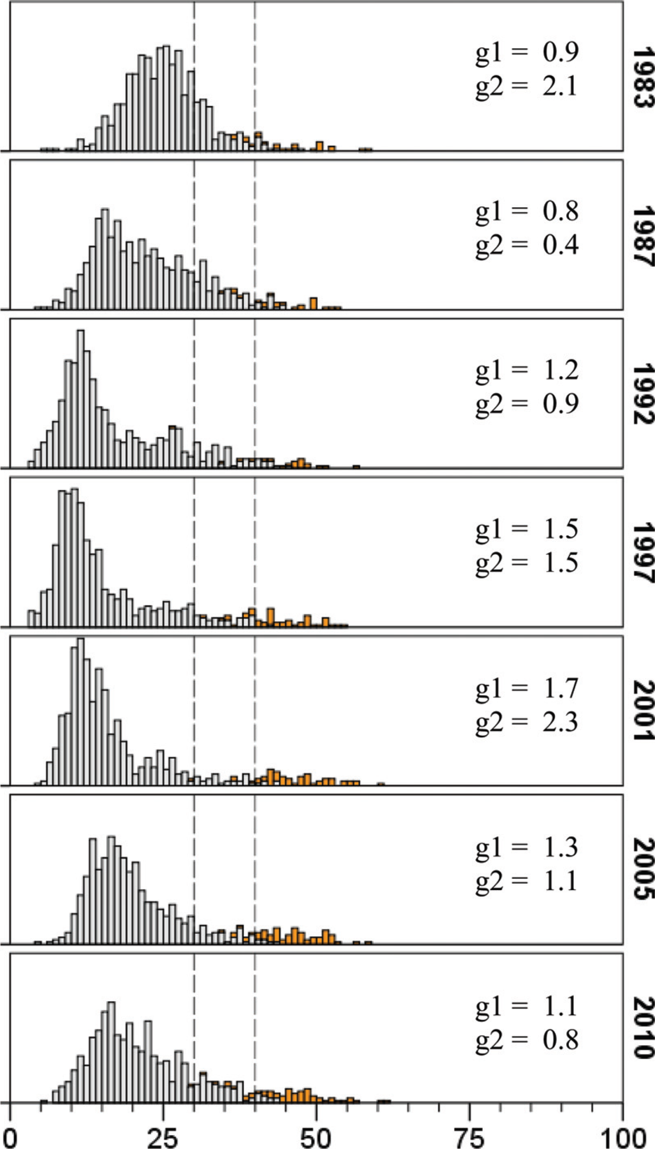
Liberal Democrat Share of Vote
In a two-party system, where minor parties gain only a very small share of the votes cast (as in Britain before the 1970s), the interconnection of the two parties' frequency distributions is crucial in determining the extent of the disproportionality and bias in general election outcomes. In a three-party system (or even a ‘two-and-a-half party system’, which is how some commentators describe the current British situation: Laakso, 1979; Siaroff, 2003) the interconnection of the three frequency distributions determines how their votes are translated into seats, a process further complicated by the impact of the smaller parties, which won 10 per cent of the votes cast in 2010. As the number of parties – large and small – increases, so the average percentage of the votes cast needed for victory is reduced in most constituencies. A share considerably below 40 per cent may deliver a constituency victory, especially if the three largest parties are all strong contenders. In 2010 only fifteen constituencies out of the 631 in Great Britain 20 had all three parties with 25 per cent or more of the votes – what might be identified as the ‘three-party marginals’. In a further 78 seats, however, all parties got 20 per cent or more – although in 26 of them the winning party had a margin of 20 or more percentage points over the second placed and in a further 22 the lead was between 10 and 20 points.
What is crucial for a party in such a situation, therefore, is whether it converts its share of the votes into winning the seat. Table 4 shows that in 2010 all three parties won all of the seats where they obtained 45 per cent or more of the votes cast, and there was only one case where a party won with less than 30 per cent (the Liberal Democrats in Norwich South). 21 Crucial, therefore, is relative success in converting votes into seats where a party's share falls between 30 and 45 per cent. In 2010 there were very considerable differences among the parties in this respect. Labour won virtually all of the seats where it gained between 40 and 45 per cent of the votes, for example, whereas the Conservatives failed to win eleven of the 77 where it was in that position, and the Liberal Democrats failed to win as many as half. It was the same where the parties gained 30–40 per cent of the total; Labour achieved victory in 38 per cent compared to 26 per cent for the Conservatives and only 11 per cent for the Liberal Democrats.
From Votes to Seats at the 2010 British General Election
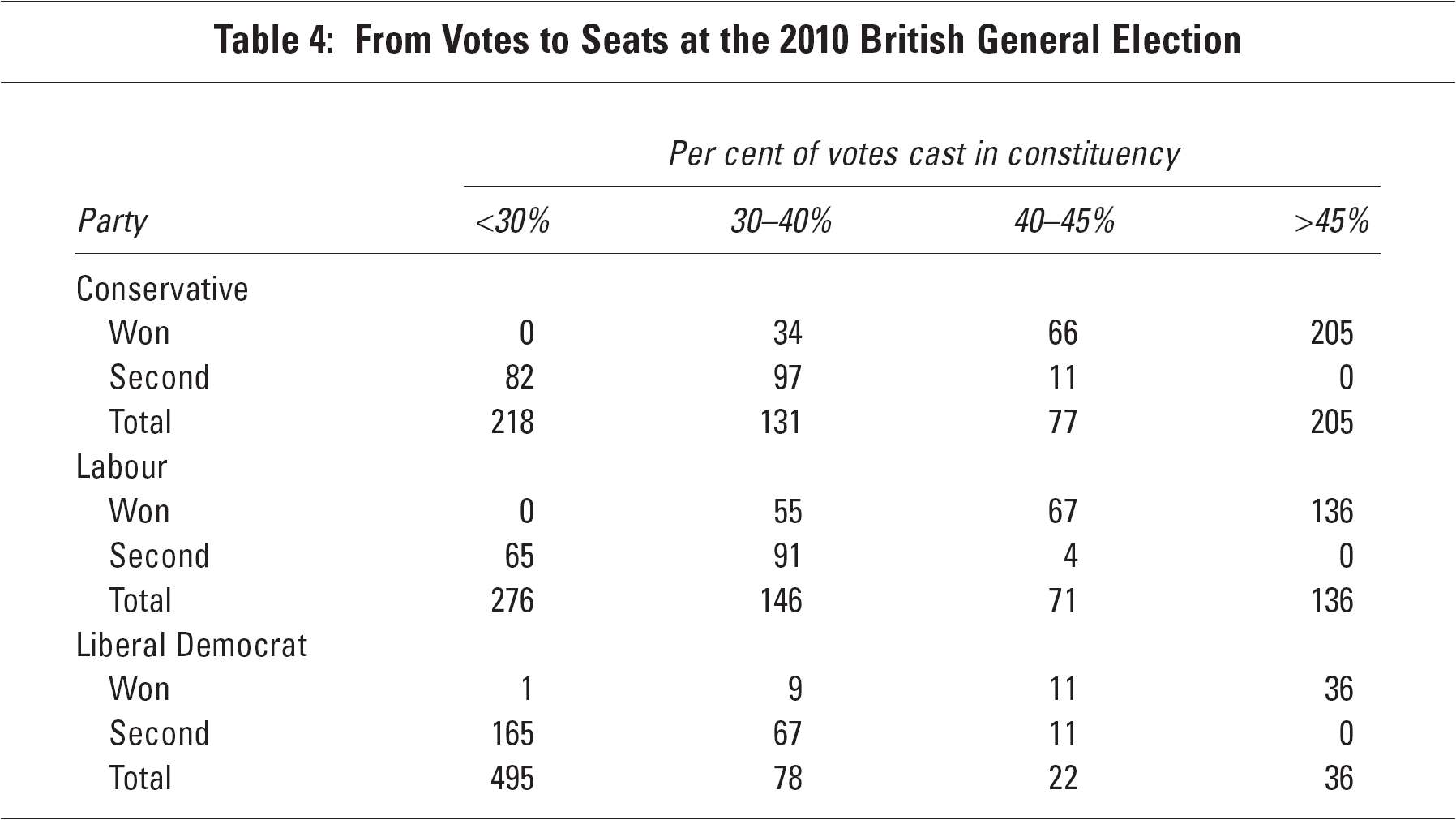
Why this difference? One possibility is that Labour was more likely to get 30–45 per cent of the votes in Scottish and Welsh constituencies where the presence of a fourth substantial party nationally (the SNP and PC, respectively) meant that on average a smaller share of the votes cast was likely to result in a constituency victory than was the case in England, where in most constituencies there was no comparable fourth party. (Apart from the three incumbent independent MPs, all of whom lost their seats, there were only eight English constituencies where at least one of the small party candidates won 10 per cent or more of the votes). 22 Indeed, of the 112 seats where Labour won with 30–45 per cent of the votes, 28 were in Scotland or Wales (where it lost just 8 seats with that share of the votes); for the Conservatives, only 8 of their victories in that vote share band were in Scotland or Wales (where they also lost 14); 23 and the Liberal Democrats won 9 of the 18 seats there where they won 30–45 per cent of the votes. 24
Apart from this difference between the three parties in their relative strengths in England, Scotland and Wales, a further difference in their ability to convert a vote share of 30–45 per cent into a constituency victory reflects their geographies of support. In effect, Labour was better able to win in the constituencies where the three main parties were relatively equal – that is, those that came closest to being three-way marginals. This can be illustrated by computing a simple statistic PCS:

where shLabi, shConi and shLDi are the Labour, Conservative and Liberal Democrat percentages of the total number of votes cast for those three parties only in constituency i. This statistic shows how far away each constituency is from the ‘equal shares’ situation (perfect three-party competition). The smaller the value of PCSi, the more three-way marginal is the seat. In England, constituencies where Labour obtained between 30 and 45 per cent of the three-party votes had an average PCS of 18 whereas the mean PCS values in similar Conservative or Liberal Democrat seats were 21 and 25, respectively. On average, therefore, seats where Labour got 30–45 per cent of the votes in 2010 were also more likely to be three-way marginals than was the case with the other two parties, hence its higher conversion rate. 25
As the three frequency distributions shown in Figures 1–3 move between elections, as each party's constituency average share of the votes changes and, to the extent that the changes in individual constituencies vary from a uniform swing, the distributions also change shape, so the conversion rates should alter. Table 5 shows in more detail those rates for two percentage share bands – 30–40 and 30–45 – at the seven general elections from 1983 on, plus the narrower 40–45 percentage share band; most parties would expect to win a constituency with that share in a three-party contest. A number of main conclusions stand out.
Conversion Rates: Percentage of Seats Won by Each Party with Different Shares of the Vote Total
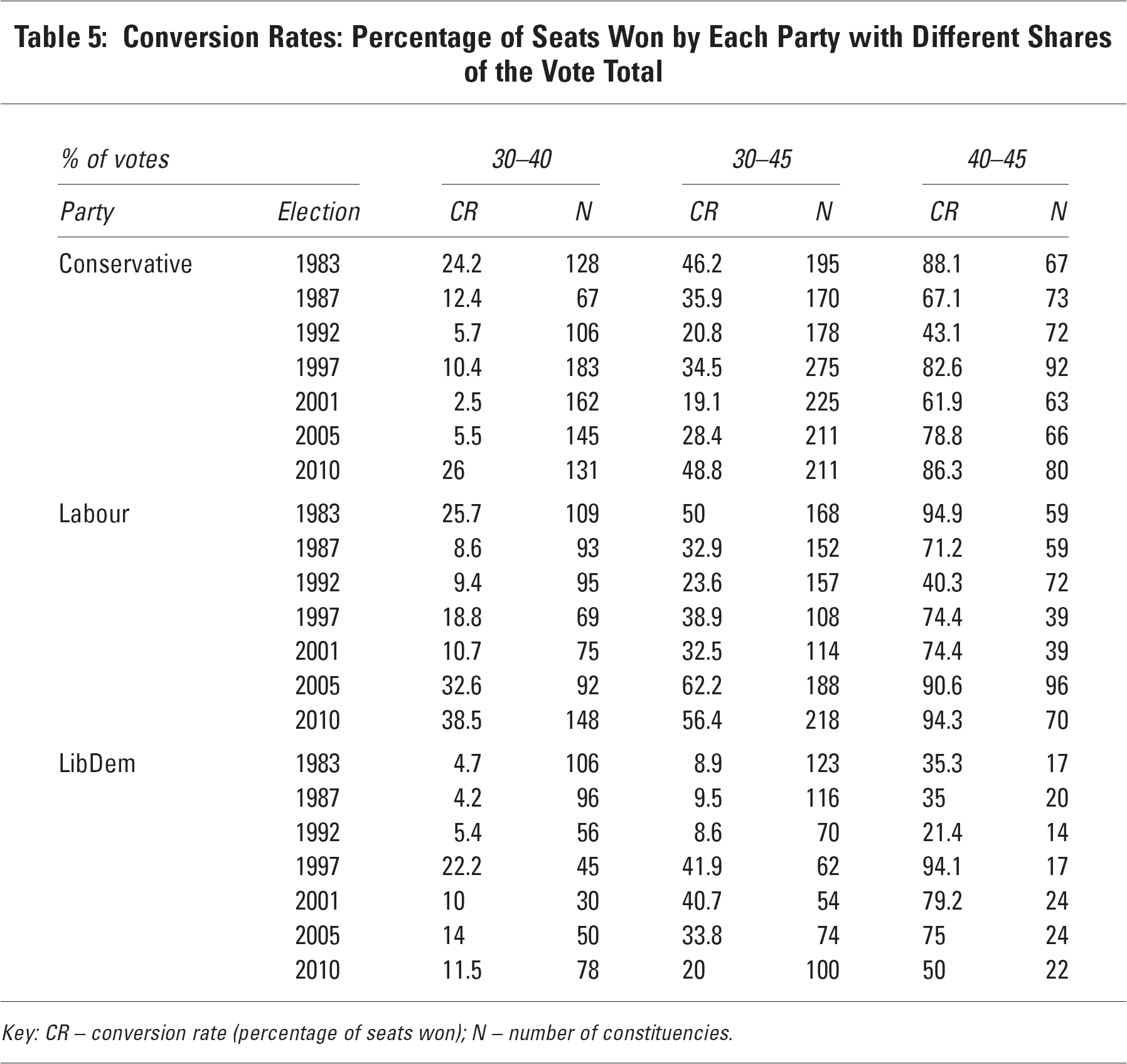
Key: CR – conversion rate (percentage of seats won); N – number of constituencies.
At the first three elections the conversion rates for the Liberal Democrats were much smaller than those for the other two parties in all three bands. Whatever their vote share between 30 and 45 per cent, the Liberal Democrats were less likely to win the seats than either Labour or the Conservatives, in some cases by a very large margin: in 1983, for example, the Conservatives won 88 per cent of the 67 seats where they got 40–45 per cent, and Labour won 95 per cent of the 59 seats with that share, but the Liberal Democrats' conversion rate was only 35 per cent of the 17 seats. That party's best performance was in 1997, when it won 22 per cent of the seats where it gained 30–40 per cent, 42 per cent where its share was between 30 and 45, and 94 per cent where it was 40–45. But it declined thereafter.
For the other two parties, the clearest difference is for the 2001–10 elections when Labour had substantially larger conversion rates in each band than the Conservatives; in 2005 Labour won 62.2 per cent of the seats where it gained 30–45 per cent of the votes, and 90.6 per cent of those where its share was 40–45, compared to figures of 28.4 and 78.8 per cent, respectively, for the Conservatives. Prior to that, however, the differences between the two were slight and largely patternless – although both had very low conversion rates, even in the 40–45 per cent vote share band, at the 1992 election.
The importance of the geography component to the overall bias in recent UK general election results – how efficiently each of the parties' votes are distributed across the constituencies – is thus a function of two separate factors. The first is the frequency distribution of each party's vote shares: the degree and direction of skewness is a crucial determinant of the efficiency of the process whereby votes are translated into seats. But the nature of the skewed distributions cannot account for all of the inter-party variation in the ratios of seats to votes because of variations in the percentages of their votes that were either surplus, wasted or effective (Table 3). The relative proportions of each party's votes in those three categories is apparently largely a function of variations in their success rates at winning seats when their vote share falls in the range 30–45 per cent. Below the lower figure, each party almost invariably failed to win the constituency whereas above that figure victory was assured (Table 4).
Crucial to appreciating the variations in conversion rates within that vote range is the nature of the local competitive situation. The likelihood of a party winning a seat if its vote share lies between 30 and 45 per cent depends on its competitors' relative performance. If, for example, Labour had between 30 and 45 per cent of a constituency's votes and both the Conservatives and the Liberal Democrats had a substantial share of the total too, then Labour's chances of success increased – three-way marginals are necessarily won with smaller vote shares. In addition, the better the aggregated performance of the minor/other parties, the smaller the vote share that one of the three large parties needs for victory. In a close three-way marginal constituency where the minor parties win 10 per cent of the votes, victory is quite likely for one of the major parties with just 33 per cent; where the minor parties get only 2 per cent between them, 36 per cent may be needed. On the other hand, in a constituency where the third party gets only about 15 per cent of the votes, and where the minor parties win 10 per cent, then a share of around 38 per cent is probably needed by one of the other two. 26
Conclusions
In the context of contemporary electoral reform debates, the analyses presented here have more than sustained the Liberal Democrats' opposition to the first-past-the-post system. The Conservatives have also been disadvantaged at most of the recent elections. Their analyses of that situation have focused on differences in constituency electorates and the legislation passed in 2011 is designed to correct that. But the disadvantage they have suffered from the electorate size component has been small – as has Labour's advantage – and although removing its cause would eliminate that bias element, which could be crucial in a close contest, it does not mean a ‘level playing field’ in future contests between them and Labour (Thrasher et al., 2011).
The geography of a party's votes – how efficiently they are distributed across the constituencies – is crucial to the creation of biased election results in the UK. Part of the reason – as others have shown (e.g. Gudgin and Taylor, 1979; Johnston et al., 2002) – lies in the frequency distribution of each party's vote shares: certain distributions – where the party ‘wins small but loses big’– produce better outcomes than others. Vote distribution profiles for the three main parties since 1983 reflect patterns of voter behaviour (and of party behaviour in their efforts to mobilise support, which is spatially very variable: Denver and Hands, 1997; Pattie and Johnston, 2009) which are not readily manipulated. Studies of campaign effects show that the more intensive a party's campaign in a constituency the better, ceteris paribus, its performance there (Johnston and Pattie, 2008), so the geography of party activity and resources is crucial. 27 That is open to manipulation at the margin through the encouragement of tactical voting – and, at the extreme, by parties agreeing not to field candidates against each other in particular circumstances, which occurred with the Alliance of the Liberals and Social Democrats in 1983 and 1987.
But as our analyses of conversion rates have shown, the interrelationships of those distributions is also crucial. Where the contest between all three of the largest parties is relatively close, then a seat may be won with less than 35 per cent of the votes – especially if one or more of the minor parties also performs well. Conversely, a party may capture above 40 per cent of the constituency vote and still lose to a stronger rival.
In a country where two parties predominate and there is not only either malapportionment or gerrymandering but also the parameters of the first-past-the-post electoral system (how constituencies are defined) and the geographies of party support show no peculiarities, then election results are largely predictable. But as the situation moves towards a three-party system, with smaller parties also winning more than a trivial share of the votes, the election outcomes become less predictable and more likely to be biased. This is the current British situation and its appreciation calls for a method that can unravel the causes of bias. That has been achieved here, using a modification of a well-tried measure of bias in two-party systems to take account of the three-party situation.
Unpredictability is a marked feature of recent British election results, which raises questions about the electoral system's ‘fitness for purpose’ (Curtice, 2009; 2010). So much depends on the interrelationships between a series of geographies; we can successfully predict what will happen when they interact in particular ways – but not when those situations will emerge. The minimal electoral reform undertaken by the Conservatives substantially to reduce variations in constituency size will not change that situation markedly.
Footnotes
3
In the negotiations over the possibility of a Labour—Liberal Democrat coalition being formed immediately after the 2010 election, it is suggested that Labour offered to make the change to AV without a referendum although ![]() , pp. 548–9) suggests that holding a referendum in autumn 2010 remained the plan.
, pp. 548–9) suggests that holding a referendum in autumn 2010 remained the plan.
5
6
For the full sequence of bias estimates calculated in that way for the seven elections since 1983 see Borisyuk et al. (2010); Johnston et al. (2001); ![]() . In addition to this ‘equal shares’ approach Brookes also allowed for a procedure that involved reversing the shares of the two main parties which gave similar, though not identical, bias estimates.
. In addition to this ‘equal shares’ approach Brookes also allowed for a procedure that involved reversing the shares of the two main parties which gave similar, though not identical, bias estimates.
7
Blau (2001; ![]() ) has presented a reasoned critique of this approach and proposed an alternative method, which reaches very similar conclusions about the size, direction and components of the observed bias.
) has presented a reasoned critique of this approach and proposed an alternative method, which reaches very similar conclusions about the size, direction and components of the observed bias.
8
The interaction term may also encompass some ‘random noise’– bias towards or against the particular party that is not identified with one of the main components.
9
Although we use the term ‘beneficiary’ or ‘advantage’ elsewhere there is no suggestion that a party is deliberately engineering this situation but rather that it so happens that a given electoral situation is better for it than its rivals. The method of measuring electoral bias is simply one way of offering a detailed description of parties' electoral gains and losses.
10
The average constituency in England in 1987 had 68,806 electors; for Scotland and Wales the averages were 54,895 and 56,614, respectively. The constituencies won by the Liberals in Wales averaged 51,474 electors; those won in Scotland averaged 51,154. From 2000 on, Scottish constituencies had to be defined using the same electoral quota as England, but they were still smaller on average than those in England at the 2010 election (65,500 in Scotland and 71,680 in England) because of the small constituencies in the Scottish Highlands and Islands where ‘special geographical considerations’ were invoked by the Boundary Commission during its 2004 redistribution. The average Welsh constituency had 56,500 electors in 2010.
11
The SNP and Plaid Cymru contested only a minority of the constituencies and – with the exception of the Greens in 2010 and a small number of independents at the earlier elections – no other parties came close to victory in any constituency.
12
The average turnout in Labour-won seats in 2001 was 56.7 per cent, compared to 63.0 per cent in those won by the Conservatives and 63.8 per cent in those won by the Liberal Democrats.
13
Wales was guaranteed at least 35 seats in the 1944 House of Commons (Redistribution of Seats) Act and Scotland 71; the figure for Great Britain should be not substantially greater or less than 613, leaving 507 for England. Over time, the number has grown, more rapidly in England than in the other two countries but not sufficiently so as to counter differentials in their rates of population growth. By 2001, Wales had 40 seats, Scotland 72 and England 629. Scotland's number was reduced to 59 in 2005 as part of the 1998 devolution settlement (see above, Note 10) but Wales' complement remained unchanged at 40, and England's was increased before the 2010 election to 533. Because Labour is relatively stronger in Wales and Scotland than in England – it won 34 of the 40 Welsh seats in 2001 (85 per cent) and 56 of Scotland's 72 (78 per cent), as against 323 of England's 529 (61 per cent) – it benefits from their smaller constituencies in the votes-to-seats translation, as reflected in that bias component.
14
For example, if the electoral quota were 72,000, a borough with 194,400 electors would be entitled to 2.7 constituencies: it would be allocated 3, with an average electorate of 64,800; a county with an electorate of 914,400 would be entitled to 12.7; it would be allocated 13, averaging 70,340 electors. On the other hand, a borough with 165,600 electors would be allocated 2 (against an entitlement of 2.3) averaging 82,800 each, whereas one with 885,600 (entitlement 12.3) would have 12 constituencies averaging 73,800. The smaller the local government unit the larger the average deviation of constituency electorates from the quota – and most of the areas with small constituencies tend to be in cities where Labour is the stronger of the two main parties.
15
16
The exceptions to the +/−5 per cent rule are the Scottish constituencies of Orkney & Shetland (33,085 electors at the 2010 general election), H-Eileanan An Iar (the Western Isles – 22,266) and the Isle of Wight (which had one seat for 109,966 electors in 2010, but has been allocated two under the Act).
17
This is the case, for example, with the Bloc Québécois in Canada, which gets a share of the seats commensurate with vote share because votes are all concentrated in one province (LeDuc, 2007). In the UK, Plaid Cymru's votes are significantly concentrated within Wales, so that with 0.56 per cent of the UK total it obtained a reasonably proportional share of the 650 seats with three (0.46 per cent); the SNP was less successful, however, as with 1.65 per cent of the votes it obtained only 6 seats (0.92 per cent).
18
One was won with only 29.4 per cent: by the Liberal Democrats in a three-way marginal contest (Norwich South), where Labour won 28.7 per cent and the Conservatives 23.0. The Green party candidate won 14.9 per cent and three others shared the remaining 4.1 percentage points.
19
This was the basis for some of the early attempts to measure ‘electoral bias/distorted representation’ (Gudgin and Taylor, 1979; Johnston, 1979).
20
The number of seats is one less than the full total of 632 because, in line with established practice, the incumbent Speaker was not challenged by the main parties.
21
This was a rare ‘three-and-a-half-way marginal’: the Liberal Democrats won 29.4 per cent, Labour 28.7 per cent, the Conservatives 22.9 per cent and the Greens 14.9.
22
The BNP did so in Barking, Dagenham & Rainham, and Rotherham; the Greens did in Brighton Pavilion (which they won) and Norwich South; and Respect did in Bethnal Green & Bow, Birmingham Hall Green and Poplar & Limehouse.
23
In all eight of the Conservative victories only two parties got over 20 per cent of the votes and in none of these did either the SNP or PC get over 20 per cent. The Conservatives' successes in those two countries were all in ‘straight fights’ with Labour.
24
Parts of rural Scotland and Wales have long been Liberal heartlands.
25
A similar sequence of values (55.7, 57.3 and 59.8) emerges if the percentage shares used in the formula apply to all parties contesting the seat rather than just the ‘big three’.
26
Detailed analyses using Mann-Whitney U-tests, not reported here, show that each party was significantly more likely to win a seat with a vote share in the 30–45 per cent range if either (a) the third-placed party performed well or/and (b) the minor parties performed well.
27
As exemplified by the Conservatives' successful target seats strategy in 2010 (Ashcroft, 2010; Johnston and Pattie, 2010).