
Abstract
This article examines the relationship between economic inequality, electoral turnout and redistributive spending. I use the Current Population Survey to create direct measures of the income of the median voter to investigate its effect on spending and its relationship with inequality and turnout. In the 50 US states from 1978 to 2002, I find little effect of these direct measures on redistributive outcomes; nor do the individual characteristics of the median voter appear to mediate the effects of turnout and inequality measured at the state level. Thus I find no support for the contention that turnout affects government spending via increasing the political representation of the poor. In contrast to cross-national findings, across US states the income of the median voter is not strongly affected by turnout, but rather by other state characteristics.
What effect do economic inequality and political participation have on government spending? Greater representation of the poor, usually associated with higher turnout, is thought to increase government spending. Increased inequality increases the incentives for the less well off to demand redistribution from the rich. Both of these expectations are premised on the idea that individual preferences, dictated by economic situation, are translated into policy via participation in the political process. The logic is straightforward: the poorer the decisive voter, the more likely he or she will demand redistributive policies from government. The income of the decisive voter depends on two parameters: the distribution of income, and who votes. Much empirical work has studied the effects of these two variables – income inequality and turnout – on redistribution, or on government spending. Yet they are thought to be important only in that they impact the income of the median voter. In this article, I use direct measures, from individual survey data, of the income of the median voter and examine its effect on government spending.
Using data from the Current Population Survey (CPS) (US Census Bureau, 2006) for the US states from 1978 to 2002, I find that neither the income of the median voter, nor the shortfall between median voter income and mean income levels, materially affect the level of welfare spending as predicted by the model. Further, the effects of turnout and inequality, measured at the state level, as has been typical in previous work, retain what effects they have on spending when modelled simultaneously with the direct measures of median voter income. This suggests that they may be operating via a mechanism distinct from any effect on individual preferences; and there is also some evidence that they do not determine the identity of the median voter in income terms in as straightforward a fashion as is often assumed. I thus examine other factors that may affect the median voter's income level once turnout falls from universal levels.
Conventional wisdom holds that, given an income bias in voting, increased participation will increase the representation of the poor, and thus lead to greater government spending. This is consistent with a logic whereby the more people who vote, the lower down the income distribution is the pivotal voter. The Downsian logic of majoritarian democracies implies that it is the median voter who will be pivotal (Downs, 1957). Increased inequality gives the median voter more incentive to vote for redistributive policies since, other things being equal, the gains from redistribution are increasing in the difference between mean and median income (Meltzer and Richard, 1981). Conversely, an increase in turnout (assuming the increase is concentrated at the lower end of the income distribution) effectively moves the median down the income ranking, again increasing the political demand for redistribution.
The existing empirical literature finds (to generalise; see the discussion below) fairly consistent effects of turnout on government spending, and more mixed results for the effect of inequality and its interaction with turnout. This empirical analysis is the main focus here, and the major contribution of this article is to go beyond using turnout and inequality data – assumed to be important due to their impact on the income of the median voter – as proxies, and use the relevant data on the median voter's income directly. The results indicate that a re-conceptualisation of the mechanism by which turnout affects the income of the median voter is in order, and I note some possibilities for macro-level explanations. In terms of inequality, this article continues in the tradition of failing to find support for the implications of the Meltzer-Richard model.
Turnout and Redistributive Policy
The level of electoral turnout, as well as a class bias in the population of voters, has been found to affect government redistribution both in analyses of American states and in comparisons of developed countries. Much of the literature on the effects of turnout has come from the United States, where the focus has been on whether higher turnout would benefit the Democrats (Citrin et al., 2003; De Nardo, 1980; Nagel and McNulty, 1996) but there is little evidence here that Democratic candidates are disadvantaged by lower turnout. However, there could be effects on policy even without partisan advantage if both parties tailored their platforms in anticipation of a pro-rich bias in voting. Indeed, redistributive public policies are more generous where the poor are better represented (Hill and Leighley, 1992). A parallel comparative literature has also considered whether leftist parties do better as turnout rates increase (Pacek and Radcliffe, 1995), and does find a positive effect. Alexander Hicks and Duane Swank (1992) find that in addition to government partisanship, turnout increases welfare spending in the advanced democracies. Taking a broader view, the increase in ‘turnout’ associated with the extension of the franchise or transition to democracy leads to a transformation of the role of the state in the economy along more redistributive lines (Boix, 2003), although this conclusion has its critics (Ansell and Samuels, 2010). Most recently, Vincent Mahler (2006; 2008) investigates not only the effect of turnout on redistribution, but also the effect of turnout on the income skew in the electorate. This work finds that across countries turnout is positively related to redistribution. Further, this is due to the different skew induced in the income distribution of voters by different levels of turnout.
These macro-level findings fit well with the empirical literature on the characteristics of voters as compared to non-voters. Those who vote tend to be richer and better educated than those who do not vote (Verba et al., 1993; Wolfinger and Rosenstone, 1980). In addition, although the evidence that voters have different policy preferences from non-voters is mixed (Gant and Lyons, 1993; Wolfinger and Rosenstone, 1980), the most consistent differences are found with respect to redistributive policies (Bennett and Resnick, 1990).
Inequality and Redistributive Policy
If voter income determines preferences and the choice of policy, then inequality of income will have an impact on redistributive policy. Intuitively, since political resources in a democracy are distributed equally, the poor can use their relative numerical advantage to equalise the distribution of income. The greater the concentration of wealth, the greater the incentive to redistribute. This logic is formalised in the Meltzer-Richard model of redistribution (Meltzer and Richard, 1981). The key parameter is the difference between the income of the median compared to that of the mean, because the median voter is the ‘pivotal’ political agent (in a majoritarian democracy), while the mean income is the individual who exactly breaks even in a system of lump sum redistribution financed from linear taxation.
Empirical studies of the effect of inequality on redistribution, however, have found at best mixed support for the Meltzer-Richard model. Roberto Perotti (1996) looks at several different measures of redistribution across countries in an investigation of the mechanisms by which inequality could affect growth, but finds little consistent relationship between inequality and redistribution. Francisco Rodriguiez (1999) tries to test the Meltzer-Richard theory directly using both time series and cross-sectional (across states) data from the United States and finds neither a short-term nor a long-term effect of inequality on redistributive spending. Other studies have revealed negative relationships between inequality and redistribution (Lindert, 2004; Moene and Wallerstein, 2001), although this finding tends to be fragile across different model specifications (Iversen, 2005). Recent analyses focused directly on redistribution, rather than government spending measures, have tended to find the predicted, positive, association between inequality and redistribution (Kenworthy and Pontusson, 2005; Mahler, 2006; 2008; Milanovic, 2000).
Many, though not all, of these analyses include the level of turnout as a control variable. However, if the median voter mechanism is to be taken seriously, the interaction of turnout and inequality is a critical variable, which has been little studied. Robert Franzese finds that the interaction does have the predicted effect on redistribution in the advanced democracies he studies (Franzese, 1998; 2002); yet other work explicitly considering this interaction term finds no effect (Ansell and Samuels, 2010; Boix, 2003). A further refinement, bringing the empirical analysis closer to the model, investigates not only the effect of turnout but also the skew that inequality in turnout induces in the income distribution of voters. Using macro-level data, Henning Finseraas (2008) finds no evidence that the effect of inequality on redistribution is contingent on voter turnout, and explains this with survey data revealing that low turnout in fact advantages parties of the left.
These models are all based on a model of the relationship between turnout, inequality and redistribution that is grounded in the micro-logic of the median voter. The accounts of the effects of turnout follow a similar underlying logic where the outcomes of the policy-making process depend on the representation of individual preferences in the political system, even if they are less explicit about whose preferences matter. The same logic underpins the accounts as to why each of these independent variables affects redistribution (Larcinese, 2007). It is worthwhile making this model explicit, to reveal best the implications that can be taken to the data.
In the workhorse Meltzer-Richard model linking inequality to redistributive preferences, everybody votes on a linear tax rate to finance lump sum redistribution. Thus the individual with average (mean) income by definition ‘breaks even’ through the tax and benefit system. Assuming some elasticity in labour supply, Meltzer and Richard derive the result that an individual's preferred tax rate is inversely ordered by income. The further an individual's income below the mean, in dollar terms, the higher tax rate they will choose. Thus individuals will demand redistribution in proportion to the extent by which mean income exceeds their own income. It is this particular kind of inequality that should be associated with rising redistributive demands.
More broadly, the same intuition applies: more inequality implies a concentration of resources at the high end of the distribution, providing more resources for redistribution from the perspective of individuals – voters – with incomes below the average. Stepping outside the strict median voter framework the same logic also implies that the greater the concentration of resources at the top, the more individuals there will be whose incomes lie below the mean and who will thus favour redistributive policies.
Turnout and the Median Voter
The translation of these preferences into policy relies upon the median voter as the decisive voter in a majoritarian system. When the median voter is pivotal, the relevant metric for inequality is the difference between median and mean income. Non-participation at the bottom of the income distribution moves the median voter's income up, relative to the median income in the population. On a Meltzer-Richard logic this translates directly into lower redistribution. Assuming that the income distribution remains the same, the median voter's income is determined by the distribution of voting in the population. The maintained assumption in the literature linking turnout to policy outcomes is that as turnout declines, abstention is concentrated among low-income voters. Thus higher turnout leads to lower median voter income. This translates into a bigger gap between median voter income and the average income in the population.
In many analyses of the effect of turnout on redistributive policies, this median voter mechanism is not explicitly cited as the way in which the preferences that are represented in the political process are determined. The notion that no heed need be taken of those who do not participate, however, is clear (Lijphart, 1997). Also, while there are many other ways to influence policy beyond voting (Schlozman et al., 2008), the effect of turnout itself requires a logic of the representation of individual preferences.
Thus we are left with a model at the macro level whereby redistributive policies are essentially a function of the income of the pivotal voter, relative to mean income. This parameter is determined by two things: the distribution of income, and who votes. The theoretical models either implicit or explicit in the literature outline a logic of individual preferences which therefore imply that:
the income of the median voter (relative to average income) affects the level of redistribution; the effect of turnout on redistribution runs through its effect on the income level of the median voter; the effect of income inequality on redistribution runs through its effect on the income of the median voter.
It is these latter two hypotheses that analyses of the interaction of turnout and inequality are essentially testing. In this article, however, I am able to test directly the step in the logic that is implied by the interaction model, namely that the income of the pivotal voter determines redistributive policies.
Empirical Analysis
I proceed with three empirical strategies to investigate the influence of the income of the pivotal voter on redistributive policy, and the implications for turnout and inequality. First, I estimate the effect of the shortfall of the median voter's income, relative to the mean, on redistribution. Second, I consider whether the effect of turnout on redistribution is mediated by the income of the median voter, as it should be if the individual-level, median voter logic applies as is implied by the model, and also the obverse case, whether the impact of inequality is mediated by turnout. The results give only limited support for the intuition behind the conventional wisdom. To make sense of these two sets of results, therefore, I explore the effect of macro-measures typical in the literature on the income of the pivotal voter.
Data and Methodology
The analysis that follows is a time series cross-section of the 50 US states (excluding the District of Columbia) from 1978 to 2002. While much of the literature on inequality and redistribution uses cross-national comparison, comparing sub-national units has the advantage of greater similarity of both institutional and cultural characteristics. The drawback of comparing states as opposed to nations is the potential for a lack of variation on the dependent variable. However, the individual US states are responsible for two of the most important programmes of redistribution, Supplemental Security Income (SSI) and ‘welfare’: Aid to Families with Dependent Children (AFDC) and Temporary Aid to Needy Families (TANF) after 1996. These programmes constitute a significant proportion of the redistributive effort made in the United States, and there is considerable variation in the generosity of benefits across states. In 2004 the average monthly TANF payment to a family with three children was $420, but levels ranged from $170 to $923 (Lazere and Tallent, 2006). There is also a large degree of variation in total state expenditure. Since this captures all the services provided by the state, to the extent that these are ‘lump sum’ benefits paid for through proportional taxation, this is a better measure of the ‘redistribution’ that the Meltzer-Richard model seeks to explain.
One complication in considering the sub-national data is that budget decisions at that level are taken in the context of the federal system. While many state constitutions do require balanced budgets eliminating the scope for borrowing to fund expenditures (as assumed by the Meltzer-Richard model), the taxes that fund redistribution within a state need not come from within that state, as a substantial share of state revenues comes from federal grants. The link between state taxation and state spending is thus weakened by federal expenditures. Furthermore, this effect varies across states, as some states contribute more in taxation than they receive in federal grants, while others are net beneficiaries. In addition, states' net benefits can be altered by political decisions at the federal level, particularly through earmark grants.
This federal context raises two types of complication. First, the cost—benefit calculus of voters may be influenced by their position in the national income distribution rather than the state distribution (the measure I rely on below). It is beyond the scope of this article to ascertain at what level of geographic aggregation voters form their impressions of inequality, day-to-day exposure to the more local context (the state level) plus the complexity of the calculations that would be required of voters to calculate their relative benefits through the state and federal tax and benefit systems, so I bracket this question for future research and focus on the simplified state-level logic. However, I do use the ratio of federal expenditures received in each state to its contributions to federal revenues as a statistical control in the analysis that follows to mitigate fears of bias introduced by the different relative positions of each state in the federal fiscal structure.
The second problem is one of federal-level political impacts on state spending which would cause variation in redistributive outcomes. In particular, Gary Hoover and Paul Pecorino (2005) find evidence that a number of political factors at the national level affect federal expenditure within the states. Many of the factors that they find to be important – those closely related to size, such as the number of electoral votes – change only very slowly over time, and thus their impact will be absorbed by fixed-effects models. However, states whose governor comes from the same political party as the president are shown to benefit in expenditure terms; thus I include a dummy variable for ‘partisan congruence’ between the governor and president in the empirical models.
However, these limitations to using sub-national-level data are offset by a number of advantages. First, cultural, political and institutional characteristics are more comparable across states than in cross-national analysis. Second, while the states' budgets are complicated by redistribution across state lines, balanced budget requirements mean that they have very limited capacity to redistribute through time via deficit-financed spending. Cross-national comparisons suffer from a different violation of the balanced budget assumptions implicit in all political logics tying tax policy to expenditure.
There is some debate as to what the appropriate dependent variable should be when we are considering government redistributive effort, or policy oriented toward the poor. Much of the work on government redistribution uses total government social benefit expenditures as the relevant outcome (Hicks, 1999; Huber and Stephens, 2001; Swank, 2002); while others have focused directly on the redistributive effects of such policies in terms of reducing the Gini coefficient (Iversen, 2005; Kenworthy and Pontusson, 2005), net government expenditure going to the bottom quintiles, or bottom half (Milanovic, 2000). The focus on taxation and cash transfers is understandable from an empirical point of view, since it is relatively straightforward to see which individuals are receiving such benefits, and to assign them a monetary value. From a theoretical standpoint, however, the exclusion of in-kind transfers and public goods provision does not necessarily give us a better measure of redistribution, since any lump-sum benefit that is financed from progressive taxation will be progressive. Indeed, even if the poor do not value the goods provided as highly as do the rich, or do not ‘consume’ as much of it (such as public highways, for example), the effect of the provision of these goods will still be redistributive if the gradient in consumption is less than the gradient of the taxes used to finance the provision.
In light of these ambiguities, I use two different measures of public spending to capture government redistributive effort. The first, public welfare spending, consists primarily of cash and near-cash benefits, including Medicaid spending. The second, total state expenditure, is a measure of total spending, and thus is intended to capture the redistributive potential even of those public goods provided in equal quantity to all. Indeed, while using the US states is necessitated by the nature of the data on turnout and income, it also has implications for the dependent variable and the assumptions made by the comparative research design. The assumption that the same factors are important in determining policy in each jurisdiction seems more likely to be justified in the case of the American states than in a cross-national context. On the other hand, there may be limited variability across states, not least due to federally mandated constraints on and requirements for policy. Nevertheless, states have a fair amount of discretion over the policies that make up the bulk of the public welfare budget, in particular Medicaid generosity, as well as TANF and SSI.
Thus I estimate the model with these two measures of the dependent variable: per capita state spending on public welfare, and total state government expenditure per capita. The difference between the two measures is that the latter includes many public goods that are not direct transfers to individuals. Not all of these will benefit the poor (spending on highways, for example) but the additional spending will tend to be redistributive for two reasons. First, the direct intuition from the Meltzer-Richard model is that any benefit provided equally to all and financed from a progressive tax is redistributive. Second, the poor may benefit more from public goods that are provided in equal measure to all, since the rich are more likely to take advantage of private substitutes. In particular, expenditures for housing and community development, parks and recreation, education, health and hospitals are expenditures included in total spending that are likely to benefit the poor disproportionately. In terms of adhering directly to the terms of the theoretical model, the total expenditure model is to be preferred, since it is precisely these lump-sum benefits that the model concerns. Public welfare spending, by contrast, is likely to be targeted to those poorer than the median voter, and thus exhibits a different logic with respect to voting and inequality than the one envisaged by the model. However, this latter variable captures everyday notions of ‘redistribution’ better than the broader expenditure measure, thus I include results for both variables.
I use data from the November voting supplements of the Current Population Survey on the distribution of income of those who vote and of the population as a whole for the 50 US states (excluding the District of Columbia) for the years 1978 to 2002. The CPS data are available each election year (presidential and congressional elections), which yields time series cross-sectional data for thirteen years for 50 states. The CPS is designed to be representative at the state level, making it particularly suitable for this study.
From the survey responses about family income (which are categorised into bins), I create simulations of the distribution of income by drawing incomes in proportion to the number of people in each income category. This process is repeated both for the population as a whole (all respondents with non-missing income responses) and for those who claim to have voted in the last election. From these simulated distributions I can then calculate characteristics of the income distribution of voters as compared to the population – for example, the distance between mean income and median income (which is the important parameter in determining demand for redistribution in the Meltzer-Richard model), as well as the mean and median incomes of both populations. These two variables can be used as controls for the income of the median voter, which should mediate the effect of turnout in models of the determinants of redistributive spending.
One problem with using CPS data for turnout is that the survey overestimates the level of turnout. In order to ascertain how much of a problem this might be, I used data for those years of the American National Election Study that verified voting reports. Although there is a discrepancy between reported and actual turnout, in these studies at least there was no additional bias across income groups in terms of over-reporting, or a systematic bias across the states. 1 Thus while turnout may be overestimated, I do not think this seriously compromises the analysis that follows.
I employ two different empirical strategies to investigate the median voter mechanism by which turnout is assumed to affect redistributive outcomes. First, I measure the effect of the income of the median voter directly on redistributive outcomes. If turnout is leading to greater redistribution via its impact on the income of the median voter, then we should be able to capture this effect equally well – or better – by directly considering voter income itself. Second, if the impact of turnout – and indeed of inequality – is operating via the purported median voter mechanism, it should be the case that: (1) higher turnout and inequality are associated with higher redistributive spending; and (2) the estimate of this effect is dampened by the inclusion of the direct measure of median voter income. This strategy essentially involves leveraging what might otherwise manifest itself as post-treatment bias in the regression: theory suggests that controlling for median voter income should induce post-treatment bias with respect to turnout (and inequality) – that by including the variable which is in itself the result of the independent variables of interest, we would bias our estimates downwards.
In all cases, I estimate multivariate models to control for potentially confounding determinants of redistribution. Specifically, I estimate

where
The matrix of control variables in each case includes gross state product (GSP) per capita; union membership; the unemployment rate; the fraction of the population aged over 65; the fraction of the population that is African American; as well as controls for the party in control of the state executive. Since the estimations are run on data averaged over a four-year election cycle, the differential turnout in different types of election should be averaged out. The measures of the independent variables are lagged by one period to guard against the possibility of reverse causation.
Gross state product per capita is included to capture the effects of ‘Wagner's Law’– that growing government expenditure is the result of economic progress. It is expected therefore that the level of GSP per capita will be positively associated with redistributive spending. This is measured as the sum of costs incurred and incomes earned within a state (data from the US Bureau of Economic Analysis, 2006) divided by the population for the same year (data from the Statistical Abstract of the United States: US Census Bureau, various years).
Unionisation levels have been shown to be important in determining levels of redistribution cross-nationally, the differential mobilisation of labour being a key explanatory variable in power resources theories of welfare state development (Korpi, 1983). I use Hirsch, MacPherson and Vroman's estimates of union density, union members as a percentage of non-agricultural wage and salary workers, including public sector workers, derived from the CPS (Hirsch et al., 2001). The other key variable in the power resources literature is the power of the left in government (Huber and Stephens, 2001). However, while important in a cross-national context, there are reasons to doubt the effect that this variable will have at the level of the US states. First, neither of the major American parties is a party of the left – a social democratic party – which is what is found to be important in comparisons across Western Europe. Second, at the state level, the lack of coherence and cohesion of the American parties (Katz and Kolodny, 1994) means that to be a Democrat in one state may mean something very different to the same party in another state. This is particularly pronounced with regard to the Democratic party in the Southern states at the beginning of the period under study, but more generally, divergence in party strategies makes party incumbency a weaker predictor of outcomes. However, I include a categorical variable in the analysis which differentiates between states where the incumbent governor is a Republican, a Democrat or an independent to control for possible partisan effects on policy. These data come from the Congressional quarterly database (Congressional Quarterly Online Library, n.d.).
The level of state redistributive spending is also related in mechanical ways to the demographic characteristics of the population. Higher unemployment rates mean that the fraction of the population eligible for unemployment insurance transfers is larger, thus it is included as a control. Similarly the fraction of the population aged over 65 may increase expenditure. Since the major programmes that affect the elderly are federal expenditures (Social Security and Medicare), this can be expected to be less pronounced at the state level than it would be at the national, but other programmes (Medicaid, in particular) may also be sensitive to the size of the elderly population. Since the elderly are more likely to vote, as well as receiving a high proportion of expenditures, there may be a political mechanism increasing redistribution with the size of the elderly population, as well as the mechanical demographic effect. On the other hand, certain types of spending (education in particular) have been found to be depressed by the size of the elderly population (Poterba, 1998).
I include the proportion of the state population that is African American, to capture the possibility that this diversity affects redistributive generosity. Alberto Alesina and Edward Glaeser (2004) maintain that a large part of the difference between the European and the American welfare states can be attributed to the greater racial diversity in the United States. This outcome can prevail even if preferences are ‘colour-blind’, when affirmative action policies are available as an alternative to redistribution as a policy tool to aid minorities (Austen-Smith and Wallerstein, 2004). There is also a strong relationship in American public opinion which is significantly less supportive of redistributive spending the more it is associated with African American recipients (Gilens, 1998). Finally, I include two measures of the federal context – the ratio of federal expenditures to taxes from each state, and congruence of party between governor and president.
One other variable that is accorded some importance in the international comparative literature is the degree of openness of the economy to international trade and competition. Peter Katzenstein (1985) argues that small, open economies develop industrial policies to shelter workers from the higher risks that this international exposure brings. However, the importance of this factor is disputed at the international level (Cusack and Iversen, 2000; Rodrik, 1997), and while data are available on international trade at the state level, the relevant risks that state policies would need to insure would include interstate trade within the US. In the absence of such data I do not include this variable in the analysis.
Since the data are a series of cross-sectional observations of the states through time, a number of methodological issues present themselves. First, because the theoretical model implies a relatively long-term process, I estimate the empirical models using data that are averaged over a four-year time period. The four-year periods each reflect budget cycles associated with presidential terms: for example, after the 1976 election Carter's first budget was passed in 1977, thus coming into force in 1978. Consequently the first four-year period averages outcomes from 1978 and 1980. While gubernatorial and state legislative terms do not necessarily overlap with the national time frame, the use of these ‘national’ time periods ensures consistency in which years are aggregated across states. Using a longer time period (six- or eight-year averages) does not affect the substantive results.
Standard in the political science literature is to estimate the equation above such that αi=αj=α for all units (states), as recommended by Nathaniel Beck and Jonathan Katz (1995). The lagged dependent variable is included to adjust for autocorrelation. Lagrange multiplier tests indicate that including one lag is sufficient to guarantee conditional independence. Further, estimating a model including additional lags of the independent variables (as well as the dependent variable) reveals only unemployment to have a significant effect. Inclusion of the twice-lagged unemployment variable in the subsequent analyses does not change the substantive conclusions in any way, so the simpler models are reported here. In terms of the dynamic specification, it seems that the lagged dependent model is appropriate.
However, the assumption of a common intercept across states is not necessarily appropriate, and indeed for all of these models traditional hypothesis tests indicate that the set of fixed effects are jointly significant. Estimating the lagged dependent variable model with fixed effects, ordinary least squares (OLS) is no longer unbiased or consistent in a finite sample (Nickell, 1981). Thus I present results from models including either a lagged dependent variable or state fixed effects.
Results
Models 1 to 4 in Table 1 show the results of modelling government spending, on public welfare and in total, as a function of the income of the median voter, relative to mean income. The model does not include turnout or inequality since, according to the individual-level theory, both of these should operate via the income of the median voter. I find a positive relationship between this measure of inequality and public welfare spending only in the lagged dependent variable (LDV) model for public welfare spending. However, while statistically significant, it is substantively small: the coefficient reflects the effect in dollars of per capita spending of a $1,000 dollar increase in the shortfall of median voter income (from mean income). Thus for a thousand-dollar increase of this variable, the effect on public welfare spending is on the order of dollars, annually. This change in the dependent variable is small not just in dollar terms but relative to the overall level of variation of the outcome: one standard deviation of the public welfare spending variable is equal to $270.
The Effect of the Meltzer-Richard Income Gap on Redistributive Spending
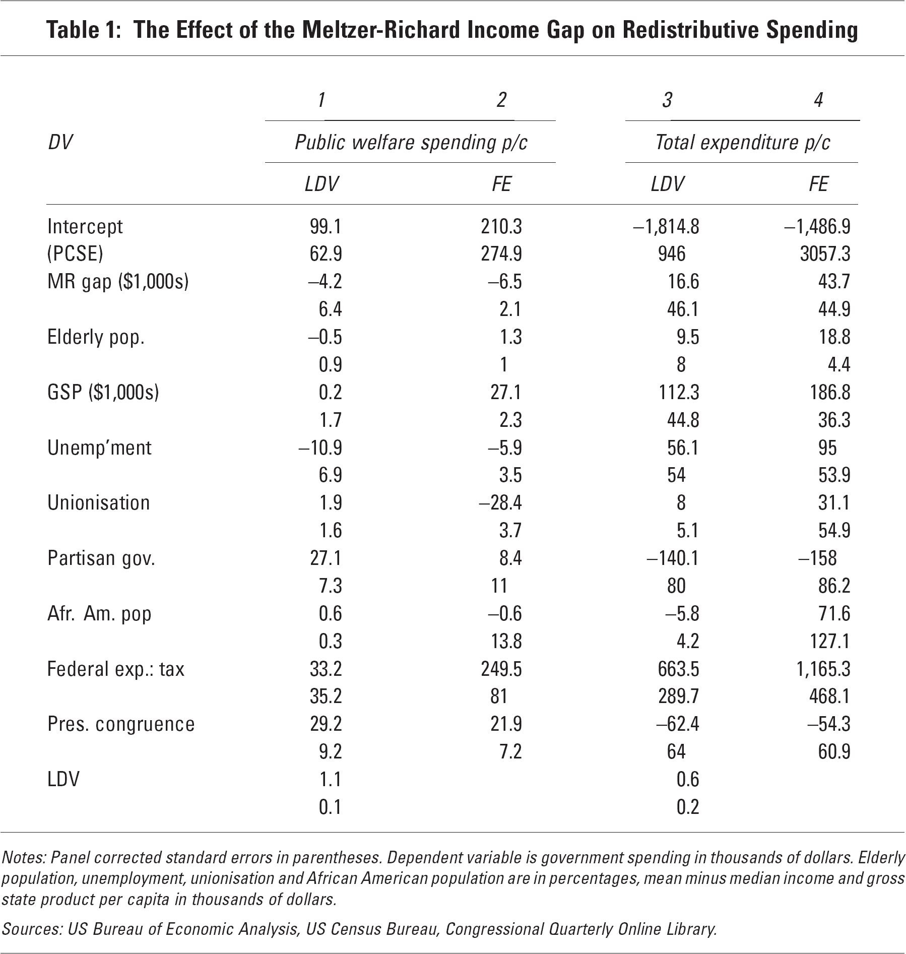
Notes: Panel corrected standard errors in parentheses. Dependent variable is government spending in thousands of dollars. Elderly population, unemployment, unionisation and African American population are in percentages, mean minus median income and gross state product per capita in thousands of dollars.
Sources: US Bureau of Economic Analysis, US Census Bureau, Congressional Quarterly Online Library.
For the other three specifications, the impact of the median voter's income shortfall is negative, contrary to theoretical prediction but consistent with some of the other findings in the literature. Considering fixed effects models of public welfare spending, and either specification for overall spending, I find evidence of the ‘Robin Hood paradox’ whereby greater inequality leads to lower levels of redistribution. However, again these effects are very small in substantive terms: the $1,000 change in median voter income shortfall (which represents a change of about one-fifth of a standard deviation of that variable) leads to a change of $40–$60 in absolute per capita dollars of total spending (2 to 4 per cent of the dependent variable's standard deviation). The fixed effects model for public welfare implies a statistically significant but substantively tiny $8 change in redistribution. Thus overall the empirical results indicate that the impact of the median voter's income on redistribution is substantively small regardless of how we measure it, or in which direction it affects outcomes. Given the weight that is at least implicitly given to the relative income of voters in the literature, this is a surprising and important null finding.
Since the models are specified to examine the effects of the income gap, rather than to examine the impact of the control variables, I will not discuss them at length. Nevertheless, they perform generally as would be expected, if somewhat inconsistently across specifications, with the exception of the variable for partisan congruence which appears positively signed for public welfare expenditures, but negatively for total expenditures. To the extent that earmark spending (which would appear in the latter dependent variable but not the former) can be expected to be more susceptible to partisan manipulation at the federal level, this is somewhat surprising.
More interesting than the control variables (and potentially more problematic for interpreting the results) is the discrepancy between the lagged dependent variable and fixed effects models for public welfare. Notwithstanding that both are substantively small effects, the lagged dependent variable model estimates a statistically significant positive effect of the income gap on public welfare spending, while with fixed effects the estimate is negative and, again, statistically significant. This difference can be better understood by differentiating between variation within states (over time) and variation between states (Bartels, 2010). Decomposing this variation (not shown) indicates that, between states, this inequality measure does have a positive association with public welfare spending; however, the association within states over time is negative. This makes sense of the impact of including fixed effects, as the state dummies parse out the between-state variation.
To examine the robustness of these results to alternative specifications, I also ran models including both the lagged dependent variable and fixed effects (not shown). The results for the variables of substantive interest are close to those from the LDV models. This is consistent with the results of Sven Wilson and Daniel Butler (2007) who find that while the bias of the coefficient on the lagged dependent variable (γ, above) can be large in models including both the LDV and fixed effects, bias on the estimates of β is usually small when both the fixed effects and lagged dependent variables are included (Wilson and Butler, 2007).
Another common approach when dealing with time series cross-sectional data draws on the econometrics of panel data. The generalised method of moments (GMM) (Arellano and Bond, 1991) uses lagged values to instrument for potentially endogenous independent variables, producing unbiased parameter estimates under certain general conditions. However, the complexity of the estimation procedure – particularly as the number of time periods (and thus the number of instruments) gets larger – means that the advantages of this method in terms of consistency may be outweighed by its disadvantages from an efficiency standpoint (Beck and Katz, 2004). For reasons of space I omit the presentation of these results, but they largely bear the same substantive interpretation as the LDV models in Table 1, with even smaller point estimates that generally do not reach statistical significance.
It might also be argued that the aspect of redistribution that is likely to be influenced by electoral politics and the preference of the median voter is the effort that the government makes to redistribute, relative to the resources of the state, rather than its absolute levels (since poor states may simply be less able to afford extensive redistribution). Thus I also consider redistributive spending per capita relative to state product. The results for these measures closely parallel those for the dollar per capita measures: the Meltzer-Richard prediction of a positive point estimate of the median voter income shortfall is borne out in the LDV model for public welfare spending, but the ‘Robin Hood paradox’ is in evidence in the other three model specifications. While the substantive interpretations are a little less straightforward in this case (the coefficient reflecting an increase in the share of GDP per capita that is committed to redistribution) the estimated effects are again substantively small.
The results for the income of the median voter thus provide little support for the theoretical predictions of the median voter-based theories.
If there is little evidence of a large substantive effect of the income gap from the mean to the median voter, what are the implications for interpreting the impact of inequality and turnout on redistribution? I estimate a set of models in which both of these variables are included, and introduce the median voter's income as a covariate. If the impact of these macro-level variables is as the micro-logic of the model claims (via the income of the median voter), then the inclusion of these controls should diminish the direct effect of turnout and inequality, as the effect should be picked up by the median voter income parameter. Table 2 shows the results of this analysis.
The Impact of Median Voter Mechanisms on Redistributive Spending
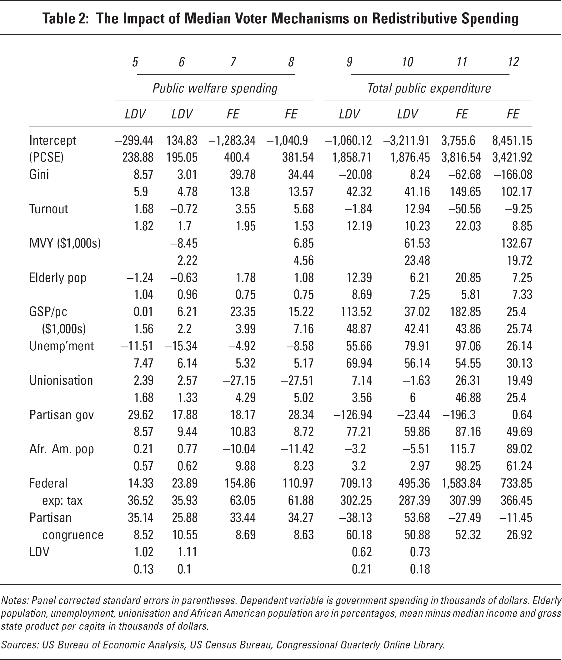
Notes: Panel corrected standard errors in parentheses. Dependent variable is government spending in thousands of dollars. Elderly population, unemployment, unionisation and African American population are in percentages, mean minus median income and gross state product per capita in thousands of dollars.
Sources: US Bureau of Economic Analysis, US Census Bureau, Congressional Quarterly Online Library.
The key take-away point from Table 2 is the absence of any consistent effect of incorporating direct measures of median voter income on the coefficients for inequality and turnout. The estimated coefficients in models 6, 8, 10 and 12 which include the median voter's income as a control are always within one standard error of their counterpart estimates in the odd numbered models that do not include median voter income. As well as being statistically indistinguishable from zero, the impact of including the direct measure of median voter income has an inconsistently signed effect on the estimates for inequality and turnout – increasing the slope of the association with turnout in three of the four cases (counter to the implications of conventional intuition). This basic result is robust across alternative specifications (GMM models, models including both lagged dependent variables and fixed effects, and across ‘effort’ measures of spending relative to gross state product), as well as different lag structures for the independent variables. These models do indicate a positive effect of inequality at least on public welfare expenditure, but do not replicate the finding in the literature that higher turnout is associated with higher spending on either measure. This suggests two interesting questions. First, by what mechanisms does inequality affect redistribution? Second, what determines the income of the median voter and the gap between median voter and average income? It is to this latter question that I now turn.
First, consistent with the conventional wisdom and indeed with intuition, higher inequality is associated with a bigger gap between median voter income and average income. Surprisingly, however, the overall level of turnout has little consistent effect. Thus it appears that there is enough variation in the distribution of voting and non-voting across the income distribution (across states) to make the relationship between turnout and voting outcomes more complicated. Table 3 (models 13–16) presents ordinary least squares models regressing the ‘Meltzer-Richard income gap’ on inequality, turnout and control variables. Since all of these variables are elements of the economic structure, I use contemporaneous measures of the dependent and independent variables to probe their covariation. This analysis should be seen primarily in descriptive terms rather than interpreted causally. Models 17–24 provide analogous lagged dependent variable and fixed effects models for those more interested in a causal interpretation, but for reasons of space the discussion here will focus on the simple correlations.
Determinants of the ‘Meltzer-Richard Inequality’ Income Gap
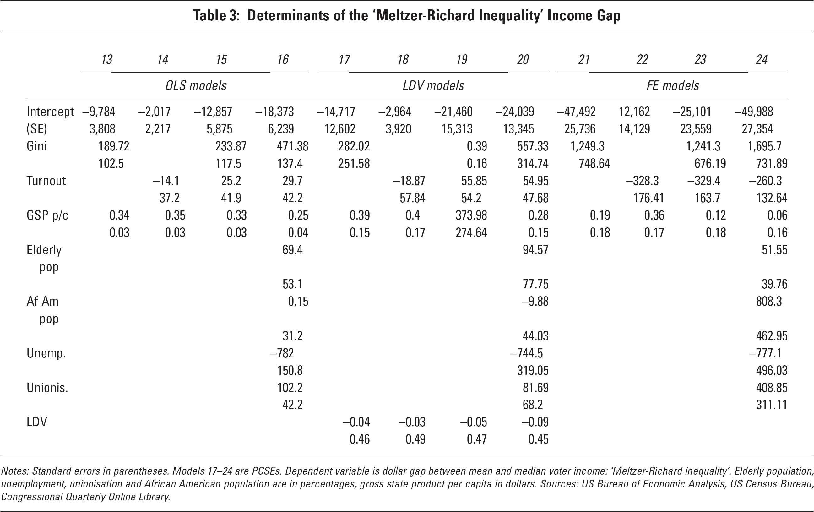
Notes: Standard errors in parentheses. Models 17–24 are PCSEs. Dependent variable is dollar gap between mean and median voter income: ‘Meltzer-Richard inequality’. Elderly population, unemployment, unionisation and African American population are in percentages, gross state product per capita in dollars. Sources: US Bureau of Economic Analysis, US Census Bureau, Congressional Quarterly Online Library.
Models 13, 14 and 15 regress the income gap on inequality, turnout and both these variables, respectively, with only gross state product as a control variable (since the income gap measure is an absolute dollar value measure). To recap, we would expect to see both higher inequality and higher turnout having a positive association with the income gap, the latter by incorporating more of the poorer voters into the measure as turnout increases. And indeed that pattern does play out for inequality: a higher Gini coefficient translates to a higher income gap. For turnout, though, the simplest relationship (model 14) in fact shows a slight negative relationship. But since high turnout states also tend to be less unequal, the baseline results need to incorporate both these variables (model 15). Here still, in contrast to the results across countries in Mahler (2008), these data do not show a strong relationship between the level of turnout and the income skew in turnout.
While this association – or lack of it – might seem paradoxical, once turnout falls below full participation, differences across states in the way that abstention is distributed may complicate the relationship between income skew and turnout. In this case, variables that might be associated with differences in who is likely to abstain, across states, may also be important in determining the gap between the median voter and average income. For example, if the elderly tend to be poorer than average, but to vote at higher rates, then we would expect that states with a high proportion of elderly people would have lower median voter income at any level of turnout, since those who are voting are more likely to be poor. To the extent that unions mobilise low-income political participation, the same logic would apply. Both these variables, then, would be expected to be associated with a larger income gap. Evidence that the socio-economic gradient in voting is less pronounced among African Americans than among white Americans (Jaynes and Williams, 1985; Radcliffe and Saiz, 1995) would imply that the share of African Americans in the population would have a similar effect. Unemployment, by contrast, can be expected to work in the opposite direction, as the unemployed are likely to be poor, but also are more likely to be disengaged from political action. Thus unemployment rates would be expected to be negatively related to the income gap, as the more of the poor who are unemployed, the fewer of them will vote.
All of these associations are found in the data, although the relationship between the income gap and the elderly and African American population shares are weak. States with higher unemployment do have lower median voter income gaps, other things being equal, and more highly unionised states have higher gaps. Thus these descriptive models provide a way of making sense of the lack of a relationship between turnout levels and income skew in the US states. In turn, this helps explain the absence of a strong relationship between turnout and redistributive policy in Table 2, and the fact that including controls for the income of the median voter changes this so little.
Conclusions
In conclusion then, the hypothesised micro-logic that relates inequality and turnout to government spending is not corroborated by measures that consider the individual-level parameters directly, as opposed to relying on jurisdiction-level aggregates. The gap between the income of the median voter and average income has, if anything, a negative impact on redistributive spending. However, while precisely estimated from a statistical standpoint, this effect is very small. Thus from a substantive viewpoint, the key finding is one of little effect of this type of inequality on redistribution. Within the US states in the period in question, the Meltzer-Richard model finds little support.
The implications of the data are broader than just the Meltzer-Richard model, however, as many arguments linking voter turnout to redistributive outcomes rely implicitly on a mechanism that runs via the income of the median voter. The second finding of this article is that the income of the median voter does nothing to mediate the impact of turnout on redistribution. Indeed, I find little evidence that turnout has an important impact on redistribution at all. Equally (and in line with the negative impact of inequality found above) to the extent that the income of the median voter matters for spending outcomes, it is richer median voters, rather than poorer ones, who demand higher redistribution.
Finally, I explore the relationship between the median voter's income gap and turnout, to understand better the lack of impact that turnout has on redistribution. In contrast to Mahler (2006), but consistent with other results in the literature (Hill and Leighley, 1992), the data from the United States indicate that turnout and income skew are not very closely tied. This discrepancy is perhaps understandable in light of the different scale of variation in terms of turnout: where a decrease in turnout is from 100 to 80 per cent, it obviously introduces the potential for class bias where none would otherwise exist. However, where variation in turnout is around on average a little over 50 per cent, there is no such necessary implication for lower turnout. In fact, other factors such as unemployment and unionisation levels in particular appear more closely related to changes in the income gap, a logic understandable in terms of the role of these variables in supporting or undermining the political engagement of the poor which may be more direct than turnout itself.
Footnotes
This research was funded in part by Harvard's Doctoral Fellowship on Inequality and Social Policy and by the Marie Curie Excellence project in Political Economy (POLGLOBALSERV) at Trinity College, Dublin. I would like to thank Jim Alt, Ben Goodrich, Peter Hall, Michael Henderson, Torben Iversen, Christopher Jencks, Michael Kellerman, Jonas Pontusson, Thomas Romer, Daniel Schlozman and Theda Skocpol for comments on earlier drafts; all remaining errors are my own.
1
Analyses available on request.