
Abstract

Killeen (2005) recommended replacing the p values of significance tests with replication probabilities, which he determined as follows: Assume d
x
, the estimate of the effect size δ in study x, is positive and its sampling error, e
x
=d
x
−δ, is normally distributed with mean 0 and variance σ2, that is, N(0, σ2). It follows that the effect size in a replication, d
y
= (δ+e
y
), can be rewritten as (d
x
−e
x
+e
y
), where e
y
is the replication sampling error. Consequently, d
y
is distributed as N(d
x
, 2σ2), because d
x
is a constant and e
x
and e
y
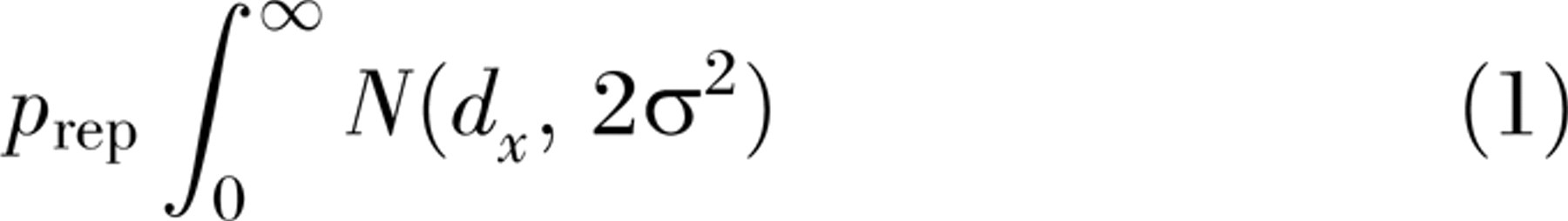
are independently distributed as N(0, σ2). The replication probability (p
rep), the probability that d
y
> 0, can now be found by integrating the distribution of d
y
(see Killeen's Equation 1):
No reference to δ appears in the calculation; nevertheless, a distribution has implicitly been attributed to δ. Consider the replication probability based on n identical replications yielding effect sizes d
y
, d
y
, d
y
, …, d
y
with errors ey1
, ey2
, ey3
, …, eyn
, each independently distributed as N(0, σ2). The combined effect size is the mean of the d
y
s (d̄
y
), which is distributed as N(δ, σ2/n). An analogous argument leads to the conclusion that

WHAT IS WRONG WITH FIDUCIAL PROBABILITIES?
In any attempt to compute replication probabilities, information concerning the population effect size distribution needs to be taken into account. Imagine a researcher who tested only true null hypotheses (e.g., randomized control trials testing the existence of supposed supernatural phenomena that did not exist). In this case, given standard assumptions and discounting effect sizes of 0, the replication probabilities would equal .5. Admittedly, this example is an idealization, but studies differ in what is known about the effects they test, and replication probabilities should reflect this. Indeed, any simulation of replication probabilities has to incorporate a distribution for δ. Killeen's approach ignores such distributions and as a result seems appropriate only when there is no relevant prior information.
Fisher's fiducial argument was similarly based on taking prior information to be irrelevant, but it has not stood the test of time (Seidenfeld, 1992; Zabell, 1992). The problem with fiducial inference is that the probability of δ depends on how the prior ignorance of δ is characterized. Seidenfeld associated the problem with representing ignorance of a parameter by a uniform distribution, and Lindley (1958) argued that in the one-parameter case, the fiducial argument is either inconsistent or equivalent to a Bayesian argument with a uniform prior. However, when a uniform prior is assumed, ignorance of δ and ignorance of any one-to-one function of δ result in different prior probability distributions despite the ignorance being the same in each case. In addition, unbounded uniform priors are not proper probability distributions, as their integrals over all possible values do not equal 1. Indeed, the posterior distribution N(d x , σ2) cannot be obtained using any genuine prior probability distribution (O'Hagan, 1994, p. 77). O'Hagan recommended that the use of improper priors be restricted to situations in which all “reasonable” priors would result in posterior distributions that did not differ greatly from each other (p. 111).
Returning to Killeen's argument, it seems to result in the following paradox. Before d x is observed, there can be information concerning the likely values of δ and d y , yet after d x is observed, such prior information is irrelevant because δ is distributed as N(d x , σ2) and d y is distributed as N(d x , 2σ2). In the case of d y , this follows because, as stated earlier, once d x is known, it is assumed that d y =d x −e x +e y , where d x is a constant and both error terms are independently distributed as N(0, σ2). However, the previously mentioned example concerning the investigator of supernatural phenomena contradicts this characterization of the uncertainty after d has been observed. Here the prior distribution of δ is δ= 0 with p= 1, and if d x is found to be c, then e x also equals c with a probability of 1. Thus, e x is not distributed as N(0, σ2), as Killeen supposed. The point is that once d x is known, the uncertainty regarding e x should be given by its probability distribution conditioned on the observed value of d x . This conditioning process incorporates the prior distribution of δ into the calculation of both the distribution of replication probabilities and the posterior probability distribution of δ.
CONCLUSIONS
As the adage has it, “when something looks too good to be true, it probably is.” If it were possible to compute replication probabilities ignoring everything but the data, then these probabilities would be “objective” and could form the basis of an alternative to significance tests. Unfortunately, this is not possible. To find a replication probability from d x , one needs to know both the probability law generating d x and the prior probability distributions of the law's parameters. A problem exists because complete ignorance of a parameter does not seem equivalent to any prior, but this is just an example of the more general principles that probability models only approximate people's uncertainties (Macdonald, 2002) and that statistical inferences are not entirely based on logic (Macdonald, 2004). Seidenfeld (1992) summarized the case against fiducial probabilities by quoting Savage (1961, p. 578), who said that to make the Bayesian omelet, you have to break the Bayesian eggs.