
Abstract
We study a supply chain where an original equipment manufacturer (OEM) buys subassemblies, comprised of two complementary sets of components, from a contract manufacturer (CM). The OEM provides a demand forecast at the time when the CM must order the long lead‐time set of components, but must decide whether or not to provide updated forecasts as a matter of practice. Forecast updates affect the CM's short lead‐time purchase decision, and the anticipation of updates may also affect the long lead‐time purchase decision. While the OEM and CM both incur lost sales costs, the OEM can decide whether or not to share the overage costs otherwise fully borne by the CM. We investigate when the OEM is better served by committing to provide updated forecasts and/or committing to share overage costs. For a distribution‐free, two‐stage forecast‐update model, we show that (1) the practice of providing forecast updates may be harmful to the OEM and (2) at the OEM's optimal levels of overage risk sharing, the CM undersupplies relative to the supply chain optimal quantity. For a specific forecast‐update model, we computationally investigate conditions under which forecast updating and risk sharing are in the best interest of the OEM.
1. Introduction
Firms may outsource manufacturing operations for a variety of reasons. While outsourcing could presumably reduce the direct cost of an item being produced on behalf of the original equipment manufacturer (OEM), it also introduces other costs related to the need to coordinate with the contract manufacturer (CM). Motivated by discussions with OEMs and CMs in the computing equipment industry, we investigate the setting where an OEM hands over sub‐assembly or finished product manufacturing as well as component procurement to a CM. This scenario is consistent with the turnkey setting described in the recent typology of OEM–CM outsourcing relationships offered by Amaral et al. (2006). In this setting, an important question is, “What tools or incentives can the OEM use to ensure that the CM acts in the best interest of the OEM, but that also ensure that the CM receives some mutual benefit?” Here, we investigate two interrelated tools an OEM may use to influence CM behavior: the sharing of component inventory risk and providing ongoing access to updated demand forecasts.
Our conversations with practicing managers at OEM and CM firms indicate that the risk of component overage is an area of significant concern to both parties. The CM does not want to be left holding expensive, potentially obsolete component inventory if the OEM's forecasts turn out to have been overly optimistic. On the other hand, the OEM is cognizant of the fact that the CM, concerned about this inventory risk, might underbuy components relative to the demand forecast, purchasing enough components to support only a fraction of the forecast. Recent research provides empirical evidence for this kind of forecast gaming and its effects in the semiconductor manufacturing equipment industry (Terwiesch et al. 2005), and recent modeling work (Özer and Wei 2006) demonstrates the value of capacity commitments from a customer as a means for a manufacturer/supplier to extract truthful forecast information from the customer. Interestingly, a CM with whom we spoke indicated that their contracts with OEMs explicitly require them to, in good faith, commit to pursuing a supply of components that sufficiently supports the demand forecast passed to the CM by the OEM. The onus on the OEM in these arrangements, however, is that the OEM provides a contractual commitment to the CM that it will pay inventory‐related costs that stem from obsolete or excess conditions created by OEM demand forecasts. In this particular case, the burden is on the CM to prove the level of inventory that is obsolete or in excess by maintaining a precise account of the rolling forecasts and the matching component purchases.
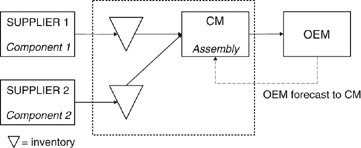
In most production systems, components that are part of a larger assembly commonly have different lead times. Typically in this situation, a manufacturer would order each component at the latest possible time that allows the component to be available for planned production. Motivated by the OEM–CM forecasting, procurement, and production relationships described above, we explore the simplest setting of this problem, in which a product composed of two components that have different lead times is produced to meet a random demand in a single selling period. New information about product demand may be gathered in the period between the resupply lead times of the two components. The supply chain that is the object of our research is depicted in Figure 1. In this supply chain, an OEM uses a CM to assemble a semi‐finished product that is customized by the OEM into a finished product. The CM uses an assemble‐to‐order system and is responsible for the procurement of both components. All components unused at the end of the selling season are salvaged by the CM. Our baseline model of the OEM–CM interaction assumes that the OEM bears no risk for component overage, and bears only the risk of insufficient finished product supply. Thus, the OEM certainly would prefer that the CM keep high inventory levels for both components so that he will not forfeit any sales opportunities.
It is common in high‐tech manufacturing for an OEM to negotiate a cost‐plus contract with a CM. Margins for these contracts are typically low due to fierce competition. As with simpler, one‐stage buyback or revenue‐sharing models, if the OEM in our model could set the CM margin (by setting the wholesale price) and offset CM risk, he could set the margin close to zero and absorb nearly all of the risk, driving CM profit arbitrarily close to zero. So, the fixed CM margin we assume in our model can be thought of as the smallest margin the OEM is able to force on the CM. Since the purpose of this research is to investigate the impact of sharing inventory risk and providing forecast updates, we do not address the market price‐setting problem of the OEM. Thus, both CM and OEM margins are exogenous in our model. Interactions between pricing decisions and the forecast‐update and risk‐sharing decisions that we study here may, however, be an interesting topic for future research.
We assume that, although the OEM in this supply chain has ceded the authority for component ordering decisions to the CM, the OEM can influence the CM's decisions through two mechanisms: (1) providing (or not providing) demand forecast updates and (2) offering contract terms to the CM whereby the OEM assumes some fraction of the CM's overage cost, a control mechanism we call a risk‐sharing agreement. Risk in this context refers to the risk of excess component inventory, not risk preferences of either decision maker. We assume throughout that both the CM and OEM are minimizing expected costs.
The primary questions we address in this research focus on performance from the OEM perspective. Specifically, we seek to answer the following questions:
Under what conditions is it beneficial for the OEM to provide updated demand forecasts as a matter of practice? Under what conditions should the OEM offer to share component overage costs with the CM? How do the forecast updating and component overage sharing decisions interact? How do the OEM's decisions affect the CM and the supply chain as a whole?
To answer these predominately OEM‐centric questions, we must understand the CM's problem in isolation—the problem inside the dashed box in Figure 1, which we call the two‐component newsvendor problem. The distinguishing aspect of this problem is that two complementary components with different lead times must be purchased under demand uncertainty regarding the product into which they are assembled. Assume without loss of generality that component 1 is the long lead time component. After committing to some component 1 quantity, the CM may have access to an updated forecast when it is time to purchase component 2. With a forecast update the CM might buy component 2 in a quantity less than her already committed purchase quantity of component 1; otherwise, she will order component 2 in a quantity to match the quantity of component 1. Furthermore, the anticipation of the forecast update will affect the CM's component 1 decision. Understanding how the CM will react to both the expectation as well as the receipt of the forecast update is critical to understanding the OEM's ability to affect supply chain performance through forecast updating and risk sharing.
The rest of this paper is organized as follows. After reviewing related literature in Section 2, we formulate the problem in Section 3, first using a general, distribution‐free forecast‐update model. Under this general model, we demonstrate that forecast updating can hurt OEM performance whether the OEM is choosing to share component risk or not. Furthermore, at optimal risk‐sharing levels, the CM underproduces relative to the supply‐chain‐optimal solution; that is, this style of component risk sharing cannot completely coordinate the supply chain. A specific forecast‐update model is presented in Section 4. For this specific model, we show that it is in the OEM's best interest to provide forecast updates. We then use the model to computationally investigate conditions under which the OEM benefits by updating forecasts and/or sharing component overage risk. Concluding remarks are offered in Section 5.
2. Related Literature
Before reviewing the literature related to the problem we study, let us first point out the manner in which our research stands apart. First, much of the literature we review below considers ordering or producing a single item at two or more instants under a wholesaler–retailer context. By contrast, we consider a contract manufacturing setting that concerns ordering decisions for complementary components with different lead times. There is some prior work on optimal ordering policies for multi‐component assembly systems (e.g., Gerchak and Wang 2004, Gurnani et al. 1996, 2000, Kumar 1989). Most of this work, however (Gerchak and Wang excepted), takes a different perspective than ours, treating supplier yield as an exogenous input and not incorporating the possibility that supplier and customer incentives could be aligned to mutual benefit. In a vein similar to ours, Gerchak and Wang (2004) consider decentralized coordination schemes, but among multiple suppliers of a single, common customer, and without the possibility of forecast updates. In addition, in our work, many of the analytic results are developed using a distribution‐free forecast‐update paradigm rather than one based on the normal distribution as in previous research (e.g., Ferguson et al. 2005, Fisher and Raman 1996, Gurnani and Tang 1999, Miyaoka and Hausman 2007).
Substantial research efforts have been directed to inventory and/or production planning decisions that account for updated demand information. Examples of this work date from the 1960s (e.g., Hertz and Schaffir 1960, Murray and Silver 1966), through the 1970s and 1980s (e.g., Chang and Fyffe 1971, Crowston et al. 1971, Hausman and Peterson 1972, Bitran et al. 1986), and to recent decades (e.g., Bradford and Sugrue 1990, Eppen and Iyer 1997, Lovejoy 1990, Weng and Parlar 1999). This line of research assumes that demand or information variables follow a known distribution with unknown parameters, poses initial estimates of those parameters from historical data, and uses updated information to revise the parameter estimates between key decision points to improve production and/or inventory decisions. In addition, researchers have begun to explore the complexities of the forecasting process and the effects of human judgment, biases, and gaming on generating forecasts and future updates to them—e.g., Terwiesch et al. (2005), mentioned above, and more recent research from Oliva and Watson (2008), whose case‐study work documents the organizational challenges of accurately incorporating new information in updated forecasts.
Although the modeling research discussed above, extending from the 1960s forward, addresses demand forecast updates, it does not consider coordination of the incentives of independent firms in a decentralized supply chain, a modeling issue whose importance is clearly highlighted by the recent empirical work of Terwiesch et al. (2005) and Oliva and Watson (2008). A great deal of work has been done in the realm of supply contract design and channel coordination, primarily in a single‐product context. Cachon and Lariviere (2001) present a model that serves as a broad modeling framework for various buyer–supplier contracting work that ultimately can be traced back to the seminal work of Pasternack (1985), although they consider the downstream partner to be the one that sets the contract terms, which is consistent with our model and with that of Ferguson et al. (2005), discussed below. Tsay et al. (1998), Lariviere (1998), and Cachon (2003) present comprehensive reviews of this literature.
Recent work that combines the impact of forecast updates and/or forecast sharing with channel coordination issues includes Donohue (2000), Ferguson et al. (2005), Mishra et al. (2008), Miyaoka and Hausman (2004), and Miyaoka and Hausman (2007). Donohue (2000) demonstrates the existence of wholesale prices and return prices that achieve supply chain optimality under a distribution‐free model, and also shows that the pricing conditions for optimality vary depending on the extent of information revealed between forecast updates. Ferguson et al. (2005) consider recourse‐based ordering policies in a model that allows an end‐product manufacturer to provide multiple information updates to its component supplier. Mishra et al. (2008) study a situation that reflects issues considered by both Donohue and Ferguson et al., but where both the manufacturer and the customer generate different (although possibly correlated) forecasts of demand. They study the impact of various levels of forecast uncertainty and correlation on the optimal retail and wholesale prices, and on manufacturer and retailer profits in a game‐theoretic setting. Both papers by Miyaoka and Hausman investigate the impact of providing updated demand forecasts in decentralized supply chains. The first of these papers shows that non‐updated demand forecasts may actually result in better operating performance in a dynamic setting where new information would otherwise cause undesirable changes in production planning. The second paper focuses on the impact of updated forecasts on capacity commitments by a supplier. This work is similar in spirit to our research in that we also investigate situations where providing updated demand information in a decentralized setting can degrade overall performance. Our work is differentiated by the complementary component structure and a different forecast update mechanism.
3. General Model
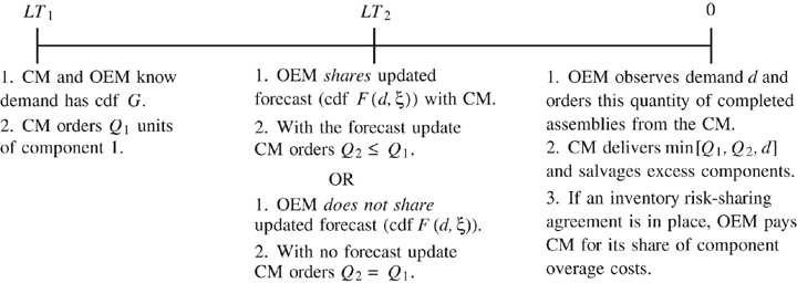
As described in Section 1, the OEM in our model sells to its clients a final product, which is built from a semi‐finished item supplied by the CM. In order to manufacture products for the OEM, the CM must order two components that have different lead times. The CM uses an assemble‐to‐order system and is responsible for the procurement of both components. All components unused at the end of the selling season are salvaged by the CM based on market‐determined salvage values. Let LT 1 and LT 2 be the lead times for components 1 and 2, respectively. For convenience, we count down in time from LT 1, when component 1 is ordered, to 0, when random demand D is realized. The sequence of events is depicted in Figure 2; details of the forecast update regime and the inventory‐risk‐sharing agreement are discussed below. Generally, the CM buys Q 1 units of component 1 at time LT 1, then Q 2 units of component 2 at time LT 2. At time 0, the OEM observes demand d and places an order with the CM equal to demand. The CM delivers the minimum of this order and the potential supply, min[Q 1, Q 2, d]. We assume without loss of generality that the sum of unit purchase costs for the two components is 1 with per‐unit salvage losses for components 1 and 2 given by l 1 and l 2, respectively (i.e., l i is the unit cost minus the salvage value). The CM charges a wholesale price of 1+m c to the OEM, and the OEM's selling price is 1+m o +m c ; thus, m c is the CM's profit margin and m o is the OEM's margin.
As we discussed at the outset of the paper, OEM–CM contracts with which we are familiar imply some liability on the part of the OEM to compensate the CM for excess inventory that was created by the CM's actions to procure components in support of the OEM's forecast. We model the level of OEM liability directly as a fraction of the component overage cost that the OEM agrees to pay as part of the terms of the contract. Specifically, the OEM absorbs a fraction, γ i (0≤γ i ≤1), of the salvage loss l i of each unused component i.
Our forecast‐update framework operates as follows: between LT 1 and LT 2 the OEM observes some information (e.g., general state of the economy, industry trends, updates from the sales force) that permits an updated demand forecast at time LT 2. Let ξ, with pdf h, represent the realized value of the information that affects the forecast, and let F(·, ξ) be the cdf of demand, conditionally defined on ξ. Let G be the cdf of demand at time LT 1. We obtain G from F(·, ξ) using the law of total probability. We place no restrictions on the set of conditional distributions F(·, ξ), such as countability of the elements or having all the elements belong to the same family of distributions. As such, the bivariate normal update framework in, among others, Fisher and Raman (1996) and the additive‐normal framework in Ferguson et al. (2005) and Miyaoka and Hausman (2007) are contained as special cases of this framework.
So, the OEM must decide (1) whether to provide a forecast update to the CM or not and (2) the extent to which to share overage risk with the CM. To optimize, the OEM must find the best risk‐sharing parameters, γ 1, γ 2, under both forecast‐update and no‐forecast‐update regimes and compare the two results. For each of these regimes, we first develop the CM's decision problem for fixed γ 1, γ 2. Assuming the CM will choose component purchase quantities to minimize cost, we can then formulate the OEM's problem of selecting γ 1, γ 2 to minimize his cost.
In the sections that follow, we will compare the performance of this decentralized system with the centrally planned supply chain optimal solution. As we demonstrate below, one easily obtains the total cost and optimal solution for the overall supply chain by using the cost function developed for the CM, but replacing the CM's margin and component losses with those for the overall supply chain.
3.1. OEM Does Not Provide a Forecast Update to the CM
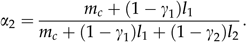
When the OEM does not provide a forecast update to the CM, the CM will buy components in equal quantities. She faces a standard newsvendor problem with shortage cost m
c
and overage cost (1−γ
1)l
1+(1−γ
2)l
2. The CM would choose cost minimizing quantities 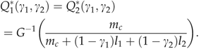
In selecting values of γ
1, γ
2, the OEM determines what share of overage cost he will absorb, influencing the CM's critical fractile. The OEM then chooses values of γ
1, γ
2 to minimize 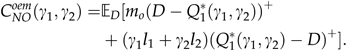
We use the subscript NO to denote the no‐forecast‐update case. Below, the subscript UP will denote the case where forecast updates are provided.
3.2. OEM Provides a Forecast Update to the CM
If the OEM provides a forecast update to the CM, the order quantities for the two components may differ since the CM can take advantage of the new information in making her component 2 purchase decision. To construct the CM's cost function, we first determine the component 2 decision conditioned on the component 1 order quantity (Q
1) and the forecast update (F(·, ξ)). At this point in time (LT
2), the CM solves a newsvendor problem with overage cost (1−γ
2)l
2. The underage cost is m
c
+(1−γ
1)l
1 since having one additional component 2 when demand exceeds supply would result in meeting a sale and putting to use a component 1 that would otherwise have been salvaged. We call this critical ratio (at time LT
2) 
In addition, we define the quantity that the CM would like to buy, if not constrained by the choice of Q
1, as β(ξ)=F
−1(α
2, ξ), from which it follows that the optimal component 2 order (conditioned on ξ)  . It is easy to show that the optimal cost for this problem—a standard newsvendor problem—is convex in the constraint determined by Q
1. Furthermore, the expectation operator preserves convexity; so this problem is also convex in Q
1.
. It is easy to show that the optimal cost for this problem—a standard newsvendor problem—is convex in the constraint determined by Q
1. Furthermore, the expectation operator preserves convexity; so this problem is also convex in Q
1.
Now, assuming that the CM will order Q
2 optimally at time LT
2, we formulate the CM's cost as a function of the component 1 decision Q
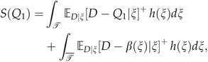
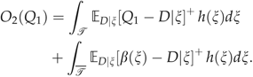
1. The CM's cost function has three components: expected shortages, S(Q
1), and expected component overages O
1(Q
1), O
2(Q
1). In developing these expressions below, we develop separate terms for the cases where the CM chooses to match component orders (Q
1=Q
2) and where she chooses to buy Q
2<Q
1. Define  to be the set of realizations of the update random variable, for a given value of Q
1, where the CM matches component orders,
to be the set of realizations of the update random variable, for a given value of Q
1, where the CM matches component orders,  . We will also use the complement of this set,
  .
. 
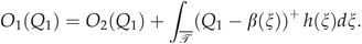
The overage of component 1 is equal to the overage of component 2 plus Q
1−Q
2, the number of component 1 units that are orphaned by the choice of Q
2. 
With these expressions, and assuming optimal ordering at LT
2, the CM's expected total cost as a function of Q
1 can be stated as 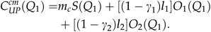
The following proposition characterizes how shortages and component overages are affected by the CM's choice of Q
1 and by the value of α
2, the critical fractile that determines Q
2. We examine α
2 rather than  noting that for any Q
1 and forecast update F(·, ξ),
noting that for any Q
1 and forecast update F(·, ξ),  is non‐decreasing in α
2. Proofs are in Appendix A.
is non‐decreasing in α
2. Proofs are in Appendix A.
P
It is intuitive that shortages are non‐increasing and component overages are non‐decreasing in Q 1, and component 2 overages are non‐decreasing in α 2. The fact that overages for component 1 are non‐increasing in α 2 is explained by the fact that a larger α 2 equates to the CM buying more of component 2. By buying more of component 2, the CM increases the chance that a component 1 will be assembled and sold rather than left over.
Next we investigate the effects of the CM's optimal decisions on the OEM's cost function. As noted above, the CM's problem is convex in Q
1, so there is a unique optimal value of Q
1. In addition, it is evident that the OEM's choices of γ
1, γ
2 will affect the CM's optimal choices of Q
1 and Q
2, where the Q
2 choice is conditional on the Q
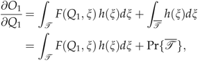
1 choice and the forecast update. Assuming that the CM orders both components optimally, we can define  to be expected shortages and overages. The OEM's cost function is
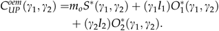
For the same risk‐sharing agreement, the CM will always prefer receiving the forecast update. (She could, of course, ignore the update and do no worse.) For the OEM, however, the situation is not immediately clear. Note that with γ 1=γ 2=0, the OEM's cost function is comprised solely of the cost of shortages. While one might suspect that providing the forecast update would reduce shortages, this need not be the case. We offer the following observation.
O
In Section 4, we prove that additional demand forecast information will in fact reduce shortages for a specific forecast‐update model. For now, however, consider the following example that demonstrates that shortages can increase with a forecast update at LT
2. Assume the (updated) demand distribution at LT
2 will be one of the following two situations: (1) either 1 or 2 with probability 2/3 or 1/3, respectively; (2) exactly 3 with probability 1. If situation (1) occurs with probability 3/5, the demand distribution at LT
1 is 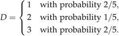
Consider cost parameters of l
1=0, l
2=1, and m
c
=2−ɛ with some small ɛ>0. If the forecast update is not shared, the CM will face a critical fractile of (2−ɛ)/(3−ɛ) and choose  (since P[D≤3]≥(2−ɛ)/(3−ɛ)). This decision clearly results in no shortages. If the forecast update is provided, Q
1
*=3 since there is no salvage loss associated with component 1. At LT
2 the CM will choose Q
2
* based on α
2=(2−ɛ)/(3−ɛ), implying Q
2
*=1 for situation 1 and Q
2
*=3 for situation 2. This will result in an expected shortage of 1/5, demonstrating that providing the forecast update can increase expected shortages.
(since P[D≤3]≥(2−ɛ)/(3−ɛ)). This decision clearly results in no shortages. If the forecast update is provided, Q
1
*=3 since there is no salvage loss associated with component 1. At LT
2 the CM will choose Q
2
* based on α
2=(2−ɛ)/(3−ɛ), implying Q
2
*=1 for situation 1 and Q
2
*=3 for situation 2. This will result in an expected shortage of 1/5, demonstrating that providing the forecast update can increase expected shortages.
Since we will extend this example later to consider γ 1, γ 2>0, it is worth taking a moment to consider why this scenario permits the observation. Here, there are two update possibilities: demand could be “high” (deterministically 3) or “low” (1 or 2), with no possibilities in between. Many forecast‐update models from the literature, such as bivariate normal and additive normal, discussed above, as well as the uniform–uniform (U–U) model we present below, have update distributions whose means are parameterized by a continuous random variable. That is, they do not allow the update distributions to be far apart, as they are in this example. Or, more precisely, they do not allow a convolved distribution at LT 1 that is bimodal. Such a case may arise, for example, when a new product being launched will be either a hit or a flop. So, one might find, as is the case here, that results that are true when the update possibilities yield a smooth, continuous demand distribution (e.g., that shortages decrease with an update) may not be true when there are a few update possibilities that are quite different from one another.
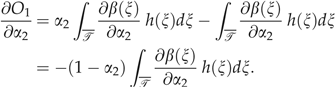
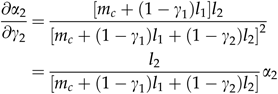
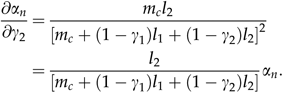
Next, we turn our attention to the general properties of the OEM–CM coordination problem under OEM‐offered risk sharing with the CM. The following proposition describes how the OEM's choices of γ i affect the CM's optimal component 1 quantity, where we let Q 1 *(γ 1, γ 2) be the minimizer of (7), and her optimal component 2 quantity.
P
This result indicates that the OEM can use either γ 1 or γ 2 as a lever to increase the CM's component 1 order quantity Q 1 *; however, increasing γ 1 reduces the CM's component 2 critical fractile α 2. As an immediate consequence of Propositions 1 and 2, we have the following corollary, which partially describes how γi and γ2 affect shortages and component overages.
C
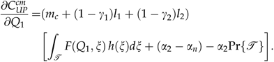
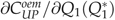
Note that the OEM's contract levers, γ 1 and γ 2, affect the CM's decisions, Q 1 * and Q 2 * (through α 2), but also affect the fraction of the total overage cost absorbed by the OEM. As the following proposition shows, when the OEM chooses γ 1, γ 2 to optimize his cost (Equation [8]), the total supply chain will not be optimized. Before stating the proposition, we note that while we have established that the CM's problem is convex in Q 1, we have not characterized the OEM's problem as convex (or pseudo‐ or quasi‐convex) in γ 1, γ 2. Thus, it is possible for the OEM to have more than one optimal risk‐sharing agreement.
P
This result indicates that even after the OEM employs an optimal risk‐sharing agreement to inflate the CM's procurement decisions, the CM still underbuys component 1 from the overall supply chain perspective. Moreover, we also observe that even when the risk‐sharing agreements are optimized by the OEM, choosing to provide forecast updates to the CM could result in a worse outcome for the OEM.
O
Consider once again the discrete‐demand example from Observation 1 that demonstrated that providing a forecast update can increase shortages. In that example, when there was no forecast update, the OEM faced no shortages and no overage. With the forecast update, however, the CM incurred expected shortages of 1/5. The OEM could offer a small γ 2>0, shifting the CM's component 2 critical fractile such that the CM would chose to have component overages rather than shortages, but even so, the OEM's cost would be strictly positive. Thus, in this case, the OEM is best served by not providing an update.
Proposition 3 implies that, while there is room for a Pareto improvement, such an improvement will not be realized under this risk‐sharing structure. This result is consistent with supply chain coordination results for simpler, single‐product settings such as the buyback setting (see Cachon 2003) where, in addition to a per‐unit adjustment (γ 1, γ 2 in our context), a transfer payment is needed to coordinate the supply chain. The following proposition establishes that there exist values of γ 1, γ 2 that optimize the supply chain.
P
Note that these are not the values that the OEM will choose when optimizing his cost. In fact, if such values were optimal in general, it would contradict Proposition 3, which states that the supply chain is not optimized at the OEM's choices of γ 1, γ 2.
3.3. A Comment Regarding Risk‐Sharing Implementation
The authors' discussions with managers at a computer hardware OEM indicate that there might be some tendency in this particular industry to consider a “γ 1‐only” contract. The reasoning is that, since the long‐lead‐time items are the high‐cost items in this industry, the overage compensation on the low‐cost, short‐lead‐time items would appear to be less important. A means of studying such an approach would be to constrain our problem, forcing risk sharing to be implemented via a “single‐gamma” (SG) contract, where the OEM optimizes over γ 1, but with γ 2=0. Even if a firm were willing to offset risk across both (sets) of components, however, one could also argue that implementation of the most general, “dual‐gamma” (DG) contract might be challenging in practice given that two different contract terms must be negotiated. Thus, one might consider an “in‐between” risk‐sharing arrangement, in which only a single value is specified for both γ variables, i.e., an “equal‐gamma” (EG) contract, which solves the OEM and CM problems by introducing γ in place of both γ 1 and γ 2 in the OEM and CM objective functions.
Note that the analytic results above indicate different effects on key outcomes for the OEM based on changes in γ 1 vs. γ 2. With only a single value of gamma—be that the SG approach of offsetting overage on only component 1, or the EG approach of offsetting overage on both components via a single value of γ=γ 1=γ 2—some of those results may change. In the interest of maintaining brevity and focus in this paper, however, we do not consider those extensions here.
In the following section, we analytically develop a specific forecast‐update model that permits closed‐form solutions for CM and OEM costs and purchase quantities. We develop analytic results for this setting and then use the model to computationally investigate the relative cost benefits to the OEM, CM, and overall supply chain of different forecast‐updating and risk‐sharing strategies.
4. Specific Forecast‐Update Model and Results
4.1. U–U Forecast‐Update Model
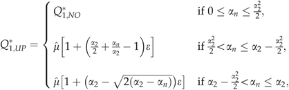
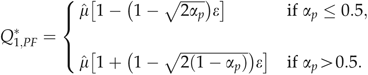
As mentioned above, the bivariate normal forecast‐update model has been the predominant model used in the literature on two‐stage purchasing/production decisions. Unfortunately, closed‐form solutions appear to be available for only the extreme cases of the forecast update: where the update is worthless (the demand forecast stays the same) or the update is perfect (the demand value is realized). For these extreme cases, the CM's decision becomes a standard newsvendor problem. When the update is worthless, or not provided, we have the case described above in Section 3.1. Let  represent the critical fractile for this no‐update case. When the update is perfect, the CM will never buy too much of component 2; so the overage cost depends only on the salvage loss for component 1, and the critical fractile will be
 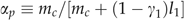 . Here, we present a forecast‐update model that allows us to develop closed‐form solutions for the CM's decision when the forecast update contains some new information about demand, but some demand uncertainty still remains. As we point out below, however, Zhang (2005) shows that this demand model provides closed‐form solutions that very closely approximate numerically computed solutions to the bivariate‐normal case.
Suppose demand D follows a uniform distribution, D∼U[μ−δ, μ+δ], where the parameters μ and δ are both known at LT
2. At LT
1, we assume that the width parameter δ is known, but the mean, μ, is a uniformly distributed random variable, with 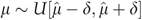 , where
  is the expected value of μ at time LT
1. In this context, μ is the information random variable. Let
is the expected value of μ at time LT
1. In this context, μ is the information random variable. Let  and
and  denote the lower and upper limits of μ, respectively. Given a choice of δ, we define
  . With this structure, the demand distribution at LT
1 is a symmetric triangular distribution with lower and upper limits given by
. With this structure, the demand distribution at LT
1 is a symmetric triangular distribution with lower and upper limits given by  . We call this the U–U demand model.
We note here that if the half‐width, δ, of the demand distribution at LT 2 does not equal the half‐width of the distribution on the mean parameter μ, then the convolved distribution at LT 1 is not triangular. For the case where these half‐widths are equal, the variance of demand at LT 2 is half the variance of demand at LT 1. 1 While this may seem restrictive, we note first that this is necessary in order to obtain closed‐form solutions and second, as we will see below, an interpolation technique can be used to effectively approximate cases where the quality of the forecast update varies.
4.2. CM Decisions with the U–U Demand Model
The development of the CM's cost function when the U–U forecast update is provided follows the same pattern as the general case from Section 3.2. The cost function here must be decomposed into several parts to account for the upper and the lower limits on the distributions of overall demand, the realized mean at LT 2 and the component 1 decision Q 1. Since the development is logically the same as the general case, but cumbersome due to multiple integration end‐point considerations, we include the details in Appendix A. The following proposition describes the optimal component 1 order quantities.
P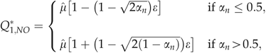
 .
.
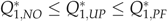
The fact that better forecast‐update information leads to a larger Q 1 * is best understood by the fact that when a forecast update will be provided, the CM commits only to component 1 at LT 1. This effectively reduces her overage risk exposure. So, it is the expectation of the update that causes the CM to increase her component 1 order. This is why it is important that the OEM provides (or does not provide) updates as policy rather than deciding at LT 2 whether or not it is in his interest to share the update.
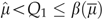
The condition  on the first expression in Equation (10) determines whether or not forecast updates are useful to the CM. For a given risk‐sharing agreement, the values of α are fixed. If
  , then the CM will order Q
1 as if she was not receiving an update. Furthermore, it can be easily verified that there is no possible realization of the forecast update that would benefit the CM; for these cost parameters, her desired choice of Q
2 will always be greater than Q
1
*.
, then the CM will order Q
1 as if she was not receiving an update. Furthermore, it can be easily verified that there is no possible realization of the forecast update that would benefit the CM; for these cost parameters, her desired choice of Q
2 will always be greater than Q
1
*.
Let  represent expected shortages for a fixed risk‐sharing agreement assuming the CM orders both components optimally. Using these definitions and the expressions developed above, we can establish the following proposition.
P .
.
While providing forecast updates reduces shortages for this U–U model, recall that this is not true in general (Observation 1). Here, however, choosing to provide forecast updates will result in fewer shortages for the OEM for any fixed risk‐sharing agreement. This does not necessarily mean that it is always in the best interest of the OEM to provide forecast updates. As we will see below, that will depend on the choices of γ 1, γ 2.
It is worth recalling here that when there is no risk‐sharing agreement, the OEM's cost consists only of shortages. As the following corollary indicates, for this no‐risk‐sharing situation, both the CM and OEM are better off when the forecast update is provided.
C
While the U–U model is restrictive in the sense that it permits only two versions of forecast‐update quality (where the variance is cut in half and where the update is perfect), it does permit the development of closed‐form expressions. Although a bivariate‐normal forecast‐update model would have the advantage of allowing a range of more or less informative forecast updates, its disadvantage is that closed‐form solutions appear to be available only for the two extreme cases. The UP solution in expression (10), however, can be used to approximate the optimal component 1 order quantity, Q 1 *, for a bivariate normal model with varying levels of forecast‐update quality. The method—details for which may be found in Zhang (2005)—is to use linear interpolation, with the solutions at the two end points of the bivariate normal case (i.e., the perfect and worthless forecast‐update cases) plus expression (10), jointly allowing a three‐point interpolation in a piecewise fashion. Zhang (2005) compares the U–U‐based, three‐point interpolation with a simple two‐point linear interpolation that uses only the end points from the bivariate normal case. The three‐point approach outperforms the two‐point interpolation as an approximation to the bivariate‐normal model solutions in all cases, typically by a substantial amount. Across 29,700 cases over a grid of parameter values, Zhang (2005) finds that the maximum percentage error and average percentage error in total cost, as compared with the total cost of numerically computed bivariate‐normal solutions, are 2.18% and 0.08%, respectively, for the three‐point interpolation; this compares with 11.75% and 0.84%, respectively, for the two‐point approach.
So far, we have focused our discussion on demand forecast updating and its effect on the CM's ordering behavior, and we have presented some results regarding the OEM's decisions relative to providing the forecast update and offsetting the overage risk to influence the CM's ordering behavior. The sub‐section that follows will explore this contract‐mediated coordination between the OEM and the CM across a large set of computational experiments. We use the closed‐form solutions of the U–U model to investigate the impact of risk sharing and forecast updating to the OEM, the CM, and the overall supply chain.
4.3. Computational Results for U–U Demand Model
Recall that Corollary 2, stated above for the U–U model, indicated that forecast updating is always Pareto‐improving for the OEM and CM when there is no risk‐sharing agreement. This, however, leaves open the question of what happens when risk sharing and forecast updating are implemented jointly. Adding component risk‐sharing may help to better align the incentives of the CM with the outcomes for the OEM and thereby generate additional cost savings for both. The general results presented in Section 3, however, also indicate that providing the forecast update could make things worse for the OEM. Thus, there are a number of issues regarding the extent of the forecast updating and risk‐sharing effects in isolation, and the nature and extent of their complementary effects, that are not addressed by the analytic results. In this section, we use a broad set of computational experiments to help us understand the various effects listed above and to help us address the issue of how much improvement the OEM or CM could expect and under what conditions those improvements are larger, smaller, or perhaps negligible. We discuss our findings in a series of computational observations, detailed below. First, we investigate the impact of forecast updating and risk sharing on OEM cost. Then, we examine the impact that the OEM's choices have on the CM and the overall supply chain.
Using the U–U model, our straightforward, closed‐form expressions for order quantities, expected shortages, expected overages, and expected costs allow us to compute results for a large set of experiments with only modest computing power and time. We consider a relatively finely spaced grid of the four cost parameters in our model: m
o
, m
c
∈{0.1, 0.2, …, 1.5} and l
1, l
2∈{0.1, 0.2, …, 0.9}, resulting in 18,225 experiments for each forecast‐updating and risk‐sharing scenario we consider. Moreover, the fact that CM and OEM cost functions are all easily computed in closed‐form for given values of γ
i
allows us to easily find the values that minimize C
oem
by searching over the (γ
1, γ
2) space. All cost results are stated in terms of percentage improvement over the base cost in question, which does not vary with different values of  and ɛ (since those parameters only scale the values of demand and order quantities, but do not change the relative cost outcomes).
Table 1 shows the mean, minimum, and maximum percentage difference in costs for the OEM between what we consider our base setting—no forecast update provided (NO) and no risk‐sharing contract (NC)—and the setting with both forecast updating (UP) and risk sharing through the DG contract. Starting from the base scenario (NO–NC), the OEM could offer only a forecast update (UP–NC), offer only to share component overage risk (NO–DG), or offer both (UP–DG). All comparisons in Table 1 are back to the NO–NC scenario.
NC, no contract; DG, dual‐gamma.
C
Recall that Observation 2 in Section 3.2 demonstrated that it is possible for forecast updating to increase OEM cost. Note, however, from Table 1 that the minimum reduction in OEM cost going from NO–NC to UP–NC is zero (no reduction, but also no increase). Moreover, across our set of 18,225 experiments, we found no cases in which C oem increased between the NO–DG and the UP–DG solutions (a comparison not shown in Table 1).
C
As noted above, there is little positive complementarity between providing forecast updates and sharing overage risk, on average. Figure 3 allows us to probe this issue further by examining this interaction on a case‐by‐case basis. The left panel in this figure plots the OEM percentage cost improvement due to risk‐sharing when forecast updates are provided (UP–DG improvement over UP–NC) vs. the OEM percentage cost improvement due to risk sharing when forecast updates are not provided (NO–DG improvement over NO–NC) for each of our 18,225 experiments. All points in the plots represent a single case, or combination of the cost parameters m o , m c , l 1, l 2. The right panel plots the OEM cost improvement due to providing forecast updates for risk‐sharing (UP–DG improvement over NO–DG) vs. no‐risk‐sharing (UP–NC improvement over NO–NC).
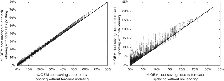
C
The results in Figure 3 and Table 1 raise an obvious question, namely, whether one could identify common cost characteristics that separate cases with high cost reduction for the OEM from those with low cost reduction. As one might suspect, the OEM tends to see the most benefit from risk sharing when the CM's margin, m c , is relatively small and the CM would otherwise tend to place smaller component orders to avoid relatively expensive overage costs. For example, across the cases where the decrease in C oem from NO–NC to NO–DG is at least 20% (which represent about 15% of the experiments), the average value of m c is slightly more than 0.2. On the other hand, cases where that comparison nets out to no change in C oem have an average m c of slightly more than 1.05. Not surprisingly, the comparative values of m o are higher in those cases where the OEM benefits most. (Comparative statistics on l i across these cases are uninteresting, spanning all values and averaging about 0.5.) The results are similar in comparing UP–NC with UP–DG cases.
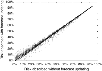
A related issue is whether the optimal amount of risk absorbed by the OEM is different between the NO and UP scenarios. Since γ
1 and γ
2 reflect the fraction of the component 1 and 2 overage losses, respectively, offset by the OEM, the percentage of the total component overage risk absorbed by the OEM is (γ
1
l
1+γ
2
l
2)/(l
1+l
2). Figure 4 shows a plot of the risk absorbed by the OEM without forecast updating (NO) and with forecast updating (UP). In the majority of our experiments (10,438 cases or 57.3%), the level of risk absorbed is the same with forecast updating (UP) and without (NO)—i.e., those cases that lie on the y=x line in Figure 4. In fact, roughly 84% of the cases lie near the line, where “near” is defined to be a difference in risk absorbed of no more than 1% in either direction. Furthermore, on average, the OEM's optimal level of risk sharing is roughly the same whether or not a forecast update is provided to the CM as a matter of policy (the average amount of risk absorption is 20.2% across the NO cases and 20.3% across the UP cases). Across the set of cases with no difference in the level of risk absorption, the average value of m
c
for these cases is  , with
  . By contrast, for the cases in which either less risk (27.0% of cases) or more risk (15.7% of cases) is absorbed when the forecast is provided, the relative values of margins flip:
  and
and  for the cases where less risk is absorbed under UP, and
  and
and  for the cases where more risk is absorbed under UP. Again, the difference in OEM and CM margins appears to dictate the nature of the outcome.
C
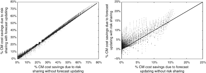
Now, we consider the impact of the OEM's forecast‐updating and risk‐sharing actions on the CM's cost outcomes. Table 2 shows CM cost results across all computational experiments, similar to Table 1 for the OEM. Figure 5 shows case‐by‐case plots of the percentage cost improvement for the CM that parallel those shown above for the OEM (Figure 3).
NC, no contract; DG, dual‐gamma.
C
In light of the results shown in Figure 4, the results in the left panel of Figure 5 are not surprising. That is, given that the OEM will absorb roughly the same amount of risk under the different forecast‐update settings, we might expect the CM's benefit to be roughly the same in these two settings. The right panel of Figure 5, however, begs further discussion. First, note that there are cases where the CM's cost increases due to forecast sharing. (Recall that the y‐axis here shows the change in cost from NO–DG to UP–DG. Note also that this is different from the comparisons with NO–NC reported in Table 2.) Details for this relatively small subset of the computational experiments are shown in Table 3 (about 3.5% of the total cases studied, and <0.5% if one restricts the subset to those cases where CM cost increases by 1% or more). The bottom portion of Table 3, which compares the level of risk absorbed by the OEM without forecast updating (left column of each pair) and with forecast updating (right column), explains what happens in these cases where the CM cost increases. As one can see from these comparisons, in the small number of cases (0.07% of experiments) where the CM cost increases by 2% or more, the OEM absorbs significantly less of the overall overage risk (45% vs. 52%) when it offers the forecast update in conjunction with the risk‐sharing contract. As we indicated earlier, the OEM's provision of a forecast update may indeed reduce the OEM‐optimal risk offset to the CM, and now we see that this reduction in overage offset can, in some cases (although not many, among our experiments), exceed the cost savings to the CM from forecast updating. As we consider less dramatic levels of cost increase for the CM, however, the situation begins to “regress to the mean” for the overall set of experiments, namely that the OEM absorbs roughly the same level of risk with and without the forecast update (recall our discussion of Figure 4).
CM, contract manufacturer; DG, dual‐gamma; OEM, original equipment manufacturer; NO, no forecast update; UP, forecast update.
C
After examining the impact of risk sharing and forecast updating to both the OEM and the CM, we turn our attention to the impact to the overall supply chain. Above, we observed that forecast updating and risk sharing, either in isolation or together, always reduce OEM cost and nearly always reduce CM cost. For each of our cases explored above, we compare the outcome under the OEM's choice with the supply‐chain‐optimal solution. (The supply chain optimal solution, labeled CP for centrally planned, is easily obtained by solving what we formulated as the CM's problem, but instead using the total supply chain shortage cost, m o +m c , and component overage costs, l 1, l 2. This can be done for both forecast‐update and no‐forecast‐update cases.) We define the contract efficiency of each forecast‐update, risk‐sharing solution to be the ratio of (1) the cost reduction achieved by that solution over the NO–NC case and (2) the cost reduction achieved by the centrally planned solution with forecast updating (UP–CP) over the NO–NC case. Table 4 shows the mean, minimum, and maximum contract efficiencies.
CP, centrally planned; NC, no contract; DG, dual‐gamma.
C
From the table, we see that the forecast‐updating policy under the risk‐sharing contract (UP–DG) captures over 61% of the first‐best reduction in supply chain cost, on average. Interestingly, this is nearly the same improvement over the no‐contract case as a centrally planned solution with no forecast updating (NO–CP). For completeness, we note that in <1% of the total experiments, the supply chain cost increased when a forecast was provided under OEM‐optimal risk sharing—i.e., comparing supply chain costs under NO–DG and UP–DG solutions—but never by >0.02%.
5. Conclusions
In this paper, we have examined how an OEM might use forecast‐update sharing and component overage risk sharing to effectively coordinate with a CM that produces a sub‐assembly of complementary components with different lead times. In Section 1, we presented several questions concerning the OEM's forecast‐updating and risk‐sharing decisions. To address these questions, we developed some general results as well as a specific U–U forecast‐update model that permitted further analytic results, and also performed extensive computational experimentation. Here, we reconsider the questions posed in Section 1 and summarize how our findings answer these questions.
(1) Under what conditions should the OEM provide a forecast update?
Consider the case when there are no risk‐sharing agreements in place. With no risk‐sharing agreement, updating the forecast tends to cause the CM to provide better product availability. We prove that this is true for our U–U demand model. (Additional runs using a bivariate normal demand model, although not the subject of this research, provided no countervailing cases.) We also, however, present a discrete‐demand example (where the convolved distribution at LT 1 is bimodal) where a forecast update can result in lower product availability (higher shortages). Thus, it is possible for forecast‐update sharing to hurt the OEM. So, absent a risk‐sharing agreement, should the OEM share forecast updates? The existence of a counter‐example makes the scientific answer “it depends.” The analytic result for the U–U model (and our additional computational experience with a parallel bivariate‐normal model) would seem to indicate that if the demand distribution at LT 1 is not bimodal, and no risk‐sharing agreement is in place, providing a forecast update is probably a good idea for the OEM.
(2) Under what conditions should the OEM offer to share component overage costs with the CM?
In general, sharing overage risk on components is an effective lever that an OEM can use to influence the CM's ordering behavior. We demonstrate analytically that sharing overage risk causes the CM to increase its purchase quantity of the longer‐lead‐time component. Our computational experiments suggest that under a specific forecast‐update setting, substantial cost reductions are attainable by using risk‐sharing agreements. Not surprisingly, cases where the CM has a cost incentive to order small quantities of components—cases with low CM margins—present the greatest opportunity for OEM cost improvement via risk‐sharing agreements.
(3) How do the decisions to provide a forecast update and share component overage costs interact?
First, recall that Figures 3 and 5 demonstrated that, on average across our computational experiments, there is only a slight interaction between forecastupdating and risk sharing in terms of their effects on OEM and CM costs. The cases in which risk sharing demonstrated some positive interaction with forecast updating for the OEM were those in which the cost savings were relatively low under forecast updating alone. For the CM, this slight positive interaction is even less pronounced, particularly in terms of risk sharing, which demonstrates much more widely dispersed effects on the CM cost savings from forecast updating. Moreover, while we show by a discrete‐demand example that it is possible for the OEM to be hurt by providing the forecast update under the DG contract, this never happened in our set of U–U computational experiments. It would be interesting, however, to consider future research that explores forecast‐updating–risk‐sharing interactions for less well‐behaved demand‐update distributions.
(4) How do the OEM's decisions affect the CM and the supply chain as a whole?
We show analytically that at the optimal level of risk sharing for the OEM, the CM's optimal order quantity is less than the OEM would prefer and also less than the optimal quantity for the overall supply chain. Thus, given that the OEM will act in his own best interest, the contract structures studied here will not optimize the overall supply chain. We identify contract parameters that will perfectly coordinate the supply chain if fixed side payments are permitted. In our computational experiments, however, the OEM's best option (provide forecast updates and use DG risk sharing) captured 61.3% of the potential total supply chain improvement. Moreover, our computational experiments suggest that forecast updating and risk sharing appear to be equally beneficial to the OEM when applied separately, and that their combined effect can result in significant cost improvements over a no‐updating, no‐risk‐sharing policy. Similarly, the potential cost savings of these policies for the CM can be substantial, and, although the effects of risk sharing on CM cost savings due to forecast updating display greater dispersion than they do in the OEM case, the relative impact of risk sharing and forecast updating on CM costs overall is, as it is for the OEM, about the same. Finally, among the set of choices modeled here, we observe that sharing the forecast update and using the DG contract was always best for the OEM, almost always best for the CM (96.5% of the time), and always best for the overall supply chain (save a small number of marginal cases).
Appendix A
P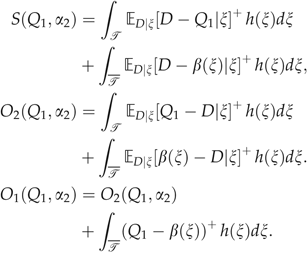
The partial derivatives of these objects with respect to Q
1 and α
2 are 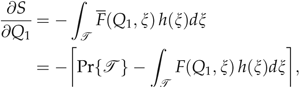
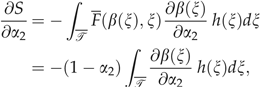
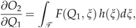
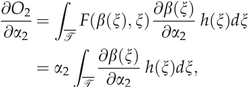
Recall β(ξ) is the inverse of a cdf and therefore must be non‐decreasing in α 2. It is immediate from the above expressions that shortages are non‐increasing in Q 1 and α 2, overages of component 2 are non‐decreasing in Q 1 and α 2, and component 1 overages are non‐decreasing in Q 1 and non‐increasing in α 2. □
P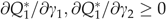 , we will use the derivatives of critical fractiles, α
2 and α
n
, with respect to γ
1 and γ
2
, we will use the derivatives of critical fractiles, α
2 and α
n
, with respect to γ
1 and γ
2
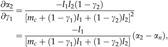

It is clear that expressions (A7) and (A8) are non‐positive (non‐negative), establishing the second part of the result: α 2 is non‐increasing (non‐decreasing) in γ 1 (γ 2).
In order to establish the first part of the result, we will use the derivative of CM cost (Equation [7]) with respect to Q
1. Using derivative expressions (A1), (A3) and (A5) from the proof of Proposition 1 above, we can write the derivative of CM cost with respect to Q
1 as follows: 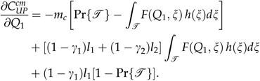
Assuming strictly non‐negative cost parameters m
c
, l
1, l
2, we have that the term inside brackets must equal zero at the CM's optimal Q
1
*. Rearranging, this gives 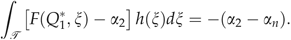
Differentiating both sides of the above equation with respect to γ
1 yields 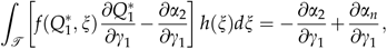

Similarly, the derivative of Q
1
* with respect to γ
2 is 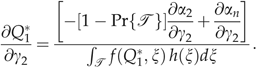
Using expressions (A8) and (A10), this can be re‐written as 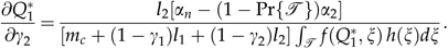
Rearranging the CM's first‐order optimality condition (A13), 
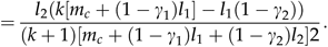
P on γ1, γ2. Note that any optimal γ
1, γ
2 for the OEM must satisfy the OEM's first‐order optimality conditions:
on γ1, γ2. Note that any optimal γ
1, γ
2 for the OEM must satisfy the OEM's first‐order optimality conditions: 
 denotes the partial derivative of
  w.r.t. Q
1 evaluated at Q
1=Q
1
*. Using derivative expressions (A1), (A3) and (A5) from the proof of Proposition 1 above, we can write the derivatives of the OEM's cost with respect to Q
1
* and α
2 as follows:
w.r.t. Q
1 evaluated at Q
1=Q
1
*. Using derivative expressions (A1), (A3) and (A5) from the proof of Proposition 1 above, we can write the derivatives of the OEM's cost with respect to Q
1
* and α
2 as follows: 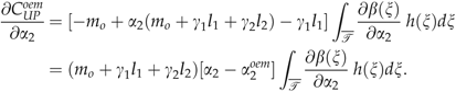
 and
and  .
.
To establish the result, we must show that  at a point (γ
1
*, γ
2
*) that satisfies the OEM first‐order conditions. We will proceed by supposing that there exists a case where this is not true and deriving a contradiction. Specifically, we will show that if
at a point (γ
1
*, γ
2
*) that satisfies the OEM first‐order conditions. We will proceed by supposing that there exists a case where this is not true and deriving a contradiction. Specifically, we will show that if  at a point (γ
1
*, γ
2
*) that satisfies the OEM's first‐order conditions, then there exists a direction in which the OEM could move away from (γ
1
*, γ
2
*) and reduce his cost, contradicting the fact that (γ
1
*, γ
2
*) satisfies the first‐order conditions.
at a point (γ
1
*, γ
2
*) that satisfies the OEM's first‐order conditions, then there exists a direction in which the OEM could move away from (γ
1
*, γ
2
*) and reduce his cost, contradicting the fact that (γ
1
*, γ
2
*) satisfies the first‐order conditions.
Suppose the OEM moves (γ
1, γ
2) simultaneously in the direction [1, k]. The derivative of OEM cost with respect to γ
1, γ
2 moving in this direction is 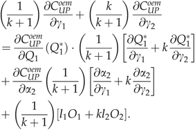
First, we consider how α
2 changes when γ
1, γ
2 move in this direction: 
 , the term inside the parentheses in the numerator of (A26) is zero; as we move γ
1, γ
2 in this direction, α
2 is unchanged. With this choice of k, therefore, the directional derivative for OEM's total cost is determined only by the change in cost due to changes in Q
1
*. So, we can drop the second term in (A24) above. Substituting expressions (A15) and (A16) gives:
, the term inside the parentheses in the numerator of (A26) is zero; as we move γ
1, γ
2 in this direction, α
2 is unchanged. With this choice of k, therefore, the directional derivative for OEM's total cost is determined only by the change in cost due to changes in Q
1
*. So, we can drop the second term in (A24) above. Substituting expressions (A15) and (A16) gives: 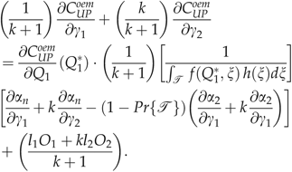
By our choice of k, 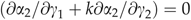 , and, from Proposition 1,
 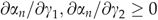 . Furthermore, by supposition,
 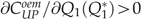 . This means that this directional derivative is strictly positive, contradicting the optimality of γ
1
* and γ
2
*. So, at (γ
1
*, γ
2
*),
. This means that this directional derivative is strictly positive, contradicting the optimality of γ
1
* and γ
2
*. So, at (γ
1
*, γ
2
*), 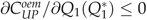 .
.
To establish the second part of the proposition, note that the total supply chain cost is equal to the sum of the CM's and OEM's costs; thus, 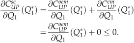
As a final note, recall that since the CM's cost function is convex, Q 1 * is unique for any given values of (γ 1, γ 2). We have not established that there is a unique (γ 1 *, γ 2 *) pair for the OEM. Rather, this proof establishes that at any (γ 1, γ 2) that satisfies the first‐order conditions (which would include an optimal solution) the OEM and the supply chain would benefit from an increase in Q 1 from the CM's optimal choice Q 1 *.
P
To establish our claim, we must show that, with values of  , the CM will make decisions that also optimize the supply chain. With these values, the CM's cost function is
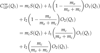
Multiplying the CM's cost function by the constant  will clearly not change her optimal component ordering choices,
The right hand side of Equation (A30) is the same as the cost for the overall supply chain, establishing that, with γ 1, γ 2 as specified, the CM will choose order quantities that minimize supply chain cost.
CM Cost Function with U‐–U Forecast‐Update Model
For this model, the demand‐related information that is obtained between LT
1 and LT
2 is the realization of the mean, μ. Using the inverse function of the uniform distribution, we can calculate the component 2 quantity that the CM would want to buy,  . As before, this may be constrained by the choice of Q
1. We also define
. As before, this may be constrained by the choice of Q
1. We also define 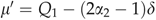 to be the value of μ at which Q
1=β(μ). Using the set notation from the previous section, T would be the set of realizations of μ≥μ′, i.e., where the CM will order components in equal quantities. Given Q
1, we can formulate the CM's cost function by conditioning on μ.
to be the value of μ at which Q
1=β(μ). Using the set notation from the previous section, T would be the set of realizations of μ≥μ′, i.e., where the CM will order components in equal quantities. Given Q
1, we can formulate the CM's cost function by conditioning on μ.
If If If If
 , the CM will order Q2 equal to Q1. Her cost expression in this case is the same as that when no update is provided.
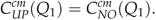
 , the CM's cost expression is
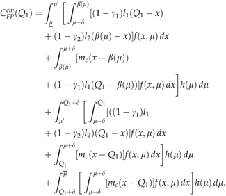
 , the CM's cost expression is
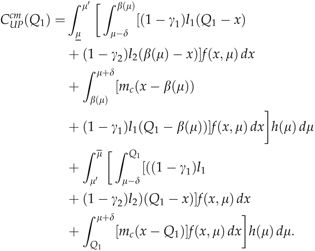
 , the CM will always choose Q
2=β(μ). Her cost expression is
, the CM will always choose Q
2=β(μ). Her cost expression is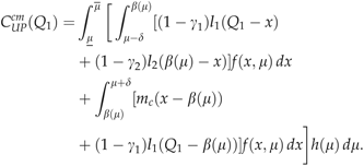
P
Both results for the U‐–U model follow from straightforward algebra. Proofs are available from the authors.
Footnotes
Acknowledgments
The authors would like to thank the anonymous referees and Senior Editor for their extensive and very helpful efforts in improving the model and analysis presented in this paper. We would also like to thank Brian Eck and Clayton Berlinghoff of IBM Corporation and Burt Proctor of Solectron Corporation for their advice and counsel in accurately representing OEM–CM interactions in practice. We also acknowledge the helpful comments and suggestions of the participants in research seminars at Olin Business School at Washington University, the Johnson School at Cornell University, the Department of Industrial & Systems Engineering at Lehigh University, and North Carolina State University's Graduate Program in Operations Research and College of Textiles. This work was supported in part by funding from IBM Corporation and from the Center for Supply Chain Research in the Smeal College of Business at Pennsylvania State University.
1Variances at LT 1 and LT 2 are 2δ/3 and δ/3 respectively.