
Abstract
This paper examines the optimal product portfolio positioning for a monopolist firm in a market where consumers exhibit vertical differentiation for product performance and horizontal differentiation for product feature. Our key results are as follows: (i) Variable costs drive vertical differentiation. In the presence of significant volume‐dependent manufacturing costs, the optimal portfolio contains a mix of vertically and horizontally differentiated products and an increase in the variable cost makes adding vertically differentiated products relatively more profitable; if fixed volume‐independent design costs dominate, the portfolio exhibits solely horizontal differentiation. (ii) Horizontal differentiation is the main profit lever, and vertical differentiation brings only a marginal benefit; this is true even when most of the consumers exhibit low willingness to pay for performance, which is often used as an excuse to offer low‐end products. (iii) There are more low‐quality products than high‐quality ones, and market coverage increases when the willingness to pay for performance increases. In summary, the model shows how portfolio composition decisions depend on the product cost structure and the consumer preferences.
Keywords
1. Introduction
Product designs are usually defined by multiple attributes. We group these attributes into two main categories: the horizontal and the vertical differentiation dimensions. In product design terminology, the horizontal differentiation dimension represents the “feature” choices of product design, whereas the vertical dimension captures the product performance (also referred to as “quality,” a well‐established driver of consumer willingness‐to‐pay, Mussa and Rosen (1978). Throughout the paper, we use the terms “performance quality” and “quality” interchangeably). For example, in MP3 players, a vertical quality dimension is memory size (all customers agree that larger memory size makes the player a more attractive purchasing option), and horizontal feature dimensions are color, shape, and other “taste” design attributes (customers have different preference on this dimension; they disagree which color or shape is the best). This paper examines the optimal portfolio for a consumer market with both vertically and horizontally differentiated preferences.
Market structure models that combine horizontal and vertical differentiation in consumer preferences are essentially intractable (Heeb 2002). In order to present analytical results, past literature has either intentionally reduced the mathematical degrees of freedom by examining uni‐dimensional markets (Lancaster 1998) or made a “market coverage” assumption (all customers must buy one and only one product) (Economides 1993, Neven and Thisse 1987). Past studies have alternatively imposed a consumer wealth constraint to force separate demographic‐like segments (e.g., different income groups) (Weber 2008), pre‐segmented the market into fixed segments (“high quality” and “low quality” consumers, “blue” and “red” customers, “primary” and “green” consumers; Adner and Zemsky 2005, Atasu et al. 2008, Kim and Chhajed 2000, Krishnan and Gupta 2001), or, finally, restricted the types of products and focused on “development intensive products” (DIPs) dominated by fixed costs, such as software, movies, or other information products (Krishnan and Zhu 2006). We do not restrict the product cost structure or the market behavior in any of the aforementioned ways, and we examine the decision of placing any arbitrary number of products in the market. In order to concentrate on the cannibalization among products, we do not consider the products of other firms (competition), but rather focus on a monopoly. As this type of model is mathematically intractable, only part of the results can be obtained analytically; we use numerical studies to generalize our results. Our intention is to study the optimal product portfolio composition addressing endogenously formed customer segments, and to indicate the number of products the market can beneficially support.
We find that the variable cost of quality drives vertical differentiation and that horizontal differentiation offers a larger profitability lever than vertical differentiation. In other words, as variable quality costs increase relative to fixed quality costs, offering another product line with a different quality becomes an attractive option. Still, growing the product portfolio should focus first on the potential of differentiated features (but the same performance quality), and only then exploit consumers along the quality dimension. Subsequently, market coverage increases when willingness to pay increases. Interestingly, the optimal portfolio should contain more low‐quality products than high‐quality ones. The results hold in a surprisingly wide range of circumstances, and have significant managerial implications.
We establish our results as follows. In Section 2 we review past literature, and in Section 3 we present the model structure and premises. The simplest case of one product is analyzed in Section 4. Section 5 studies the optimal portfolio for DIPs. In Section 6, we analytically derive the key results (adding vertically differentiated products adds little profit, but is profitable after all in the presence of high variable cost) for a special case. Section 7 provides numerical evidence that the results of Section 6 hold also for the general cost structure, and that the results hold true even when customers are concentrated at the low‐quality end of the market. We conclude and discuss our overall framework in Section 8.
2. Literature Review
The theory of product differentiation begins with Hotelling's (1929) horizontal differentiation model. In his model, consumer utility decreases with the price and the distance between the ideal feature desired by the consumer and the product feature offered. In such a market, two competing profit‐maximizing firms choose, in equilibrium, the same price and feature, and they have the same market share and profit. Tirole (1988) shows that when transportation costs are linear, two competing firms seek maximum differentiation in location. Doraszelski and Draganska (2006) investigate the joint effect of competition, cost structure and feature fit. Green and Krieger (1985) present an algorithm to position multiple products in the absence of competition. Hansen et al. (1998) present an algorithm to position a product in multi‐attribute space, where each consumer has an ideal point and chooses the product with the smallest Euclidean distance from this point.
In vertical differentiation, consumers have different valuations for the performance quality of the same product (Mussa and Rosen 1978). Consumer utility increases both in performance quality and the valuation of performance quality. Vandenbosch and Weinberg (1995) study two costless quality dimensions, and Krishnan and Zhu (2006) study two costly quality dimensions. Tirole (1988) shows that, if all consumers purchase one of the two products offered, competing firms will seek maximum differentiation in quality, one choosing maximum quality and the other choosing minimum quality. If not all consumers buy, the firms will still seek differentiation, but not maximum differentiation (Moorthy 1988). Moorthy and Png (1992) study the sequential introduction of new products into a vertically differentiated market space. Cremer and Thisse (1991) show that when there is only variable cost, horizontal differentiation is a special case of vertical differentiation. In Wauthy (1996), the optimal product line highly depends on the distribution of consumer preferences with respect to their performance quality valuation. A distribution with higher dispersion results in a partially covered market space. Chen et al. (2008) analyzed multi‐function products, which may be viewed as vertically differentiated from single‐function products.
Some studies have combined both types of differentiation. Neven and Thisse (1987) model competing firms in a two‐dimensional market space. To assure tractability, they assume that all consumers derive positive utility from buying one of the products on the market, the so‐called “market coverage assumption.” Then, the equilibrium depends on the relative magnitude of these two dimensions, and both firms choose maximum differentiation in the relatively wide dimension and minimum differentiation in the “narrow” dimension. Heeb (2002) shows that relaxing this assumption does change the final equilibrium and makes numerical analysis necessary. Ferreira and Thisse (1995) use a “transportation rate” to replace the fixed weight of the difference between the ideal feature and the product's actual feature in the consumers' utility function. We do not assume market coverage, since we examine which part of the market space is covered.
Certain research papers focus on products with only per‐unit manufacturing cost (no volume‐independent design cost). Moorthy (1984) uses product cannibalization to provide an alternative explanation for the aggregation of segments, as opposed to the usual economies of scale argument. Chambers et al. (2007) show that slight change in variable cost can result in very different equilibria, which offers an explanation of the outcome diversity we observe in practice.
In contrast, another stream of research assumes negligible per‐unit manufacturing costs and significant volume‐independent design costs (such products are called DIPs; see Krishnan and Zhu 2006). When consumers are characterized by two ordered quality preferences, degrading a high‐end product to obtain a low‐end product is sub‐optimal. Krishnan and Gupta (2001) consider both a design cost and a unit production cost, for a one‐dimensional vertical market, to identify when a platform design is justified. They conclude that platforms are not appropriate for extreme market diversity or high economies of scale. The model in this paper considers products with both volume‐independent design costs and volume‐dependent manufacturing costs, in a two‐dimensional market space. We demonstrate that unit production cost drives quality differentiation. We also identify the potential strategies to design product families, i.e., whether and when firms should introduce horizontally or vertically different product variants.
Table 1 summarizes the positioning of the papers discussed above, according to the types of costs considered and the assumed market structure.
3. Model Setup
In this section, we define the major concepts of our model: the product characteristics, the market space structures, and the firm's objective function.
Product: We posit that a product's design attributes can be represented through two distinct dimensions: the design features f, and the performance quality q. For example, in a desktop computer, design features might be the color or design of the tower box, the mouse used, or the arrangement of the keyboard. The features' influence on the costs is negligible; they represent design adjustments that respond to varying customer tastes and do not make the product overall “better” or “worse.” The performance quality might be the RAM or ROM memory, or the CPU speed. Quality decisions have an important impact on design and production costs.
The total cost of each product comprises two major components: the fixed investment during design and manufacturing system development, and the per‐unit variable manufacturing cost. Both types of costs are quadratic functions of quality and independent of the feature. Therefore, designing a product of quality q and producing k units of it costs C(q, f)=ksq 2+Sq 2. Similarly, designing another product with a different feature f′ but same performance quality costs another C(q, f′)=ksq 2+Sq 2. The quantity of the design feature f does not appear in the formula and has no impact on cost, but it is essential for the completeness of every product. This is to say that the design feature bears some cost—the various design variants of the feature all cost the same, while not having the feature at all implies one less product. Finally, s and S are two unrelated fixed parameters to represent the rate of increase of the marginal design and production cost in quality, respectively.
We do not consider economies of scope, or the possibility that s and S may decrease with the number of products, because this would complicate the analysis without qualitatively changing key insights (if introducing additional products becomes cheaper, the optimal number of products increases). The quadratic structure of costs is an approximation of a general convex cost function widely observed in practice, and it has been commonly employed in the research literature (Neven and Thisse 1987). If costs increase linearly in quality, the model is not significantly more tractable and does not yield different insights. The monopolist must decide at which unit price p to sell the product. In summary, the vector (p, q, f ) defines a product.
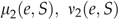
Market Space: The market space has two dimensions, which reflect consumer preferences about the product attributes. Customers are heterogeneous in their feature tastes and in their valuation of quality. The horizontal dimension captures the ideal feature of the product desired by each consumer. Each consumer has some ideal feature a∈[0,1] and suffers a quadratic utility loss if the product deviates from the ideal feature. The feature ranges from 0 to 1, for example, as color ranges from dark to light. This is just a way to denote different choices on this dimension; it does not imply any rank‐ordered preferences. For example, a product with a feature value of 0.7 does not have more features or superior performance than a product with a feature value of 0.5, only a lighter color.
The vertical dimension represents the consumers' valuation of product performance quality, denoted by b∈[0, 1]. All consumers appreciate more quality: a product with a quality value of 0.7 does have higher quality than a product with a quality value of 0.5. However, consumers are heterogeneous in the value b that they place on additional quality.
In summary, we denote the consumer market space by the set  . The different consumer valuations of the product features and performances are distributed according to a known joint probability distribution. We assume the density function m(a, b) over the market space M to be uniform: m(a, b)=1, ∀a∈[0, 1], ∀b∈[0, 1]. In Section 7, we relax this assumption to examine how the concentration of customers in a region of the market space influences the optimal portfolio.
The consumer with preference a in the horizontal dimension and valuation b along the vertical dimension enjoys utility  from buying the product (p, q, f). The first part, bq, captures the ordered nature of consumer preferences with respect to the performance quality. The second term, (a−f)2, represents the utility loss due to the deviation of the product feature from her/his ideal preference. The scalar e is the marginal utility loss from a unit of deviation. The marginal utility loss is common across all consumers and products. This assumption allows us to isolate the cost effects on product positioning. Should the customers at the high end become choosier (e increases with b), all demand curves would have sharper slopes; but this would not qualitatively alter the key results.
Objective function: A monopolistic firm maximizes profit with respect to the size of the product portfolio, and the quality, feature, and price of each product within the portfolio. We can write the objective function as follows: 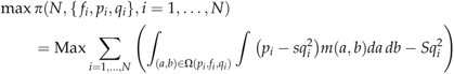
 is the subset of all consumers (a, b) that derive the highest non‐negative utility from product i.
4. Optimal Positioning of One Product
We start with the simplest case of one product in the market space, which sets the stage for the more‐complex setting of multiple products. Since the distribution of customer valuations is uniform, the product demand equals the market space area where consumers enjoy non‐negative utility. Define the curve  as the indifference curve, i.e., all consumers who are indifferent to purchasing the product (p, q, f). By solving
 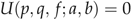 , we have
  . The consumers with profiles (a, b) above L, i.e.,
  , purchase the product.
Figure 1 shows the potential ways in which the product demand area A may fit into the market space M. A is defined by the curve L. There are three distinct possibilities of how L intersects the side boundaries of M: (i) they do not intersect; (ii) they intersect on both sides; and (iii) they intersect on only one side. Define  , and
, and  . Then, the three cases are described as (i)
  and
and  , (ii)
  and
and  and (iii)
  and
and  .
.
Case 3 in Figure 1 cannot be an optimal product positioning: if we shift the grey area A along the horizontal axis, while keeping price and quality constant, the shaded area inside the market space, or demand, increases without further cost increase until we reach Case 1 or Case 2.
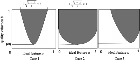
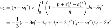
The profit functions in Case 1 and Case 2 are: 
Now we characterize the optimal positioning of the single product.
L (proof in
Appendix A
).
(proof in
Appendix A
).
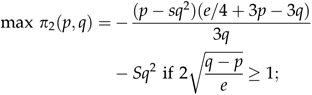
By Lemma 1, we can substitute  into the profit function (2) and then optimize with respect to price and quality. The optimization problem becomes:
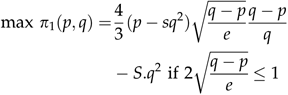
 .
.
It is straightforward to show that the derivatives of the function to the right and left of the boundary  are the same. Thus, the profit function is differentiable. The feasible regions are defined by the two boundaries p=0 and q=p. The profit approaches 0 as the variables approach these boundaries. Therefore, only an interior solution of (4) can provide a positive profit. When we solve the first‐order conditions (FOCs) of
 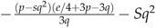 , we obtain at most four real solutions, regardless of whether the solutions fall into the feasible region
  . The FOCs of
  lead to at most six real solutions. Thus, for any given value of the parameters e, s, and S, we can determine the global optimum. However, we are unable to determine the parameter range under which a certain solution is the global optimum, because the 10 solutions have complex functional forms. We can characterize the optimal positioning of the single product for two special cost structures: when only the fixed cost or only the variable cost is present.
When the volume‐independent fixed cost is much greater than the production cost, such as for movies and software, we assume that the total cost equals the fixed cost, or s=0. We adopt the terminology of DIPs (Krishnan and Zhu 2006).
L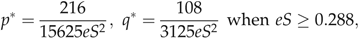
 when
when
 (the exact forms of
 are provided in the proof in the
Appendix A).
are provided in the proof in the
Appendix A).
Another special case is when the volume‐independent fixed cost is much smaller than the production cost; we assume that the total cost equals the variable manufacturing cost (Moorthy 1988), a case for trivial design changes. We label such products production intensive products.
L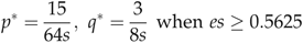
5. Optimal Positioning of N DIPs
Given the complexity of the single product case, we focus on the intuition we can build through boundary cases. We start with the special case of DIPs (Krishnan and Zhu 2006). The results for DIPs are obtained in several steps. First, we obtain the optimal price and quality, assuming that all products have the same price and quality. Then, we check the impact of a local deviation from this product portfolio on profit. Finally, we provide numerical evidence that this portfolio provides the global optimum for DIPs.
5.1. Symmetric Products
We now determine the optimal positioning of N products, assuming that N is fixed and that all products have the same price and quality.
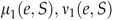
P
 is a
is a
 is a stationary point when es/N<ξ
h
. It is a
is a stationary point when es/N<ξ
h
. It is a
 are provided in proof in
Appendix A).
are provided in proof in
Appendix A).
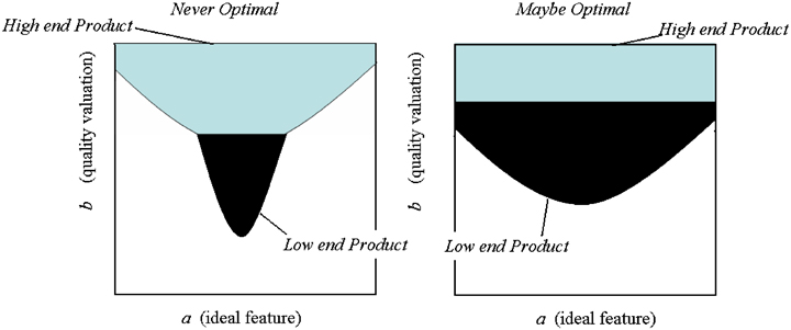
P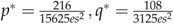 (as described in Lemma 2), and none of the products intersect one another or the side boundaries of the market space (see left‐hand picture in Figure 2), then this portfolio composition is optimal. It is indeed achievable to position N products in the market space without intersection when
 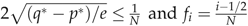 .
.

By substituting the optimal price and quality values into this constraint, we obtain the condition 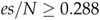 =ξ
h
. When es/N<ξ
h
, the products cannibalize one another (as shown in right‐hand picture of Figure 2). The number of potential configurations for the borders between neighboring products can become immense. It is this complexity that renders the analytical estimation of the global optimum impossible (Heeb 2002). Since all products have identical design costs and feature deviation losses, it seems a natural starting point to conjecture that they should be arranged symmetrically. Therefore, let all products have the same price and quality, and divide the horizontal (product feature axis) into N identical intervals, when each product feature takes the value
=ξ
h
. When es/N<ξ
h
, the products cannibalize one another (as shown in right‐hand picture of Figure 2). The number of potential configurations for the borders between neighboring products can become immense. It is this complexity that renders the analytical estimation of the global optimum impossible (Heeb 2002). Since all products have identical design costs and feature deviation losses, it seems a natural starting point to conjecture that they should be arranged symmetrically. Therefore, let all products have the same price and quality, and divide the horizontal (product feature axis) into N identical intervals, when each product feature takes the value  (see right‐hand picture in Figure 2a).
The profit function (1) becomes 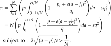
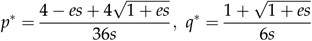
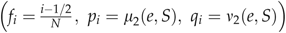
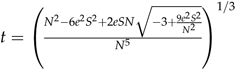
Observe that (9) is very similar to (3), except that the range of a is [0, 1/N] and f=1/2N. After some algebra, the optimal solution to (9) is 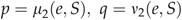 , the solution of the following set of polynomials with the greatest p value:
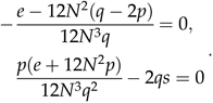
We denote this solution as  , which is identical for all products (i=1, 2, …, N).
When price and feature deviate from the portfolio proposed in Proposition 1 (ii), the boundary between two products is a vertical line (see left panel of Figure 2b):  (we obtain the border by solving
  while
while  ).
).
When the quality of a product deviates from the others, the boundary (see right panel of Figure 2b) 
 while
while  ). Therefore, a local deviation may result in a different functional form, depending on the direction of the change. We cannot write down a continuous profit functional form that we can derive. In addition, we cannot obtain all the second‐order derivatives (including cross derivatives), in order to calculate the Hessian needed to check local optimality. This is the reason why this model is analytically intractable: it is impossible to write down a common profit function at the neighborhood of a given point.
The symmetric portfolio proposed is a stationary point since the FOCs (necessary conditions for local optimality) are satisfied. We can check the profit change when the deviation of one variable happens on the axis. Assume that we change the price or feature of any product by δ: the profit change is negative. Assume that we change the performance quality of any product by δ. Denote the profit change as  . (
. ( contains more than 20 terms. It can be obtained from the authors upon request.) We approximate f(δ) at δ=0 through a Taylor's series expansion. Since
  , the local optimality is determined by f
(4)(0). We can show that f
(4)(0)>0 when es/N<ξ
l
. Therefore,
, the local optimality is determined by f
(4)(0). We can show that f
(4)(0)>0 when es/N<ξ
l
. Therefore,  and our conjectured product portfolio is a saddle point since the profit decreases with price deviation but increases with quality deviation. For ξ
l
≤es/N≤ξ
h
, f
(4)(0)<0 and quality deviation is non‐profitable. The intuitive explanation for the saddle point is as follows: when N, the number of products, surpasses a certain threshold, there are too many products in the market space and it becomes profitable to reduce their number. Our model has a fixed cost of introducing products, so the optimal number of products cannot go to infinity. Under these conditions, the symmetric portfolio becomes a local saddle point; reducing the price and quality of any product will increase profit. When the firm reduces the number of products again below that threshold, it again becomes unprofitable to decrease quality.
and our conjectured product portfolio is a saddle point since the profit decreases with price deviation but increases with quality deviation. For ξ
l
≤es/N≤ξ
h
, f
(4)(0)<0 and quality deviation is non‐profitable. The intuitive explanation for the saddle point is as follows: when N, the number of products, surpasses a certain threshold, there are too many products in the market space and it becomes profitable to reduce their number. Our model has a fixed cost of introducing products, so the optimal number of products cannot go to infinity. Under these conditions, the symmetric portfolio becomes a local saddle point; reducing the price and quality of any product will increase profit. When the firm reduces the number of products again below that threshold, it again becomes unprofitable to decrease quality.
Proposition 1 states that the symmetric product portfolio may be locally optimal. Previous work has observed that a uniform market space and the same cost structure across products lead to products with the same price and quality, but only by using the market coverage assumption (Economides 1993, Neven and Thisse 1987). Our analysis shows that the symmetric product portfolio is robust even without this assumption. When the market coverage assumption is violated, the classic result of maximum vertical differentiation in a duopoly no longer holds (Heeb 2002). Therefore, it is valuable to test whether the result concerning symmetric portfolio holds without this assumption.
Proposition 1 identifies a potentially optimal product portfolio of DIPs that uses only horizontal differentiation, without any vertical differentiation. Is this more generally true? We prove that a DIP product portfolio containing pure vertical differentiation is not optimal. We define pure vertical differentiation as designing products that have different qualities but are identical in their features.
P
Observe that the proof is based solely on revenues, independent of the details of the design cost structure. Therefore, even if the low‐quality product has a design cost advantage, pure vertical differentiation remains a non‐optimal strategic choice.
5.2. Numerical Studies
We have shown that, for a given number of products, pure horizontal differentiation (same qualities and price, different features) may be a local optimum, and that pure vertical differentiation (same feature) cannot be the optimal positioning for DIPs. This suggests an optimal portfolio composition. Still, we need to prove that there cannot be a global optimum in which products differ in price and quality. An analytical proof is out of reach due to the complexity of the model (three products have already hundreds of border scenarios). The closed form profit function cannot be written down. Therefore, we turn to numerical analysis. Our experiment design is characterized by two challenges: (i) the approximation of a “continuous” market space; and (ii) the performance of a significant number of numerical cases that guarantee the generality of our results. With respect to (i), we divide the market space into a 1000 × 1000 grid, with the grid accuracy being limited only by computation time. Then, for each product portfolio composition, we count the grid points that have positive utility to approximate demand.
We address concern (ii) as follows: for any deviation loss (e) and marginal quality cost (S), we calculate the profit for any size of a product portfolio that satisfies the conditions of Proposition 1. Then, we enter any initial value of price, quality, and feature for a fixed number of products N into a numerical search of the optimum using the Nelder–Mead algorithm (Nelder and Mead 1965). This search algorithm returns one local maximum as a result. If all search results we obtain from many starting values and many parameter constellations correspond to Proposition 1, the numerical study provides evidence that a symmetric portfolio is the global maximum.
We have performed two studies in the case of two and three products, due to computational limits. Study I has a large number of parameter values (100 (e, S) combinations; see Table 2) spread in the entire parameter space and relatively few starting values, whereas Study II has fewer parameter values but chosen in “sensible areas” and more starting values, and all starting values are chosen to represent most likely local optima (e.g., more lower‐quality products than higher‐quality products).
The curves in Figure 3 separate the parameter space (e, S) into regions where product portfolios of size 1, 2, or 3 are optimal. The black dots illustrate the chosen (e, S) combinations. We chose (e, S) combinations to make sure all regions are sufficiently represented. For each of these 100 (e, S) combinations, we chose four starting values to represent most likely local optima (therefore, a total of 400 experiments were performed). Table 1 summarizes the starting value choices. Q, the upper bound of quality, is a number slightly higher than the optimal quality of the one product case. Any initial value of quality provides an upper bound for the price since the price‐to‐quality ratio must be inferior to 1 by definition. We chose the initial values so that all possible price, quality, and feature combinations were sufficiently represented.
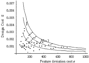
In Study II, to further validate our conjectures, we chose another 12 (e, S) combinations, as summarized in Table 3a, and 292 initial starting values for each (e, S) combination, as summarized in Table 3b (a total of 3504 experiments were performed). The (e, S) combinations are chosen near the borderlines where N products generate the same profit as N+1 products since these are the regions most sensitive to parameter change (see Figure 3).
In both studies, for any parameter set, the local optima of symmetric portfolio conjectured in Proposition 1 are indeed local optima, and they provide the maximum profit, with an error range around 1/1000. The error decreases as we use a finer grid. This provides evidence that Proposition 1 characterizes a globally optimal solution, at least for N=2 and N=3. For a larger number of products, the same algorithm can be used to confirm our conjecture.
5.3. Choosing the Optimal Number of Products, N *
The numerical results of Section 5.2 provide strong evidence for the global nature of the conjectured optimal portfolio composition, and allow us to perform a comparative static analysis on the optimal size of the product portfolio. Figure 4 depicts the optimal profit as a function of the feature deviation costs and the number of products for a fixed value of the marginal design cost, S=0.003. The dotted curves mark the profit‐maximizing frontier assuming overlapping products, whereas the solid ones mark the respective frontier for non‐overlapping products.
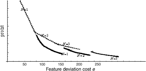
Not surprisingly, as feature deviation costs increase, the portfolio profit and the performance quality decrease, whereas the optimal size, N, increases. In addition, the overlapping frontier is consistently above the non‐overlapping one. In other words, it is better for all feature values to be served, despite the fact that they may cannibalize one another. In a portfolio, market coverage increases with willingness to pay.
Figure 4 indicates that a portfolio with cannibalization among its products dominates a portfolio without any cannibalization when the design cost parameter takes value S=0.003. This result holds true for any S, as the following argument shows. The profit function of the portfolio with cannibalization reads as 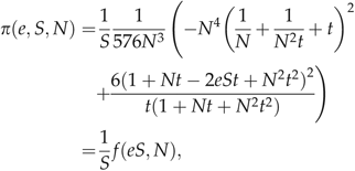
 Setting the derivative with respect to N to 0, the solution contains only the term eS. Hence, eS determines the optimal portfolio size. The profit function of the portfolio without cannibalization reads as
 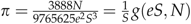 . When S takes another value, say S2, we transform the horizontal axis into
  . If
. If 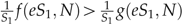 , then
 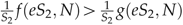 .
.
Figure 5 summarizes the optimal portfolio size, N, for each value of feature deviation cost, e. The optimal number of products increases as a step function, whereas the interval's length, within which a certain N is optimal, decreases in e. Figures 4 and 5 show that as e or S increases, each product optimally covers a smaller area and there are more products in the optimal portfolio.
6. Product Layers Without Fixed Cost
So far, we have focused on DIPs. The model suggests that the optimal portfolio of DIPs should use horizontal differentiation only, without vertical differentiation. This result is interesting but does not carry over to the general case. In this section, we introduce the key results of our model, that the presence of variable costs makes vertical differentiation possible. However, expanding the product portfolio along the vertical dimension offers a relatively smaller value, compared with adding horizontally differentiated products. We start the analysis with the opposite extreme case without fixed cost (S=0), where we can characterize the optimal portfolio in closed form. This special case begins building intuition as to why vertical layers do not add much profit. Section 7 analyzes the general case.
L
P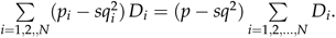 .
.
This function increases monotonically in the number of products as long as the margins are positive. As N↑∞, demand approaches (1−p/q). The horizontal dimension is no longer relevant, and the model becomes a one‐dimensional model (Moorthy 1988).
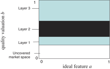
Figure 6 graphically illustrates the result one would intuitively expect. For any positive feature deviation cost e, it is optimal to add more horizontal products when there is no fixed cost. We define a “layer” of products as those with the same number of products directly (same feature) above and below them.
L
P
L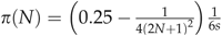 . The total profit increases monotonically by adding more layers of infinitely many products with identical price and quality within a layer.
P
For notational convenience, define two extreme (non‐existing) groups by  . Based on our definitions, the profit function becomes
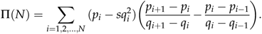
After some algebra, we can show that 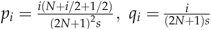 solves the FOCs of the profit function. We have shown for up to N=6 that this solution offers a higher profit than all other solutions of the FOCs and is, therefore, the optimal solution. We have been able to verify optimality up to N=6 and can repeat this verification for any specific higher value of N (we have not been able to prove, in general, for all N that this is the optimal solution). We substitute this solution into (11) and write the profit function as
  . It is easy to verify that the total profit increases with the number of products, and reaches a finite upper bound
  , as the number of layers approaches infinity. As layer 1 lies at the bottom of the portfolio, with the lowest price and quality,
  indicates the lower boundary of market coverage.
With Lemma 6, we can easily substitute the number N into the formula and obtain the profit for any layer. Based on our calculation, the maximum profit is 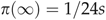 , when the number of layers is infinite. The first few layers of products capture the majority of the total potential profit. Specifically, the first two layers capture >95% of the maximum profit. For one layer, market coverage is 1/3, and as the number of the layers N approaches infinity, it approaches 1/2. Thus, total market coverage increases as the number of product layers grows, but the increase has decreasing returns.
7. Some Properties of the General Case
In Section 5, we argue that the optimal portfolio exhibits horizontal differentiation only when only fixed costs are present. In Section 6, we observe a combination of horizontal and vertical differentiation when only variable costs are present. In both special cases, we have “layers” of symmetric products with identical price and quality, and the same distances among features within each layer. Thus, it comes natural to conjecture that with a general cost structure, the optimal portfolio should also contain “layers” of symmetric products with identical price and quality and distances between features within each layer. It should also use only horizontal differentiation when variable costs are small, and use layers of feature differentiated products as variable costs grow relative to the fixed costs.
As we have discussed before, the model with a general cost structure is intractable. Therefore, we can establish only one property analytically and then use numerical studies to search for possible local optima and compare them.
7.1. Full Feature Range Coverage
Before numerically examining the optimal portfolio, we are able to establish the following property analytically.
L .
.
Lemma 7 establishes that the ideal features of buyers of the low‐quality product must cover the entire range  (as shown in the right‐hand picture of Figure 8), in order to be included in an optimal portfolio. An intuitive explanation is the following: visually (compare the two illustrations in Figure 8), the lower quality product captures a higher market share on the right‐hand side than on the left‐hand side. In other words, the firm introduces product B only if it offers sufficient demand and profit. For the two special cases in Sections 5 and 6, we also obtain full feature range coverage. Therefore, the result of the general case is consistent with results from the two special cases.
7.2. Limited Value of Adding Products Vertically and Impact of Variable Costs
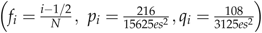
Once more we turn to numerical search, in order to generally characterize the optimal portfolio. Because of computational limits, we only analyze a portfolio of up to N=3 products. We have conducted a search for 75 parameter sets. First, we choose 25 values of e, e=100i (i=1, …, 25), with s=0.0005, S=0.00001. Then, we choose 25 values of s, s=0.00025+0.0001 i (i=1, …, 25), with e=100, S=0.00001. Finally, we choose 25 values of S, S=0.00001+0.000001 i (i=1, …, 25), with s=0.0003, e=100. All search results support three robust observations:
2. Adding the low‐quality layer provides only marginal benefits compared with adding products horizontally. When we add a low‐quality layer, there is a maximum of 11.6% profit increase, based on all parameters sampled. The low‐end products may capture a much larger share of profits and revenues within the portfolio, but compared with having only one product layer, the profit increase is small. In comparison, adding one product horizontally brings in a profit increase of up to 100% (if the market is wide enough to accommodate both products without overlap), which can become less when the market is narrower and forces the products to overlap and horizontally cannibalize each other. When adding a product vertically, market coverage increase happens in the much less lucrative lower segment. When adding products horizontally, the market coverage increase happens in the lucrative upper part of the market. Therefore, adding the low‐quality layer provides only marginal benefits compared with adding products horizontally.
3. When variable costs increase relative to fixed costs, adding a low‐quality product line becomes more attractive. The profit percentage change from one layer to two layers increases with variable cost if we maintain the same fixed cost, and the optimal portfolio should contain only one layer should the variable cost fall below a certain threshold. This is consistent with the result in Section 5 that it is optimal to have only one product line if we have no variable cost.
7.3. Customers Concentrated at the Low End
Section 7.2 assumes that customer preferences are uniformly distributed along both dimensions. This assumption is unrealistic in many social contexts: an important argument for offering low‐end products is the observation that the majority of consumers are characterized by a low‐quality evaluation parameter b (i.e., a low willingness‐to‐pay). In this section, we examine the robustness of the result of the limited value of vertical differentiation, with respect to the distribution of the customer preferences.
Suppose that the distribution of consumers is  . This is a parameterized truncated exponential distribution, where market density decreases with b (more customers at the low end). A higher value of the parameter λ represents a higher concentration of consumers at the low end. As we are not interested in horizontal asymmetries here; we continue to assume that customers are uniformly spread horizontally. We tested the result for the following values of λ: (0.01, 0.02, 0.05, 0.1, 0.2, 0.5, 1, 2, 5, and 10).
We find that for all distributions and starting values, the optimal profit improvement from adding a second (lower quality) product layer does not grow when consumers become more concentrated at the low end (although the market coverage and profit share of the low‐quality product line increase significantly within the portfolio).
When customers are concentrated at the low end, the lower‐quality products account for a higher fraction of demand and profit in the portfolio (up to 50%). However, the profit change from adding the lower‐quality product line remains minimal because of cannibalization. When customers are more concentrated at the low end, the high‐end product layer itself would optimally “shift downward,” lowering its quality and price in order to capture more of the consumers. Therefore, adding lower‐quality products still adds only a small profit, although most of the market is concentrated at the low end. The low value that the low‐end customers place on performance quality turns out to be a fundamental limitation of the profit potential of the low‐end segment, no matter how large this segment is. The literature recommends having vertical differentiated products since consumers are artificially segmented into high end and low end before even designing the product family. However, in our paper, we allow the consumer segments to change, depending on the product offerings. Moorthy (1988) allows for continuous and vertical differentiation, but does not compare profits since he does not have horizontal expansion.
The numerical analyses suggest that the profit potential from adding additional (lower) quality levels in the portfolio is very limited, at 11.6%. Adding horizontal products, in contrast, can multiply profits, provided that the market space is wide enough to “fit them in” without significant cannibalization, even though introducing each horizontal variant incurs a fixed cost. In other words, there is a fundamental difference between the horizontal and vertical market dimensions even when both have enough “room to expand.” The result stems from the very nature of the different preference dimensions of consumers: Horizontally, all customers, and thus the products targeting them, have equal value, because the preferences are not rank ordered. Therefore, profits can be multiplied. Vertically, however, the customers with a low‐quality valuation b are intrinsically less profitable, and so additional quality‐differentiated product lines to target them are less profitable.
8. Conclusions and Discussion
8.1. The Effect of Cost Structure on Product Differentiation
We have considered the positioning of a monopolist's product portfolio in a two‐dimensional market. Customers are vertically heterogeneous in their valuation of performance quality: each individual is characterized by his/her incremental value b for an additional “unit” of quality. Customers are also horizontally heterogeneous in their ideal feature taste: each individual is characterized by an ideal taste parameter a, and they suffer a quadratic utility loss when the product feature deviates from this ideal location. The firm incurs a fixed “design” cost and a volume‐variable “manufacturing” cost, both of which increase quadratically in the quality level. Feature design is cost‐neutral. The firm chooses the number of products and the price, quality level, and feature design for each, in order to maximize profits. The optimal product portfolio exhibits the following properties:
Products with low variable costs relative to design costs (DIPs), such as software or movies, have an optimal portfolio of only horizontal differentiation: all products have the same price and quality levels and are feature differentiated. The entire feature range should be covered for DIPs. Higher variable costs (relative to the fixed costs) favor vertical differentiation. They increase the attractiveness of having multiple quality levels and make vertical differentiation more profitable. Vertical differentiation can be a local optimum only if a low‐quality product covers the entire feature range. In other words, it is optimal to introduce a low‐end product only if it captures sufficient market share. At most, an 11.6% profit increase can be obtained by adding vertical quality levels in the portfolio, even when variable costs are significant and customers are concentrated at the low end of the market. While products of lower quality may account for up to 50% of total revenue, adding such products will increase the profit by a much smaller percentage because of cannibalization: they take share from the profitable high‐end products. This result has an important managerial implication: even though both types of differentiations are limited by fixed design costs, vertical differentiation has only a limited potential to increase profitability. Focusing on the horizontal differentiation has a higher potential if the market has enough room. The low‐quality product line should have more products. There is a maximum of 5.9% increase in profit when we double the number of low‐quality products.
8.2. Discussion: Observations from Practice and Model Limitations
The large size of the low end of the market is a widely used argument to justify low‐end product introduction strategies. Our model suggests that this argument may be a fallacy. Low‐end customers are intrinsically less willing to pay for quality. Therefore, they bring less profit, and attracting them comes at the price of reducing profits. Thus, the sometimes lamented tendency of monopolists to offer only “gold‐plated products” and not recognize lower‐end market potential, may well be the rational profit‐maximizing strategy and not necessarily be due to issues of organizational rigidity or the inability to recognize the low‐end market. Take as an example the “over‐designed” high‐tech telephony offerings of AT&T or Deutsche Telecom until the 1980s, before markets were deregulated. Our model suggests that their high‐end positioning may well have been optimal.
Some industries with low (variable) production costs do indeed exhibit more horizontal differentiation than vertical differentiation, as our model suggests. For example, software products are often differentiated horizontally (with features), but rarely “switch off” features, causing lower functionality in low‐end products (Krishnan and Zhu 2006). iTunes was launched in all European countries with only one quality level for every market. Fashion companies offer numerous horizontal variants, but are reluctant to introduce lower‐quality products under the same brand name in order to avoid cannibalization. Similarly, generic pharmaceutical drugs are often introduced once the patent protection expires, yet under different labels (or even by different companies) to reduce cannibalization. Even during the patent protection era, big pharmaceutical organizations rarely consider blockbuster “versions” of different effectiveness; at the same time, depending on the technological ability, companies try out (horizontally differentiated) drug reception “mechanisms” by the patient.
Once the variable cost for information products turns non‐negligible, vertical differentiation may arise. For example, the iPod and digital camera memory cards have significant production costs, and we observe vertical differentiation. All these industrial practices are consistent with the suggestions of our model.
Yet, vertical differentiation does exist in real markets, even for the cases of DIPs. Does this disqualify our analysis? Like most (if not all) normative research, our modelling effort cannot describe and predict every potential real outcome, as it is constrained by our assumptions. Still, our model adds insights because it suggests that cost structures and customer quality segments do not explain vertical differentiation; there are other mechanisms that may do so. First, Piguovian third‐degree discrimination “assumes that the firm decides what marketing program each segment must receive” (Moorthy 1984: p. 288): the firm can shut down a certain segment's access or exposure to certain products being offered. Second, functionality thresholds may explain vertical differentiation of DIPs. A functionality threshold is a quality requirement that is independent of price; low quality cannot always be compensated by low price (Adner and Levinthal 2001). In such a situation, the low‐quality products do not pose a cannibalization threat to the high‐quality products because they do not satisfy the quality requirement of the high‐end consumers, which is independent of price. Cannibalization, the major reason against vertical differentiation, can be avoided or greatly reduced.
The practice of Microsoft is an example in which functionality thresholds exist. Microsoft offers vertically differentiated products that have different functionalities. High‐end consumers, such as enterprises, cannot use low‐end products regardless of price because they simply do not meet the task requirements. The functionality thresholds change the cannibalization pattern between two products and may make vertical differentiation profitable.
Finally, our model has only one quality dimension. When there are two quality dimensions, which are valued differently by different consumers, two products with different quality levels may co‐exist. However, two such products cannot be really considered vertically differentiated from each other.
Further research is necessary in order to identify other drivers of vertical differentiation, in addition to variable costs as predicted by our model (at least for monopolists). Moreover, we need to examine how the conclusions of our model change under competition. In addition, we have excluded economies of scope in our model. By designing product families, companies can share components and, thus, make the fixed design costs sub‐additive in the number of products.
Footnotes
Acknowledgements
The authors would like to thank the Area Editor, three anonymous referees, Beril Toktay, and Tim van Zandt for helpful comments and suggestions.