
Abstract
Outpatient health care service providers face increasing pressure to improve the quality of their service through effective scheduling of appointments. In this paper, a simulation optimization approach is used to determine optimal rules for a stochastic appointment scheduling problem. This approach allows for the consideration of more variables and factors in modeling this system than in prior studies, providing more flexibility in setting policy under various problem settings and environmental factors. Results show that the dome scheduling rule proposed in prior literature is robust, but practitioners could benefit from considering a flatter, “plateau‐dome.” The plateau–dome scheduling pattern is shown to be robust over many different performance measures and scenarios. Furthermore, because this is the first application of simulation optimization to appointment scheduling, other insights are gleaned that were not possible with prior methodologies.
1. Introduction
Providers of outpatient services are facing increasing pressure to improve the quality of the service they provide. One important dimension is the reduction of waiting times for scheduled appointments. Many researchers have outlined the need to reduce waiting times for outpatients due to increased competition between service providers (Katz et al. 1991), more demanding patients that use waiting time to choose between medical providers (Gopalakrishna and Mummalaneni 1993), the move toward more outpatient services (Goldsmith 1989), and because scheduling policies often favor the service provider (Hamidi‐Noori 1984). In addition, it is desirable to reduce waiting times to minimize contact time between patients. There is a greater chance germs will spread if waiting times are long, the waiting room is full, and/or children are playing in the waiting room. In some cases patients who are anxious about seeing the doctor show more signs of unhealthy stress the longer they wait.
The appointment scheduling problem involves determining an appointment system that includes the start time, duration, and number of appointments for a given session. This is an exceedingly difficult problem, both from a practitioner and research perspective, because of the significant variability in the system (e.g., stochastic arrival and service times, cancellations, and no‐shows). Furthermore, every clinic has its own unique operating and environmental characteristics, and although there have been some notable algorithms developed (e.g. Vanden Bosch et al. 1999, Yang et al. 1998), it is unlikely that a single appointment rule can perform well in all environments (Yang et al. 1998). The wide variation in environmental factors and server tendencies experienced in practice makes this problem too intractable to be solved optimally, even with a single server and the assumption of punctual patients (Robinson and Chen 2003).
The context studied in this research is a static, single server framework where all appointments are made in advance. This is typical of a family physician facility, although the findings can readily be extended to other environments. In particular, this research applies to single‐server, independent queue situations where the service provided is so personal and unique that it usually cannot be done by anyone else. For instance, people generally prefer seeing the same doctor rather than being randomly assigned a physician if there are multiple doctors in a clinic, since a doctor's service is typically more personal (knowledge of patient's medical history makes the service delivery process more efficient). Therefore, the findings here apply best to doctors, specialists, lawyers, and legal aides with full schedules of clients who want and/or need to see a specific individual for the bulk of the service they require.
In this study a simulation optimization algorithm is used where a search heuristic evaluates the output from a simulation model to determine new input values for the simulation to run. The algorithm evaluates uncertainty in the model, and then feeds this information to the heuristic that carries out an intelligent search of the solution space. Therefore, this approach allows for the design of a near‐optimal appointment schedule (AS) while simultaneously evaluating the uncertainty inherent in the system. The main objective of this study is to determine if this algorithm can produce a robust AS given a variety of environmental factors, and thus enhance prior findings from both analytical and simulation studies.
The paper is organized as follows. Section 2 provides a review of the literature on appointment scheduling and solution approaches. Section 3 develops the simulation optimization model. Section 4 presents the scenarios and numerical results. Section 5 concludes with a discussion of the managerial implications for policy design.
2. Literature Review
The appointment scheduling problem can be viewed as one of resource scheduling under uncertainty. While there exist many variants of the problem (e.g., nurse scheduling [e.g., Wright et al. 2006], surgical scheduling [e.g., May et al. 2000, Weiss 1990]), the focus of the discussion here will be on the problem of scheduling N patients in an outpatient facility for a period of time, given uncertainty in the system parameters.
The majority of prior research has involved either the development of optimization algorithms (e.g., Denton and Gupta 2003, Robinson and Chen 2003, Vanden Bosch et al. 1999, Wang 1997, Yang et al. 1998) or used simulation (e.g., Ho and Lau 1992, 1999, Klassen and Rohleder 1996, 2004). Analytical methods have difficulty capturing the complexity of environmental variables and are often restricted to using Erlang or Exponential service times to make the models tractable (Cayirli and Veral 2003). In addition, these methods are often valid for only a small number of patients. Analytical methods used include queuing theory (Brahimi and Worthington 1991, Jansson 1966, Mercer 1960, Pegden and Rosenshine 1990, Stein and Côté 1994), nonlinear programming (Robinson and Chen 2003), stochastic linear programming (Denton and Gupta 2003), and dynamic programming (Fries and Marathe 1981, Liu and Liu 1998). Simulation, on the other hand, while able to evaluate all parameters for a given set of decision variable values, is unable to search for an optimum; the researcher must pre‐determine all possible solutions. The current research attempts to overcome these drawbacks by integrating simulation with metaheuristic framework (OptQuest 2007) that combines scatter search, tabu search, and neural networks to guide a simulation program (Arena; Kelton et al. 2007). Simulation combined with a metaheuristic technique such as scatter search, simulated annealing, or genetic algorithms has been applied in other problem environments (e.g., manufacturing systems design [Azadivar and Tompkins 1999, Pierreval and Tautou 1997, Teleb and Azadivar 1994], single server queuing systems [Fu 2002], inventory control models [Fu 2002, Lopez‐Garcia and Posada‐Bolivar 1999], and environmental policy planning [Huang et al. 2005, Linton et al. 2002]). However, as far as can be determined, this approach has not been applied to an appointment scheduling environment.
Most simulation work has considered either fixed or variable interval appointment systems. Fixed interval appointment systems set the appointment times to some predetermined length (e.g., one appointment every 10 minutes). Variable interval systems allow the length to vary. For instance, Ho and Lau (1992) and Rohleder and Klassen (2000) considered a set of “offset” rules where earlier slots were shorter than average service time, and later slots were longer. In some cases this resulted in extremely late end times for the session. Cayirli et al. (2006) considered this and other variable length appointment rules in conjunction with blocking rules (giving two or more patients the same appointment time). The objective of this study is to determine the best interval appointment system (either fixed or variable) and the best blocking rules to address various research questions.
Another variable interval result found in a few analytical studies is the “dome” pattern, where appointment intervals are initially short, gradually increasing toward the middle of the session, and then decreasing toward the end of the session (Denton and Gupta 2003, Robinson and Chen 2003, Wang 1993, 1997). Wang (1993) finds that the dome rule is optimal for exponential service times while Robinson and Chen (2003) model the problem for the case where the mean of patient service times is allowed to vary, holding the standard deviation of service times constant. Denton and Gupta (2003) develop a two‐stage stochastic optimization model and show that the dome is most pronounced when the doctor's idle time is weighted more heavily than customer waiting times. Each of the above studies used a different performance measure (e.g., Wang [1993] used customer waiting time plus day end time [DET], Robinson and Chen [2003] used customer waiting time plus doctor idle time, and Denton and Gupta [2003] used waiting time, idle time, and overtime). The current study will compare these and other performance measures to determine a set of “base case” scenarios for the analysis.
The dome pattern is an intuitively pleasing result that is able to reduce waiting times as compared with other scheduling rules. One of the challenges with implementation of the dome rule is that each appointment is a slightly different length. While it is straightforward to set up a template for a scheduler to slot patients in, the varying lengths suggest that some appointments will fall at odd times (e.g., 9:05:30 am). Thus, an integer constraint is used in this study to add realism. Furthermore, prior analytical studies have considered seven appointments (Denton and Gupta 2003), 10 appointments (Wang 1993), and up to 16 appointments per session (Robinson and Chen 2003). Empirical work suggests that many doctors schedule six appointments per hour (e.g., Klassen and Rohleder 1996, 2004). Depending on the context and situation, other length appointments are also used. Brahimi and Worthington (1991) report on “plaster‐check” clinics (clinics that check on those who were previously treated at emergency) that schedule 5‐minute appointments, and Cayirli et al. (2006, 2008) reported on general practice clinics in the metro New York area that use 10 appointments of varying length over  . In this study differing numbers of appointments are tested, some scenarios involving many more appointments than have been studied previously. In addition, since this study is not restricted to analytically tractable probability distribution functions, lognormal service times will be used to determine how the dome rule may change under uncertainty (lognormal times have been found empirically (e.g., Cayirli et al. 2006, 2008, Klassen and Rohleder 1996, O'Keefe 1985).
3. Model Development
Simulation optimization is a stochastic optimization method that enables a search for solutions in problems where some or all of the system parameters are stochastic (Fu 2002, Law and Kelton 2000). It is well suited for problems where uncertain parameters can be represented by probability distribution functions. The problem formulation for simulation optimization algorithms specifies the objective function and constraints as a set of discrete‐event simulation models in which a heuristic guides the search for an optimum. This method can significantly decrease the time and cost of solving such a system since it limits the number of simulations that are needed to find an (near) optimal configuration for the system (i.e., there is no need to exhaustively consider all possible configurations as when simulation is used alone).
3.1. The Algorithm
Heuristic approaches are useful for addressing problems for which no analytical solution method exists but where analytical formulations of the objective function and constraints do exist. In combining simulation with a heuristic, the problem is approached by iteratively generating sets of decision variable values that are evaluated by simulation. In this study, the solution search is directed by several metaheuristic procedures, with the primary heuristic being scatter search. The metaheuristic also includes secondary heuristics based on tabu search, integer programming, and neural networks (OptQuest 2007). A general formulation of the problem can be written as 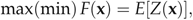

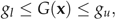

Scatter search is an evolutionary method that has shown great potential for solving difficult combinatorial and nonlinear optimization problems (Glover 1994, Marti et al. 2006). Furthermore, this heuristic is well suited for appointment scheduling problems with integer decision variables because scatter search was originally developed to address problems containing integer decision variables. A distinguishing feature of scatter search heuristics is a mapping mechanism used to translate points that are not feasible into a feasible point rather than removing it from consideration. Furthermore, since the search mechanism is population based, it permits the algorithm to simultaneously search many areas of the search domain. Tabu search is used both to ensure diversity in the population and to prevent the algorithm from revisiting solutions that have proven to be sub‐optimal. A brief summary of how the simulation module interacts with the scatter search/tabu search optimization procedure for the appointment scheduling application is given in Figure 1.
3.2. Simulation Model
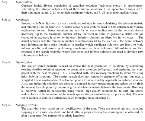
The simulation module is similar to prior studies. Most doctors schedule session lengths between 3 and 4 h and, thus, the session length for this study is set at  . To initialize the algorithm, minimum start times for all appointments are set to zero, maximum times to 210 minutes, and median times to 105 minutes. The lognormal distribution is used for service times (which has been found empirically (e.g., Cayirli et al. 2006, 2008, Klassen and Rohleder 1996, O'Keefe 1985). It has been shown that the lower the coefficient of variation (CV), the better the performance of the AS (Ho and Lau 1992, Klassen and Rohleder 1996), and that this effect is consistent across different AS (Klassen and Rohleder 2004). Thus, different CV values are not tested here. However, it is likely that different patients in the same system have different variances. As such, a continuous‐variance lognormal distribution is used (as in Rohleder and Klassen 2000). If s
i
denotes the time it takes to serve patient i, then s
i
is distributed as follows:
. To initialize the algorithm, minimum start times for all appointments are set to zero, maximum times to 210 minutes, and median times to 105 minutes. The lognormal distribution is used for service times (which has been found empirically (e.g., Cayirli et al. 2006, 2008, Klassen and Rohleder 1996, O'Keefe 1985). It has been shown that the lower the coefficient of variation (CV), the better the performance of the AS (Ho and Lau 1992, Klassen and Rohleder 1996), and that this effect is consistent across different AS (Klassen and Rohleder 2004). Thus, different CV values are not tested here. However, it is likely that different patients in the same system have different variances. As such, a continuous‐variance lognormal distribution is used (as in Rohleder and Klassen 2000). If s
i
denotes the time it takes to serve patient i, then s
i
is distributed as follows: 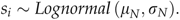
The mean (μ
N
) is the length of the session divided by the number of appointments scheduled per session, N. The standard deviation is defined as 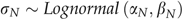 . For example, the values used for N=21 are as follows: μ
N
=10 minutes, α
N
=7.5, and, β
N
=7.5. For each scenario the simulation module is allowed to run as many replications as required to obtain a stable solution.
. For example, the values used for N=21 are as follows: μ
N
=10 minutes, α
N
=7.5, and, β
N
=7.5. For each scenario the simulation module is allowed to run as many replications as required to obtain a stable solution.
3.3. Performance Measures
There are many options when choosing performance measures (Cayirli and Veral 2003). It is desirable to test a wide range of performance measures for two main reasons. First, this is an initial study using simulation optimization. Given the probabilistic nature of the search process, testing various measures and comparing results to prior studies helps establish that the algorithm is converging on optimal regions of the solution space. Second, there is value in understanding how results differ for different measures. The performance measures used include the total cost of patients' waiting time and doctor's idle time, overtime, and DET. Table 1 provides the measures studied in this paper and examples of prior studies where they have been used. The following notations are used:
DET is not equivalent to OT, since if DET is less than the regular session end, then OT is zero (i.e., OT cannot be negative).
** WIT and DET not formulated as a composite measure by Klassen & Rohleder, but are used together to compare scenarios.
N=number of appointments scheduled per session x
i
=appointment time of patient i, i=1, 2, 3, … N
CWT
i
=waiting time for patient i
IT
i
=physician idle time between appointment i and i−1 DET=day (session) end time for physician OT=overtime for physician per session s
i
=service time for patient i (Equation [5]) c
w
=cost coefficient for patient waiting c
o
=cost coefficient for physician overtime c
it
=cost coefficient for physician idle time d=length of session (in this study d usually=210 minutes)
3.4. Problem Formulation
The algorithm was set up to minimize each of the performance measures subject to different constraints depending on the research question being addressed. It is assumed that patients and the doctor arrive punctually (neither late nor early), that is, x
1=0, CWT
1=0, and IT
1=0. It follows that 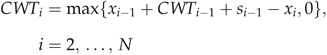
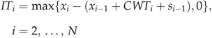


A general formulation for the performance measures used in the study is given by 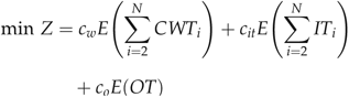


Note that successive appointments could be scheduled to start at the same time. Thus, this formulation tests, among other things, whether double‐booking or “block” AS are a good solution. Also, it is not necessary to constrain x i ≤d if the cost structure is used to control overtime, as occurs in a number of scenarios tested. However, it is interesting to consider a few cost structures that tend to spread appointments out, causing excessive overtime. In order to locate a schedule that avoids this unrealistic outcome, this constraint is required. In these cases boundary solutions are obtained.
3.5. Validation of the Approach
Given the stochastic nature of this system, there are many possible solution configurations that exist. Consequently, the quality of the solutions generated can be highly variable (Andradóttir 2002). Although scatter search is able to offset this effect by performing an intelligent and extensive search of the solution space, the search mechanism is a probabilistic one and therefore different experiments will lead to different solutions.
In order to validate the robustness of the proposed procedure, its performance was tested against the “optimal” algorithmic solutions generated by Vanden Bosch et al. (1999), Yang et al. (1998), and Robinson and Chen (2003). These analytical studies involve similar problem environments to the current study, which make them suitable for testing the simulation optimization methodology. The problem formulations and performance measures used in these studies were set up as simulation optimization models. The goal was to determine if the simulation optimization algorithm is capable of finding near‐optimal solutions for these problem formulations. The simulation optimization approach used in this study was able to find solutions that were 6.1%, 2.5%, and 0.5% better, respectively, for the mean of the performance measure. This does not suggest that the simulation optimization algorithm is superior since the problem test bed contains stochastic elements that were not designed to be addressed by these analytical studies. However, the results demonstrate that the procedure is adept at identifying good solutions. In the case of the dome rule, the percentage change in results is extremely small. This is unsurprising since the dome has been shown to be superior in prior analytical studies (Denton and Gupta 2003, Robinson and Chen 2003, Wang 1993).
The algorithm was also compared with rules found in prior simulation studies. Results from a simulation optimization run for a similar environment to those used in prior studies are compared with five rules that have been identified as superior using WIT as the performance measure. The first three are based on Cayirli et al. (2008), who found three basic patterns that performed well under different environmental circumstances. These were (i) scheduling patients in individual blocks at fixed intervals (IBF); (ii) a “multiple block, fixed interval” rule where two patients are scheduled at the same time (MBFI); and (iii) placing two appointments in slot 1, the third patient in slot 2, and so on (2BEG). Another rule that performs well for the doctor is placing four patients in the first slot, the fifth patient in the second slot, and so on (“4BEG”; Bailey 1954). A fifth rule was identified by Rohleder and Klassen (2000) when they adjusted the parameters in an Offset rule (discussed above) to improve results. Table 2 demonstrates that simulation optimization is able to find superior solutions for WIT when compared with these rules.


Based on WIT performance measure and no constraint on session end time.
See Table 1 for explanations for abbreviations.
4. Results and Analysis
In this study several different clinic scenarios are examined. The best AS are determined under various combinations of factors including number of appointment slots, probability of no‐shows, and DET and cost structures including cost of doctor idle time and overtime. The experimental design is aimed at addressing two major issues. The first issue pertains to the simulation optimization algorithm's ability to generate optimal solutions in an appointment scheduling environment. The second issue relates to finding solutions/schedules that may provide insights for policy makers.
Initially, the performance measures in Table 1 are tested in order to establish a set of “base case” scenarios for subsequent experiments and compare results for different measures. Subsequently, experiments with N identical patients and five values for N (N=7, 10, 14, 21, 42) are considered, which correspond to five appointment lengths, ranging from 5 to 30 minutes. The performance measure reflects various weights for patient waiting vs. server idle time, testing three cost coefficients for server idle time (c it =1, 5, 10) for each value of N, representing 15 clinic scenarios.
It is also worthwhile to investigate the performance of the algorithm in determining AS for more complex clinic environments. First, four levels of no‐shows (0%, 10%, 20%, 30%) are tested. Second, the model is run for two different length sessions ( and
and  h). Finally, DET is used to constrain the length of the session at four levels (210, 220, 230, 240 minutes).
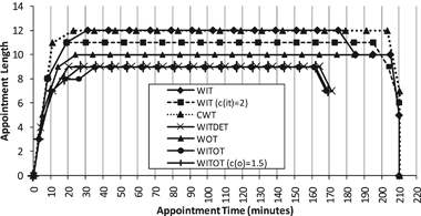
4.1. Comparison of Performance Measures
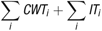
Given the probabilistic nature of simulation optimization, it is helpful to establish a basis of comparison for subsequent experiments. Thus, the five performance measures in Table 1 were tested, with results shown in Table 3. Results for each component of the objective function are presented in times (rather than costs) in order to reflect how the performance measures affect the patients and doctor. Modifications of two of the measures have been used in a number of studies, and results for these are also tested. The measures are WIT with c it =2 (e.g., Robinson and Chen 2003, Yang et al. 1998) and WITOT with c o =1.5 (e.g., Cayirli et al. 2006, Denton and Gupta 2003, Liu and Liu 1998).


*Maximum appointment time=210 min; no constraint on session end time.
See Table 1 for explanations for abbreviations.
In order to better show the tradeoff between patient waiting and server idle time, it is helpful to plot these rules on an efficient frontier, as is done in Figure 2. All rules are on the frontier except WITOT (c o =1.5).
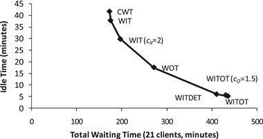
Table 3 and Figure 2 show that the schedules generated vary significantly, depending on the performance measure used. This is discussed further in Section 4.3 after some further analysis is completed.
Although appointment times are constrained to be integers, it can be argued that the times found by the algorithm would be difficult to implement because they do not occur at 5‐minute intervals; it may be difficult for patients to show up at “odd” times (such as 9:12 or 9:29). In prior studies this practicality has often been ignored (e.g., most analytical studies, any of the Offset or Dome rule formulations), but of interest is whether rounding each appointment to the nearest 5‐minute interval will seriously degrade the performance measures. This was carried out for the above scenarios, with positive results. For instance, running this with the WIT measure produces a 2.1% increase in WIT and a 3.2% increase in CWT, while IT is actually 7.1% better, and DET is 1.2% better. This suggests that rounding appointment times to the nearest 5‐minute interval may have little effect on the performance of the system.
4.2. Variation in Number of Appointments and Cost Structure
Some doctors may require different length appointments, depending on their specialty area. At the same time, it is often true that the doctor's time is more valuable than the patients' time. To explore these questions, experiments were run for the problem defined in (10)–(13) for N=7, 10, 14, 21, and 42, c
it
=1, 5 and 10, c
w
=1, and c
o
=0. The  ‐hour session length was maintained, meaning that different scenarios had appointments of varying length (e.g., 10 minutes for N=21). The standard deviation of appointment times is as specified in Section 3.2.
The schedules generated for the N=21 case are shown in Figure 3. The vertical gridlines represent the time of each appointment if fixed‐interval, 10‐minute appointments were scheduled. The AS across all scenarios tested had very different performance measure values but followed a similar pattern. The costs of the system are similar to the results found by Denton and Gupta (2003) and are approximately linearly increasing in the number of patients scheduled.
4.3. Pattern of Appointments
One of the goals of this study is to determine if the simulation optimization approach is able to identify new scheduling patterns. The schedules in Figure 3 show that the best AS have appointments spread fairly uniformly across most of the scheduling session. The major deviations to this occur at the beginning and end of the session, where slots are often shorter. This pattern is consistent across all 15 of the scenarios tested and, thus, partially supports prior findings that a dome pattern maximizes performance (Denton and Gupta 2003, Robinson and Chen 2003, Wang 1993, 1997). However, the dome shape is not as pronounced as was found previously; a small number of slots at the beginning and end are shorter while the intermediate appointments are approximately the same length. This is consistent with the pattern found by Robinson and Chen (2003), but is extended here to include larger values for N. We refer to this pattern as a “plateau–dome.”
From the standpoint of practical implementation of the plateau–dome scheduling rule, it is worthwhile to consider an appointment rule whereby all slots that correspond to the plateau portion of the dome are constrained to be of equal length. This was achieved by running each scenario a second time with the added constraint: 
The support values α and β are the appointment slots corresponding to the beginning and end of the plateau portion, respectively, which were determined from the initial run for that scenario. Results from this second run are shown in Appendix A. Performance is only slightly reduced with the addition of the constraint; on average, 0.22% worse over all 15 scenarios. This suggests that the plateau–dome may be robust over a wide range of operational settings. It is also evident that a higher cost coefficient for the doctor's time is associated with lower levels for the plateau. This bunches patients together throughout the session, causing them to arrive earlier, loading the system and reducing idle time.
An interesting result occurs for N=42 and c it =10. The plateau settles on 5‐minute slots then improves by adding three 6‐minute appointments in the middle (δ 17−δ 19). (This was obtained by relaxing [14] and running the scenario a third time with the plateau result as a starting point). This pattern more closely resembles a dome pattern, although the dome is “limited” because the algorithm did not find more than two different values for the intermediate appointments intervals. This highlights the difficulties imposed by the integer constraint, which may make it challenging to determine at what level the plateau should be. This suggests that in some cases policy makers can have more flexibility in setting schedules by considering a “two‐tier plateau.”
The patterns generated for the initial scenarios reported in Table 3 exhibited similar plateau‐like characteristics and were also run with constraint (14) in order to determine the performance of the plateau–dome scheduling rule. Performance is, on average, only 0.66% worse than in Table 3, with the maximum being 1.19% worse.
Figures 2 and 4, and Table 3 together demonstrate that the plateau length relative to session length and the position of the plateau are informative in identifying measures that favor the server or the client. In general, client‐oriented measures such as CWT and WIT produce AS where the plateau is higher and longer, with more appointments bunched at the end of the session. Server‐oriented measures such as WITDET, WITOT, and WITOT (c o =1.5) result in AS where the plateau is lower and shorter and clients are bunched at the beginning of the session. This suggests the plateau–dome may be robust over many different clinic environments.
4.4. Incorporating No‐Shows
Cayirli and Veral (2003) showed that the presence of no‐shows has a large effect on a scheduling system. In order to test the robustness of the plateau–dome pattern under a variety of conditions, the effects of no‐shows are considered. For the problem defined in (10)–(13) experiments were run with the probability of no‐shows at four levels (0%, 10%, 20%, 30%) representing typical levels found in practice. Based on initial experiments, four performance measures were chosen that provide a wide range of client‐oriented and server‐oriented measures (WIT, WOT, WITDET, and WITOT [c o =1.5]) to test their impact on the performance of the AS. Representative results for two measures (WIT and WOT) are shown in Table 4.


All values compared with those in Table 3 for WIT and WOT.
See Table 1 for explanations for abbreviations.
Results show that the best AS follow an approximate plateau–dome for these scenarios, and thus, all were re‐run with constraint (14). This resulted in only an average 0.19% drop in performance. In general, the higher the level of no‐shows, the lower the plateau. As the percentage of no‐shows increases, idle time increases and waiting time, DET, OT, and the time of the last appointment all decrease. The improvement in performance measures is attributable to the reduced workload for the doctor. This suggests clinics may compensate based on the expected probability of no‐shows by overbooking patients (Blanco White and Pike 1964, Vissers 1979) or reducing the length of the appointment slots (Vissers 1979, Vissers and Wijngaard 1979).
The results also suggest a double‐booking strategy. For measures that favor the doctor, the best AS often have the first two patients placed at time zero (i.e., double‐booked) with the rest of the patients spread out evenly across the plateau. Furthermore, as the level of no‐shows increases, the third patient tends to also be scheduled early (1–4 minutes). This supports the findings of Jansson (1966) who suggests booking two patients in the first slot when there are no‐shows. The pattern found here only blocks the first two patients; this is in contrast to the findings of Cayirli et al. (2006), who find that blocking patients throughout the session improves performance—although they suggest that this may be due to the presence of patient unpunctuality in their model.
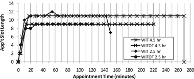
4.5. Different Length Sessions and End‐of‐Day Restrictions
Experiments were also run for  and
and  ‐hour sessions using 10‐minute appointments (N=15 and 27, respectively) for the problem defined in (10)–(13) to test the sensitivity of the plateau–dome pattern to changes in session length. This was done for one client‐oriented measure (WIT) and one server‐oriented measure (WITOT). All four scenarios resulted in plateau‐like patterns, and were subsequently run with constraint (14). The results from one scenario (WIT
  hour) suggested that a third run was warranted (for the same reasons listed above in Section 4.3), and this resulted in a short second tier. Overall, performance was only 0.83% worse with this constraint (Figure 5).
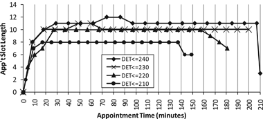
Another question of interest is what AS would be required to “guarantee” a time that the doctor will be finished with patients, or in terms of the measures used here, to guarantee a particular DET or a maximum level of overtime. Some doctors allow time at the end of their day where patients are not scheduled, which they may use to finish serving patients or to book urgent patients (Klassen and Rohleder 2004), but of interest here is when the doctor should expect to be finished with scheduled patients. Prior studies have, for the most part, ignored this constraint. Some have had overtime in their objective function, but few, if any, have imposed a constraint on the maximum level of overtime or when the doctor is finished for the session. Table 5 shows results for DET constrained to four levels (210, 220, 230, 240 minutes), using WIT as the performance measure.


All values compared to those in Table 3 for WIT.
See Table 1 for explanations for abbreviations.
A restriction of 210 minutes results in the last appointment scheduled at time 154 (56 minutes before the end of the session) and excessive waiting for patients. Thus, although it may be attractive for a doctor to know when they will be finished serving patients, the cost in terms of patient waiting is very high. The patterns for these again follow the plateau–dome (Figure 6), with two having a short second tier (DET≤240 and DET≤230). In this case constraint (14) resulted in a 0.63% increase in the performance measures.
5. Discussion and Conclusions
This study suggests a new methodological approach, simulation optimization, for the appointment scheduling problem. As with any simulation optimization research, the integration of analytical and simulation methods is explored, in turn strengthening the “bridge” between theoretical and practical perspectives. The major findings are:
Simulation optimization is effective at identifying good AS when compared with results found in prior analytical and simulation studies. This approach is able to locate high‐quality solutions while simultaneously capturing uncertainties (e.g., service times, no‐show rates) in the system. The method is flexible in finding solutions for a wide variety of performance measures, variables, and number of appointments. The results support a modification, for practical implementation, of the prior‐suggested dome pattern (Denton and Gupta 2003, Robinson and Chen 2003, Wang 1993, 1997). The modification involves a flattened dome that we denote a “plateau–dome.” The plateau–dome pattern is robust across different performance measures, number of appointments, appointment lengths, cost factors, levels of no‐shows, session lengths, and DET restrictions. The pattern is adjusted depending on the environment. For instance, as the value of the doctor's time increases, the plateau becomes lower and shorter relative to session length. Similarly, higher, longer plateaus favor the client, spreading appointments out and reducing waiting time. In a few cases a “second tier” on the plateau can improve performance of the AS. This occurs when the best plateau height is between two integer levels and the algorithm is not able to adjust the length of the plateau to compensate. The presence of no‐shows introduces the strategy of double‐booking. This study suggests that, if compensating measures such as overbooking are not used, the best solution is to book the first two clients at the beginning of the session (time zero) and, as no‐shows levels become higher, to shorten the appointment slots on the plateau. A restrictive session end time results in excessive client waiting, suggesting that a guaranteed end of session time for the doctor can significantly reduce the performance of the AS.
Future research can build on these results by exploring whether the plateau–dome pattern is robust for more complex environments including disruptions to the system, doctor and patient unpunctuality, and heterogeneous clients.
Footnotes
Appendices
Acknowledgments
This research was supported by Canada's Natural Sciences and Engineering Research Council (NSERC), Discovery Grant #283333.